Probing Higgs-portal dark matter with vector-boson fusion

Abstract

We constrain the Higgs-portal model employing the vector-boson fusion channel at the LHC. In particular, we include the phenomenologically interesting parameter region near the Higgs resonance, where the Higgs-boson mass is close to the threshold for dark-matter production and a running-width prescription has to be employed for the Higgs-boson propagator. Limits for the Higgs-portal coupling as a function of the dark-matter mass are derived from the CMS search for invisible Higgs-boson decays in vector-boson fusion at $13\text{\,}\TeV$. Furthermore, we perform projections for the $14\text{\,}\TeV$ HL-LHC and the $27\text{\,}\TeV$ HE-LHC taking into account a realistic estimate of the systematic uncertainties. The respective upper limits on the invisible branching ratio of the Higgs boson reach a level of $2\text{\,}\mathrm{\char 37\relax}$ and constrain perturbative Higgs-portal couplings up to dark-matter masses of about $110\text{\,}\GeV$.

1 Introduction

The existence of dark matter (DM) constitutes one of the main puzzles in modern physics. It has stimulated a broad range of experimental tests, ranging from direct and indirect detection experiments to searches for DM candidates at the LHC Bertone:2010zza .

Minimal Higgs-portal models are particularly simple, supplementing the Standard Model (SM) by the DM field only Silveira:1985rk ; McDonald:1993ex ; Burgess:2000yq . The interaction of DM with the SM is mediated by the SM Higgs boson alone. We concentrate on the case of scalar DM, which has the compelling feature that the portal interaction is renormalizable. For higher-spin choices of the DM field, the model can be considered as an effective description, necessitating the introduction of further fields to restore renormalizability and unitarity at high energies Kim:2008pp ; LopezHonorez:2012kv ; Baek:2012se ; Walker:2013hka ; Freitas:2015hsa .

The model is phenomenologically attractive if the DM mass satisfies $m_{\text{DM}}\sim m_{h}/2$ such that DM annihilation is resonantly enhanced. This region of parameter space is of particular interest as it reconciles the relic density constraint and the strong limits from direct detection. As a matter of fact, the resonance region constitutes one of the two preferred regions in global fits of the model (see e.g. Athron:2017kgt ; Athron:2018ipf ), taking into account constraints from the relic density, invisible Higgs decays, direct and indirect detection. While current limits from direct detection Aprile:2018dbl exclude the region above the resonance up to $m_{\text{DM}}\sim$1\text{\,}\mathrm{TeV}$$, indirect detection potentially imposes relevant constraints only in a narrow window Feng:2014vea , as the velocity-averaged annihilation rate today peaks sharply around $m_{\text{DM}}=m_{h}/2\,\pm\,\mathcal{O}(\Gamma_{\text{tot}})$, where $\Gamma_{\text{tot}}$ is the total Higgs width. However, parts of this region turn out to be preferred when fitting an indirect detection signal within the model, such as the gamma-ray Galactic center excess or the cosmic-ray antiproton excess Cuoco:2016jqt ; Cuoco:2017rxb . In this case the fit is sensitive to changes of the DM mass of the order of $\Gamma_{\text{tot}}$.

While LHC searches are not sensitive to couplings that lead to the measured relic density in a canonical freeze-out scenario for $m_{\text{DM}}\gtrsim m_{h}/2$, larger couplings might be realized in nature, when deviating from the standard scenario. For instance, the scalar particle may not make up all of DM. This case could even be preferred for DM masses around the resonance as discussed in Cuoco:2016jqt ; Cuoco:2017rxb . In alternative models, the scalar particle is not itself the DM candidate but a co-annihilating partner within a dark sector. In this case the region of very efficient annihilation (that would lead to highly under-abundant DM in the canonical scenario) is of particular interest. It opens up the possibility of achieving the measured relic density for example via conversion-driven freeze-out Garny:2017rxs ; DAgnolo:2017dbv . In this case the metastable singlet scalar would escape the detector invisibly. A similar scenario has been considered in Maity:2019hre . Deviating even further from canonical assumptions, the coupling required by the relic density constraint can be largely altered by a non-standard cosmological history Kamionkowski:1990ni , while direct detection limits can be relaxed in minimal extensions of the singlet scalar Higgs portal model Gross:2017dan ; Casas:2017jjg ; Bhattacharya:2017fid . This potentially reopens the parameter space above the resonance and renders collider experiments to be a unique probe of the model.

In this work, we derive limits on the Higgs-portal coupling from an LHC search in the vector-boson fusion (VBF) channel Jones:1979bq ; Cahn:1983ip which is a particularly promising channel to search for DM with couplings to the SM Higgs boson only Eboli:2000ze . Several Higgs production channels have been investigated in the past Craig:2014lda ; Endo:2014cca ; Han:2016gyy ; Dercks:2018wch ; Arcadi:2019lka and it has been shown that the VBF channel is the most sensitive one, motivating extensive studies of this channel in searches for invisible Higgs decays and Higgs-portal DM at current and future colliders Bernaciak:2014pna ; Goncalves:2017gzy ; Biekotter:2017gyu ; Buttazzo:2018qqp ; Sirunyan:2018owy ; Aaboud:2018sfi ; Ruhdorfer:2019utl .

As we have argued before, the Higgs resonance is of particular interest. However, LHC studies have either considered the on-shell regime, constrained by the invisible Higgs branching ratio (see e.g. Ref. Sirunyan:2018owy ; Aaboud:2018sfi for recent experimental results), or heavier DM particles which are produced via a highly off-shell Higgs boson Craig:2014lda ; Endo:2014cca ; Ruhdorfer:2019utl . In this paper we close this gap by calculating limits on the Higgs-portal model with a special emphasis on analysing the region with $m_{\text{DM}}\sim m_{h}/2$. For $m_{\text{DM}}=m_{h}/2\pm\mathcal{O}(\Gamma_{\text{tot}})$ and sizeable DM couplings, the total Higgs width as a function of the invariant mass varies substantially and distorts the Higgs-boson line-shape due to the opening of the Higgs decay into DM. As a consequence, a fixed-width computation becomes unreliable and needs to be improved using a running width in the Higgs propagator.

We reinterpret the $13\text{\,}\mathrm{TeV}$ VBF analysis for invisble Higgs-boson decays by CMS Sirunyan:2018owy to establish limits on the Higgs-portal coupling as a function of the DM mass. In particular, we utilize the bounds on the signal strength for the production of an additional invisibly-decaying SM-like Higgs-boson $\cal H$ with mass $m_{\cal H}$ that does not mix with the SM Higgs boson to compute the limits. In addition to the reinterpretation of the $13\text{\,}\mathrm{TeV}$ analysis of Ref. Sirunyan:2018owy , we derive prospects for the $14\text{\,}\mathrm{TeV}$ HL-LHC on the basis of Ref. CMS:2018tip , and for a possible $27\text{\,}\mathrm{TeV}$ HE-LHC upgrade. In contrast to considering ultimate sensitivities Craig:2014lda ; Endo:2014cca ; Ruhdorfer:2019utl , we put particular emphasis on estimating the systematic uncertainties on the data-driven background prediction. As a by-product of our analysis within the singlet scalar Higgs-portal model, in analogy to Ref. Sirunyan:2018owy , we derive projected limits on the on-shell production of an additional Higgs-boson $\cal H$. These results might be useful to constrain other models using the procedure outlined in this work.

The remainder of this paper is organized as follows. In Sec. 2 we briefly introduce the singlet scalar model. In Sec. 3 we derive current $13\text{\,}\mathrm{TeV}$ constraints. Projections for the HL- and HE-LHC are studied in Sec. 4. We conclude in Sec. 5. Appendix A provides more details on the running-width prescription and Appendix B discusses alternative choices regarding the spin of the DM candidate.

2 Higgs portal model

We consider the scalar singlet Higgs-portal model Silveira:1985rk ; McDonald:1993ex ; Burgess:2000yq , which is among the simplest possible UV-complete extensions of the SM. It extends the SM by a real singlet scalar field $S$ that is stabilized by a $Z_{2}$ symmetry and thereby provides a DM candidate. The corresponding Lagrangian is

$$\mathcal{L}=\mathcal{L}_{\text{SM}}+\frac{1}{2}\partial_{\mu}S\,\partial^{\mu}S-\frac{1}{2}m_{S,0}^{2}S^{2}-\frac{1}{4}\lambda_{S}^{2}S^{4}-\frac{1}{2}\lambda_{\text{HP}}S^{2}\,\Phi^{\dagger}\Phi\,,$$ (1)

where $\Phi$ is the SM Higgs doublet. After electroweak symmetry breaking, in unitary gauge we can write $\Phi=(0,h+v)/\sqrt{2}$, where $v\simeq$246\text{\,}\mathrm{GeV}$$ is the SM Higgs vacuum expectation value and the scalar mass is given by $m_{S}^{2}=m_{S,0}^{2}+\lambda_{\text{HP}}v^{2}/2$. The Higgs-portal coupling induces the interactions

$${\cal L}_{\text{HP}}=-\frac{1}{4}\lambda_{\text{HP}}\,h^{2}S^{2}-\frac{1}{2}\lambda_{\text{HP}}v\,h\,S^{2}\,,$$ (2)

where the latter is relevant for the phenomenology considered here.

If $m_{S}<m_{h}/2$, the Higgs boson can decay invisibly into two DM scalars with the decay width

$$\Gamma_{\text{inv}}=\frac{\lambda_{\text{HP}}^{2}v^{2}}{32\pi m_{h}}\sqrt{1-4\frac{m_{S}^{2}}{m_{h}^{2}}}\,.$$ (3)

For an extensive discussion of the DM and collider phenomenology of this and other Higgs-portal models, we refer the reader to the recent and comprehensive review Ref. Arcadi:2019lka and references therein.

3 LHC limits at 13 TeV

In this section, we derive limits on the Higgs-portal coupling $\lambda_{\text{HP}}$ in Eq. (1) using the results of the $13\text{\,}\mathrm{TeV}$ CMS search for invisible Higgs decays in the VBF channel as reported in Ref. Sirunyan:2018owy . The corresponding ATLAS study can be found in Ref. Aaboud:2018sfi . In VBF, the Higgs boson is produced in association with two jets (see Figure 1) that are characterised by a large separation in pseudorapidity and by a large dijet invariant mass. The search presented in Ref. Sirunyan:2018owy is based on a cut-and-count and on a shape analysis, where the shape of the dijet invariant mass is used to impose limits on the invisible branching ratio of the SM Higgs boson. In addition, limits on the production cross section for a SM-like heavy Higgs boson are reported, assuming a branching ratio of one for the decay into invisible final states and no mixing with the SM Higgs.

Figure 1: Feynman diagram for Higgs-portal DM production in VBF at the LHC.

In Section 3.1, we derive limits on the Higgs-portal coupling $\lambda_{\text{HP}}$ exploiting all the results of Ref. Sirunyan:2018owy . In particular, we show how the cross-section limits on an additional heavy Higgs boson can be used to derive limits on $\lambda_{\text{HP}}$ for DM masses in the vicinity and beyond the threshold, where the on-shell Higgs decay into DM particles is kinematically inaccessible. We employ both the cut-and-count analysis as well as the shape analysis.

In Section 3.2, we recast the cut-and-count analysis of Sirunyan:2018owy using leading-order (LO) Monte Carlo simulations. Employing a simple rescaling of the LO cross sections to match the more sophisticated predictions in Ref. Sirunyan:2018owy , we reproduce the bounds on the Higgs-portal coupling as found in Section 3.1. This validation of our Monte Carlo setup enables us to perform projections for searches at the $14\text{\,}\mathrm{TeV}$ high-luminosity LHC as well as at a $27\text{\,}\mathrm{TeV}$ high-energy LHC option in Section 4.

3.1 Reinterpretation of upper limits

In the following, we assume a factorization of Higgs production and decay, i.e. we do not consider electroweak corrections or higher-order corrections in the Higgs-portal coupling. In this approximation, one can write any fiducial cross section $\sigma_{\text{inv}}$ for the production of a pair of DM particles (or any other pair of invisible particles coupling exclusively to the Higgs boson) as

$$\sigma_{\text{inv}}=\int\frac{\mathrm{d}q^{2}}{2\pi}\,\sigma_{h}(q^{2})\,|P(q^{2})|^{2}\,2q\,\Gamma_{\text{inv}}(q^{2})\,\Theta(q^{2}-4m_{S}^{2})\,,$$ (4)

where $\sigma_{h}(q^{2})$ is the corresponding fiducial, detector-level production cross-section (including acceptance times efficiency) of the (off-shell) SM Higgs boson at a given invariant mass $q^{2}$. The Higgs-boson propagator is denoted by $P(q^{2})$ and the partial Higgs-boson width $\Gamma_{\text{inv}}(q^{2})$ generalizes the result of Eq. (3) by replacing the Higgs mass $m_{h}$ with $\sqrt{q^{2}}$. Well below threshold ($m_{S}<m_{h}/2$), the on-shell Higgs-boson decay into invisible DM particles is open. Hence, as long as the Higgs-portal coupling is not too large, the narrow-width approximation applies and the right-hand-side of Eq. (4) reduces to the product of the on-shell Higgs-production cross-section and the branching ratio into DM pairs. For this case, Ref. Sirunyan:2018owy has already interpreted its bound on the invisible branching ratio of the Higgs boson in terms of the Higgs-portal model (see Figure 10 of Ref. Sirunyan:2018owy ).

In this work, we also address DM masses in the threshold region and beyond, where DM production involves an off-shell Higgs boson. In this context, in order to obtain $\sigma_{h}(q^{2})$ from the experimental analysis, we employ the interpretation of the VBF+MET search in terms of an additional SM-like Higgs boson $\cal H$ that does not mix with the $125\text{\,}\mathrm{GeV}$ Higgs boson and decays to invisible particles. This interpretation provides a limit $\mu_{\mathcal{H}}^{95\%}$ at the $95\text{\,}\mathrm{\char 37\relax}$ confidence level (CL) on the signal strength $\mu_{\mathcal{H}}=\sigma\times{\cal B}({\cal H}\to\text{inv})/\sigma_{\text{SM}}$ as a function of the mass $m_{\cal H}$ of the additional Higgs boson for the cut-and-count as well as the shape analysis (see Figure 7 in Ref. Sirunyan:2018owy ). Hence, any BSM contribution $\sigma_{\text{inv}}$ to the cut-and-count measurement has to be smaller than the corresponding limit

$$\sigma_{\text{inv}}^{95\%}=\mu_{\mathcal{H}}^{95\%}(m_{\mathcal{H}})\sigma_{\text{SM}}(m_{\mathcal{H}})=\mu_{\mathcal{H}}^{95\%}(q^{2})\sigma_{h}(q^{2})\,,$$ (5)

where we have used $\sigma_{h}(q^{2}=m^{2}_{\mathcal{H}})=\sigma_{\text{SM}}(m_{\mathcal{H}})$, i.e. the on-shell production cross section for an additional SM-like Higgs boson is identical to the off-shell SM Higgs-boson cross section at $q^{2}=m^{2}_{\mathcal{H}}$, if electroweak corrections are ignored. Note that $\sigma_{\text{inv}}^{95\%}$ is, of course, independent of $m_{\mathcal{H}}$ or $q^{2}$. Using Eq. (5) to eliminate $\sigma_{h}(q^{2})$ in Eq. (4), and dividing by $\sigma_{\text{inv}}^{95\%}$, one finds

$$\frac{\sigma_{\text{inv}}}{\sigma_{\text{inv}}^{95\%}}=\int\frac{\mathrm{d}q^{2}}{2\pi}\,\frac{1}{\mu^{95\%}_{\mathcal{H}}(q^{2})}\,|P(q^{2})|^{2}\,2q\,\Gamma_{\text{inv}}(q^{2})\,\Theta(q^{2}-4m_{S}^{2})\,.$$ (6)

Since only $\sigma_{\text{inv}}\leq\sigma_{\text{inv}}^{95\%}$ is compatible with the measurement at $95\text{\,}\mathrm{\char 37\relax}$ CL, we can numerically solve Eq. (6) to derive the corresponding bound on the Higgs-portal coupling for a given DM mass.

We have not yet specified the Higgs-boson propagator. It is common to use a fixed-width prescription for the resonant Higgs propagator, i.e.

$$P_{\text{f}}(q^{2})=\frac{\mathrm{i}}{q^{2}-m_{h}^{2}+\mathrm{i}\,m_{h}\,\Gamma_{\mathrm{tot}}(m_{h}^{2})}\,,$$ (7)

where $\Gamma_{\mathrm{tot}}(m_{h}^{2})$ is the total width of an on-shell Higgs boson. However, as discussed in Appendix A, a fixed-width prescription does not yield a proper description of the threshold region, in particular the transition between on-shell and off-shell production of the DM pairs is not properly described if the Higgs-portal coupling is sizeable. A running-width propagator

$$P_{\text{r}}(q^{2})=\frac{\mathrm{i}}{q^{2}-m_{h}^{2}+\mathrm{i}\sqrt{q^{2}}\,\Gamma_{\mathrm{tot}}(q^{2})}\,,$$ (8)

solves this issue (see Appendix A) and yields an improved description of the threshold region.

We use Figure 7 in Ref. Sirunyan:2018owy to read off $\mu_{\mathcal{H}}(q^{2})$. Solving Eq. (6) numerically, we obtain the bounds from the cut-and-count analysis as shown in the left panels of Figure 2. Below threshold, the Higgs-portal coupling is constrained to small values below $\sim 0.1$ and the limits are identical to the limits obtained from the experimental limit on the invisible branching ratio of the SM Higgs boson using Eq. (3) alone. In this region, more stringent but also more model-dependent bounds from the measurement of the Higgs-boson coupling strength may be applied to the Higgs-portal model Belanger:2013xza ; Kraml:2019sis .

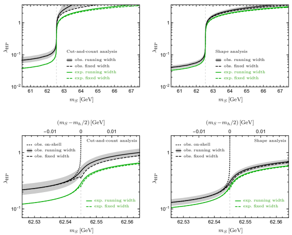
Figure 2: Upper limits at the $95\text{\,}\mathrm{\char 37\relax}$ CL on the Higgs-portal coupling $\lambda_{\text{HP}}$ as a function of the DM mass $m_{S}$. We present results for the cut-and-count analysis (left) and the shape analysis (right) of Ref. Sirunyan:2018owy . We show a wide range for the dark-mater mass (top) as well as a zoom into the most interesting threshold region (bottom). In all plots, we show expected as well es observed limits employing the fixed- and the running-width description for the Higgs propagator. The grey band around the running-width observed limit indicates the $17\text{\,}\mathrm{\char 37\relax}$ uncertainty on the Higgs production cross-section stated in Ref. Sirunyan:2018owy . In the threshold-region plots (bottom), we also indicate the limits due to the decay of an on-shell Higgs boson into DM pairs.

As expected, the approximation of only employing the invisible branching ratio breaks down at threshold, and our analysis derives the proper limits at and above threshold. At $m_{S}=m_{h}/2$ the analysis excludes couplings larger than $\lambda_{\text{HP}}=0.47$ at $95\text{\,}\mathrm{\char 37\relax}$ CL. It can also be seen in Figure 2 that the fixed-width description shows an unphysical feature at threshold. The difference to the running-width results, as expected, becomes less prominent for improved limits, i.e. a smaller Higgs-portal coupling. Hence, in the expected limits the effect is less pronounced than in the observed limit. Well above threshold this difference, which is formally of higher-order in $\lambda_{\text{HP}}$, can be viewed as a lower bound on the theoretical uncertainty. With increasing DM masses the LHC search rapidly looses sensitivity and can only probe large $\lambda_{\text{HP}}$ in the non-perturbative regime.

We also apply Eq. (6) to derive limits from the shape analysis. Here, we assume that the shape of the invariant-mass distribution of the VBF dijet system does not vary substantially with $q^{2}$. Note that relevant limits on the Higgs-portal coupling can only be obtained for DM masses for which the integral in Eq. (6) is dominated by values of $q^{2}$ close to the Higgs mass. The better sensitivity of the shape analysis translates into improved bounds in the Higgs-portal coupling as shown in the right panels of Figure 2. It excludes couplings larger than $\lambda_{\text{HP}}=0.30$ for $m_{S}=m_{h}/2$. However, even the shape analysis cannot constrain perturbative Higgs-portal models for DM masses above $67\text{\,}\mathrm{GeV}$. The effect of the running width is still noticeable in the observed limits. However, the exclusion power of the shape analysis almost pushes the Higgs-portal coupling into a regime where the two prescriptions for the Higgs propagator hardly differ any more.

3.2 Recasting of the cut-and-count analysis

In this section we perform a LO Monte Carlo recasting of the cut-and-count search in Ref. Sirunyan:2018owy , i.e. we compute $\sigma_{h}(q^{2})$ using our Monte Carlo setup and derive $\mu_{\mathcal{H}}^{95\%}(q^{2})$ using Eq. (5) as explained in the following. This allows us to validate our Monte Carlo setup, which is, in particular, needed to obtain projections for the HL-LHC and the HE-LHC in Section 4.

Since no electroweak corrections are included, the off-shell Higgs cross section $\sigma_{h}(q^{2})$ can be obtained by simulating the corresponding on-shell cross section in the SM with different values for the Higgs mass. We generate events with MadGraph5_aMC@NLO v2.6 Alwall:2014hca in the 5-flavor scheme. The renormalization and factorization scales are set to the $W$ mass, $\mu_{R}=\mu_{F}=M_{W}$ deFlorian:2016spz . We use the NNPDF3.0 Ball:2014uwa LO PDF set with $\alpha_{s}(M_{Z})=0.118$ provided by LHAPDF v6.1.6 Buckley:2014ana . The events are subsequently showered and hadronized using Pythia v8.235 Sjostrand:2014zea . Detector simulation is performed with the CMS detector card in Delphes v3.4.2 deFavereau:2013fsa . Jets are clustered with FastJet v3.3.1 Cacciari:2011ma using the anti-kT algorithm Cacciari:2008gp with $R=0.4$. To model the $13\text{\,}\mathrm{TeV}$ CMS VBF analysis Sirunyan:2018owy , we employ the cuts summarized in the corresponding column in Table 1.

Although targeted to select electroweak VBF Higgs production, a subdominant contribution from gluon-initiated Higgs production (associated with two jets) contaminates the search. We estimate this contribution with MadGraph5_aMC@NLO using the HEFT model and reweight Mattelaer:2016gcx the events to the 1-loop level Hirschi:2015iia using the NLO UFO model obtained with NloCT Degrande:2014vpa . We find that gluon fusion contributes with roughly $20\text{\,}\mathrm{\char 37\relax}$ of the VBF production channel. However, the scale uncertainties for gluon fusion are large. Comparing with the gluon-fusion contribution of the more elaborate simulation in Figure 6 of Ref. Sirunyan:2018owy , we find that our simulation overshoots by a factor of two. Hence, the actual gluon-fusion contribution of the $13\text{\,}\mathrm{TeV}$ analysis is not expected to be much bigger than $10\text{\,}\mathrm{\char 37\relax}$. Moreover, using larger dijet invariant mass cuts, the gluon-fusion contribution is expected to be even more suppressed for an analysis at the HL- or HE-LHC. Thus, for simplicity, in the following the gluon-fusion contribution is not simulated explicitly. However, it is indirectly taken into account by a rescaling of our cross section as discussed in the following.

The CMS cut-and-count analysis Ref. Sirunyan:2018owy quotes 743 nominal signal events with an error of 129 events corresponding to a signal cross section (including acceptance times efficiency) of $20.7\text{\,}\mathrm{fb}$. Our simulation of VBF production yields a fiducial cross section of $14.2\text{\,}\mathrm{fb}$ with a scale uncertainty of roughly $25\text{\,}\mathrm{\char 37\relax}$. To improve our LO result, we rescale the LO signal cross section $\sigma_{h}(q^{2})$ by the corresponding factor 1.46 to match the on-shell Higgs-boson cross section in Ref. Sirunyan:2018owy . With this rescaling, we predict $\mu_{\mathcal{H}}$ and compare to Figure 7 of Ref. Sirunyan:2018owy as shown in Figure 3. Up to $m_{\mathcal{H}}=$150\text{\,}\mathrm{GeV}$$ we find agreement below the percent level. Our prediction deviates by $6\text{\,}\mathrm{\char 37\relax}$ at $m_{\mathcal{H}}=$200\text{\,}\mathrm{GeV}$$ and by $14\text{\,}\mathrm{\char 37\relax}$ at $300\text{\,}\mathrm{GeV}$. However, close to the resonance, $m_{S}\lesssim 63\,$GeV, where the 13 TeV analysis is sensitive, the relevant $m_{\mathcal{H}}$ range is confined to be well below $200\text{\,}\mathrm{GeV}$. For DM masses around $70\text{\,}\mathrm{GeV}$ still more than $75\text{\,}\mathrm{\char 37\relax}$ of the cross section arises from contributions with $m_{\mathcal{H}}<$200\text{\,}\mathrm{GeV}$$. Hence, good agreement of our Monte Carlo study with the results in Figure 2 can be expected. We indeed find that the results in Figure 2 are reproduced at the level of the statistical Monte Carlo error not only below but also at and above threshold.

To validate our analysis by an equivalent, independent calculation, for the cut-and-count analysis we also directly simulate DM production with MG5_aMC without making use of $\mu_{\mathcal{H}}^{95\%}(q^{2})$ and Eq. (6). To this end we implement the Higgs-portal model in FeynRules v2.3 Christensen:2008py ; Alloul:2013bka and export it to the UFO format Degrande:2011ua . We use the same signal rescaling factor as above. Note that MG5_aMC only supports fixed-width propagators. We use two different ways to overcome this limitation. On the one hand, we simulate the signal using a fixed width and modify the weight of each event by the respective ratio of the propagators squared. On the other hand, we manipulate the $hSS$ vertex in the UFO model to include the propagator ratio. As to be expected, both approaches give consistent results and agree with the results based on Eq. (6) within MC errors ($\sim$$1\text{\,}\mathrm{\char 37\relax}$) for the event yields.

$\sqrt{s}$	$13\text{\,}\mathrm{TeV}$	$14\text{\,}\mathrm{TeV}$ / $27\text{\,}\mathrm{TeV}$
$p_{T}^{j_{1}}$	$>$80\text{\,}\mathrm{GeV}$$	$>$80\text{\,}\mathrm{GeV}$$
$p_{T}^{j_{2}}$	$>$40\text{\,}\mathrm{GeV}$$	$>$40\text{\,}\mathrm{GeV}$$
$|\eta_{j}|$	$<4.7$	$<5.0$
$\min\left(|\eta_{j_{1}}|,|\eta_{j_{2}}|\right)$	$<3.0$	–
$M_{jj}$	$>$1.3\text{\,}\mathrm{TeV}$$	$>$2.5\text{\,}\mathrm{TeV}$$ / $>$6\text{\,}\mathrm{TeV}$$
$\eta_{j_{1}}\!\cdot\eta_{j_{2}}$	$<0$	$<0$
$|\Delta\eta_{jj}|$	$>4.0$	$>4.0$
$|\Delta\phi_{jj}|$	$<1.5$	$<1.8$
${\not{E}_{T}}$	$>$250\text{\,}\mathrm{GeV}$$	$>$190\text{\,}\mathrm{GeV}$$
$|\Delta\phi_{j{\not{E}_{T}}}|$	$>0.5\ (p_{T}^{j}>$30\text{\,}\mathrm{GeV}$)$	$>0.5\ (p_{T}^{j}>$30\text{\,}\mathrm{GeV}$)$
photon veto	$p_{T}^{\gamma}>$15\text{\,}\mathrm{GeV}$,\ |\eta_{\gamma}|<2.5$	–
electron veto	$p_{T}^{e}>$10\text{\,}\mathrm{GeV}$,\ |\eta_{e}|<2.5$	$p_{T}^{e}>$10\text{\,}\mathrm{GeV}$,\ |\eta_{e}|<2.8$
muon veto	$p_{T}^{\mu}>$10\text{\,}\mathrm{GeV}$,\ |\eta_{\mu}|<2.4$	$p_{T}^{\mu}>$10\text{\,}\mathrm{GeV}$,\ |\eta_{\mu}|<2.8$
$\tau$-lepton veto	$p_{T}^{\tau}>$18\text{\,}\mathrm{GeV}$,\ |\eta_{\tau}|<2.3$	$p_{T}^{\tau}>$20\text{\,}\mathrm{GeV}$,\ |\eta_{\tau}|<3.0$
$b$-jet veto	$p_{T}^{b}>$20\text{\,}\mathrm{GeV}$,\ |\eta_{b}|<2.4$	$p_{T}^{b}>$30\text{\,}\mathrm{GeV}$,\ |\eta_{b}|<5.0$

Table 1: Analysis cuts used in this paper. The cuts for $13\text{\,}\mathrm{TeV}$ and $14\text{\,}\mathrm{TeV}$ are taken from Sirunyan:2018owy and CMS:2018tip , respectively. The cuts for the $27\text{\,}\mathrm{TeV}$ HE-LHC are identical to the ones for the $14\text{\,}\mathrm{TeV}$ HL-LHC except for the cut on $M_{jj}$.

4 HL-LHC and HE-LHC projections

Our HL-LHC projections are based on Ref. CMS:2018tip . For an integrated luminosity of $3\text{\,}{\mathrm{ab}}^{-1}$ at $14\text{\,}\mathrm{TeV}$ center-of-mass energy, the CMS study defines an optimal cut-and-count search by the fiducial phase-space region as shown in Table 1. While the cut on the missing energy has been lowered to $190\text{\,}\mathrm{GeV}$ compared to the $13\text{\,}\mathrm{TeV}$ analysis Sirunyan:2018owy , the higher luminosity allows for raising the dijet invariant mass cut to $2.5\text{\,}\mathrm{TeV}$ in order to increase the signal-to-background ratio while still controlling the background well by data-driven methods.

As in Section 3.1, we make use of the experimental projection in Ref. CMS:2018tip as much as possible, i.e. we employ the cross section and the corresponding event number for all the backgrounds. Moreover, in analogy to Section 3.2, we use the simulated on-shell Higgs-boson production cross section of Ref. CMS:2018tip , which is based on more sophisticated Monte Carlo simulations, to rescale our simulation based on LO Monte Carlo and Delphes. For the $14\text{\,}\mathrm{TeV}$ case, the corresponding rescaling factor is given by 1.54. If we had used the rescaling factor found for the $13\text{\,}\mathrm{TeV}$ analysis in Section 3.2, our prediction for the SM Higgs-production cross section would have deviated from the cross section in Ref. CMS:2018tip by less than $5\text{\,}\mathrm{\char 37\relax}$. Hence, the rescaling factor does not vary substantially with energy and the details of the analysis. We assume that this is also the case for the HE-LHC analysis and will later use the $14\text{\,}\mathrm{TeV}$ rescaling factor also at $27\text{\,}\mathrm{TeV}$.

To obtain our HL-LHC projections we calculate $\sigma_{h}(q^{2})$ with our rescaled LO Monte Carlo simulation and derive the corresponding limit on the signal strength $\mu_{\mathcal{H}}$ as a function of the additional Higgs mass $m_{\mathcal{H}}$. The limit $\mu_{\mathcal{H}}$ is shown as the blue curve in Figure 3. In analogy to Section 3.1, we derive constraints on the Higgs-portal coupling using Eq. (6). The resulting projected limits on the Higgs-portal coupling are shown in Figure 4 as the blue curve. They exclude $\lambda_{\text{HP}}\geq 0.09$ (0.9) for $m_{S}=m_{h}/2$ ($65\text{\,}\mathrm{GeV}$) at $95\text{\,}\mathrm{\char 37\relax}$ CL. As the analysis relies on a data-driven background prediction, its relative systematic uncertainty, $\sigma_{\mathrm{B}}^{\mathrm{sys}}$, is expected to be small. From Ref. CMS:2018tip we derive $\sigma_{\mathrm{B}}^{\mathrm{sys}}=$1.4\text{\,}\mathrm{\char 37\relax}$$ (see below for more details). We indicate the dependence on the systematic uncertainties of the background prediction by the blue shaded band, for which we vary $\sigma_{\mathrm{B}}^{\mathrm{sys}}$ by a factor of 2. Note that the expected limit of the high-luminosity cut-and-count analysis supersedes the observed limits from the $13\text{\,}\mathrm{TeV}$ shape analysis already for a systematic uncertainty below $12\text{\,}\mathrm{\char 37\relax}$. Of course, a more sophisticated (shape-like) analysis is expected to even further improve the limits as for the $13\text{\,}\mathrm{TeV}$ search.

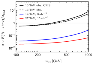
Figure 3: $95\text{\,}\mathrm{\char 37\relax}$ CL upper limit on $\mu_{\mathcal{H}}=\sigma\times{\cal B}({\cal H}\to\text{inv})/\sigma_{\text{SM}}$ for an additional SM-like Higgs boson ${\cal H}$ that does not mix with the SM Higgs boson as a function of its mass, $m_{\cal H}$. The black solid curve shows the existing limit from CMS reported in Ref. Sirunyan:2018owy while the black dashed curve shows our limit from the recasting of this search. The blue and red curves show our projected limits for the $14\text{\,}\mathrm{TeV}$ HL-LHC and $27\text{\,}\mathrm{TeV}$ HE-LHC, respectively.

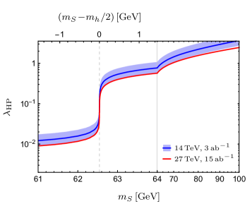
Figure 4: Projected $95\text{\,}\mathrm{\char 37\relax}$ CL upper limits on the Higgs-portal coupling for the $14\text{\,}\mathrm{TeV}$ HL-LHC (blue curve) and $27\text{\,}\mathrm{TeV}$ HE-LHC (red curve) assuming an integrated luminosity of $3\text{\,}{\mathrm{ab}}^{-1}$ and $15\text{\,}{\mathrm{ab}}^{-1}$, respectively. The shaded band around the blue curve indicates the sensitivity of the respective limit to the systematic error on the background from Ref. CMS:2018tip which is multiplied by a factor of 2 (1/2) for the upper (lower) boundary of the band. To resolve the resonant region, for the abscissa we impose a scale break at a DM mass of $64\text{\,}\mathrm{GeV}$, below (above) which we plot the mass linearly (logarithmically).

To evaluate the potential of the HE-LHC, we now turn to projections for a $27\text{\,}\mathrm{TeV}$ machine. Since there is no corresponding experimental projection for a $27\text{\,}\mathrm{TeV}$ HE-LHC option, we simulate the dominating backgrounds and estimate the respective error which is most crucial to assess the sensitivity of the search. To this end we exploit the corresponding information provided in the $14\text{\,}\mathrm{TeV}$ HL-LHC projection CMS:2018tip as explained in the following. We generate the leading background processes $pp\to Z+\text{jets}$ and $pp\to W^{\pm}+\text{jets}$ for $14\text{\,}\mathrm{TeV}$ at LO using MG5_aMC and employ the MLM matching scheme alwall-2008-53 to merge samples with 2 and 3 jets. We separately simulate processes with jets produced through electroweak (EW) interactions and processes in which all jets originate from QCD radiation, neglecting interference between the two. The detector response is simulated using the HL-LHC detector card in Delphes. To improve our LO background calculation in analogy with our signal prediction, we determine rescaling factors for each background process by comparing the cross sections (including acceptance times efficiency) to the cross sections reported in Ref. CMS:2018tip . By rescaling to the results in Ref. CMS:2018tip , we profit both from the more elaborate background simulation and the more sophisticated simulation of detector effects in the experimental projection. We include the subleading top-contribution (below $4\text{\,}\mathrm{\char 37\relax}$) in the rescaling factor for the $W$ backgrounds assuming a roughly similar $M_{jj}$ dependence. We then simulate the various backgrounds at $27\text{\,}\mathrm{TeV}$ and perform a rescaling for each channel with the rescaling factors determined at $14\text{\,}\mathrm{TeV}$. The corresponding $M_{jj}$ distributions are shown in Figure 5.

Given the large statistics, the systematic uncertainty for the background prediction is crucial for the sensitivity of the corresponding search. The background prediction at a $27\text{\,}\mathrm{TeV}$ HE-LHC in the experimental search will be data driven using control regions as it is the case for the $13\text{\,}\mathrm{TeV}$ search discussed in Section 3 and in the $14\text{\,}\mathrm{TeV}$ HL-LHC projection. For example, the background due to $Z$-boson production, where the $Z$ bosons decay into neutrinos, can be measured to a large extent by $Z$-boson decays into charged leptons in a control region. Due to the smaller branching ratio into charged leptons, this measurement has smaller statistics. The corresponding statistical error scales like the square root of the number of events in the control region. In addition, there is always a relative systematic error that does not scale with the integrated luminosity and arises from relating the control-region measurements to the signal-region background estimate. We denote this luminosity-independent error by $\sigma_{\mathrm{B}}^{\mathrm{ind}}$. While a full account of this procedure is clearly beyond the scope of this work and can only be performed in the experimental analysis, the above discussion motivates the following simple modeling for the relative systematic error $\sigma_{\mathrm{B}}^{\mathrm{sys}}$ of the background prediction according to

$$\sigma_{\mathrm{B}}^{\mathrm{sys}}=\sqrt{f/N_{\text{B}}+(\sigma_{\mathrm{B}}^{\mathrm{ind}})^{2}}\,,$$ (9)

where $N_{\text{B}}$ is the number of background events in the signal region and the parameter $f$ reflects the fact that the control-region measurement potentially has smaller statistics (in which case $f>1$) but still scales like a statistical error with increasing luminosity. Hence, the $95\text{\,}\mathrm{\char 37\relax}$ CL expected limit for the number of signal events $N_{\text{S}}$ can be obtained in the asymptotic (Gaussian) limit from

$$\frac{N_{\text{S}}}{\sqrt{N_{\text{B}}+\left(\sigma_{\mathrm{B}}^{\mathrm{sys}}N_{\text{B}}\right)^{2}+N_{\text{S}}}}=1.96\,.$$ (10)

To obtain realistic estimates for $f$ and $\sigma_{\mathrm{B}}^{\mathrm{ind}}$, we use the $14\text{\,}\mathrm{TeV}$ projection. As $N_{\text{S}}$ and $N_{\text{B}}$ scale with the integrated luminosity we use the limit for the invisible branching ratio for the three different luminosities provided in Figure 5 of Ref. CMS:2018tip to determine $f=1.5$ and $\sigma_{\mathrm{B}}^{\mathrm{ind}}=$1.3\text{\,}\mathrm{\char 37\relax}$$. Using these values, our simple modeling of the systematic error nicely reproduces the results in Figure 5 of Ref. CMS:2018tip . We use these numbers as the best estimate parametrising the background uncertainty for the HE-LHC projection.

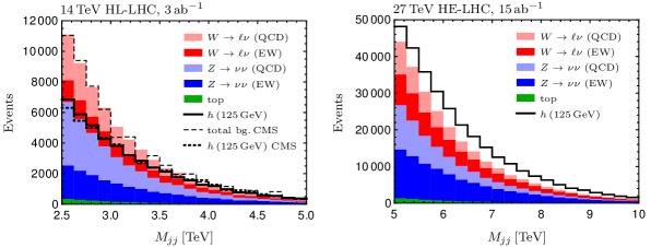
Figure 5: Binned $M_{jj}$ distributions for our background (stacked histograms) and signal (thick solid line) prediction for the $14\text{\,}\mathrm{TeV}$ HL-LHC (left panel) and $27\text{\,}\mathrm{TeV}$ HE-LHC (right panel). Apart from $M_{jj}$, the analysis cuts listed in Table 1 are applied. For comparison, we show the total background (thin dashed line) and signal (thick dotted line) predictions for the $14\text{\,}\mathrm{TeV}$ HL-LHC from CMS as reported in Ref. CMS:2018tip .

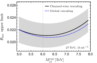
Figure 6: Upper limit on the invisible branching ratio of the SM Higgs boson as a function of the $M_{jj}$-cut for the $27\text{\,}\mathrm{TeV}$ HE-LHC. Otherwise cuts from Tab. 1 are applied. We show the limit using a channel-wise (black, solid) and global (blue, dotted) rescaling of the background prediction, see text for details. For illustration, the grey band shows the respective shift of the solid black line resulting from a $10\text{\,}\mathrm{\char 37\relax}$ variation of the background cross section.

Optimizing the cut-and-count search for a $27\text{\,}\mathrm{TeV}$ machine, we find the biggest potential for gaining sensitivity in strengthening the cut on $M_{jj}$, while we leave all other cuts as in the $14\text{\,}\mathrm{TeV}$ analysis. In order to obtain an estimate for the optimal $M_{jj}$-cut at $27\text{\,}\mathrm{TeV}$ we employ the following strategy. Producing a high-statistics sample with a detector-level $M_{jj}$-cut at $5\text{\,}\mathrm{TeV}$ we find the $M_{jj}$ distribution shown in the right panel of Figure 5, which allows us to compute the total number of background events as a function of a given $M_{jj}$-cut. Furthermore, we simulate a high-statistics sample for on-shell SM Higgs production assuming $100\text{\,}\mathrm{\char 37\relax}$ invisible branching ratio. The resulting branching ratio limit as a function of $M_{jj}$ is shown in Figure 6. For comparison, we also show the result using a global rescaling factor, i.e. rescaling all simulated background contributions with the same factor instead of rescaling each background channel individually. This global rescaling factor is chosen such that the two background estimates coincide for a $M_{jj}$-cut at $5\text{\,}\mathrm{TeV}$. The small difference between a global and channel-wise rescaling is an indicator for the robustness of the $M_{jj}$ dependence of our background estimate. We find that the upper limit on the invisible branching ratio is strongest at $M_{jj}$-cuts around $6\text{\,}\mathrm{TeV}6.5\text{\,}\mathrm{TeV}$, with little sensitivity on the detailed choice. We adopt the value $M_{jj}>$6\text{\,}\mathrm{TeV}$$. For this choice, the relative uncertainty of the background $\sigma_{\mathrm{B}}^{\mathrm{sys}}=$1.4\text{\,}\mathrm{\char 37\relax}$$ for an integrated luminosity of $15\text{\,}{\mathrm{ab}}^{-1}$ is already dominated by $\sigma_{\mathrm{B}}^{\mathrm{ind}}$.

Note that the uncertainty of our LO Monte Carlo simulation in the prediction of the background yield is large, around $10\!-\!$20\text{\,}\mathrm{\char 37\relax}$$, which translates into a shift in the limits by roughly the same amount (see Figure 6). However, this uncertainty disappears, of course, once data has been taken, i.e. the data-driven background prediction is made.

Using the above input on the background prediction and the corresponding error estimate, we calculate $\sigma_{h}(q^{2})$ with our rescaled LO Monte Carlo simulation as before and derive the corresponding limit on the signal strength $\mu_{\mathcal{H}}$ shown in Figure 3. For the SM Higgs with $m_{h}\simeq$125\text{\,}\mathrm{GeV}$$ the projected HE-LHC $95\text{\,}\mathrm{\char 37\relax}$ CL upper limit on the invisible branching ratio is 0.021. The resulting limits on the Higgs-portal coupling are shown in Figure 4. For $m_{S}\lesssim$61\text{\,}\mathrm{GeV}$$ the Higgs portal coupling is expected to be constrained to less than $\lambda_{\text{HP}}=0.01$, while at the resonance $m_{S}=m_{h}/2$ we find $\lambda_{\text{HP}}<0.077$. Useful (perturbative) limits can be obtained up to DM masses of $110\text{\,}\mathrm{GeV}$. These limits can be viewed as conservative. Improving the systematic uncertainty in the background prediction or using more sophisticated shape-like or multivariate techniques might further strengthen the limits.

5 Conclusion

We have conducted a dedicated study of scalar Higgs-portal DM in the VBF channel, presenting limits from current LHC data as well as projections for the HL- and HE-LHC upgrades. Results for other types of Higgs-portal DM candidates are included in Appendix B. Due to its distinct topology, the VBF channel provides particularly promising prospects to probe this kind of models. The analysis is based on the VBF search for invisible Higgs decays Sirunyan:2018owy and the corresponding high-luminosity forecast CMS:2018tip by CMS. Our projected sensitivities include an estimate of the systematic uncertainty that can be achieved with a data-driven background prediction.

Special focus has been put on the DM mass region $m_{S}\simeq m_{h}/2$ as this region is particularly well-motivated due to constraints from the DM abundance and direct detection. If the mass of DM is slightly too large for being produced via an on-shell Higgs boson, the invisible channel opens up within the Higgs-boson resonance. This gives rise to an unphysical enhancement of the cross section if the total Higgs-boson width is kept fixed in the propagator. We solve this problem by using a running-width prescription. For the observed limits on the Higgs-portal coupling, the fixed-width prescription over-estimates the constraining power of the cut-and-count (shape) analysis by up to roughly $30\text{\,}\mathrm{\char 37\relax}$ ($15\text{\,}\mathrm{\char 37\relax}$). Note that an effect of similar size would also be present in the annihilation cross section relevant for the computation of the freeze-out abundance, if similarly large couplings were considered.

We obtain a $95\text{\,}\mathrm{\char 37\relax}$ CL upper limit on the Higgs invisible branching ratio of 0.021 at the HE-LHC with $15\text{\,}{\mathrm{ab}}^{-1}$. The corresponding $1314\text{\,}\mathrm{TeV}$ limits are 0.3 Sirunyan:2018owy and 0.038 CMS:2018tip , respectively. With current LHC data, Higgs-portal couplings of the order of $\lambda_{\text{HP}}\simeq 0.04$ (at $m_{S}=$61\text{\,}\mathrm{GeV}$$) can be excluded below threshold. At $m_{S}=m_{h}/2$ the LHC probes $\lambda_{\text{HP}}\simeq 0.3$, whereas above the threshold only couplings as large as $\lambda_{\text{HP}}\simeq 2.5$ (at $m_{S}=$64\text{\,}\mathrm{GeV}$$) can be reached. With an integrated luminosity of $3\text{\,}{\mathrm{ab}}^{-1}$ collected at the HL-LHC the corresponding limits improve to $\lambda_{\text{HP}}\simeq 0.01,\ 0.09,\ \text{and}\ 0.8$, respectively. At the HE-LHC with $15\text{\,}{\mathrm{ab}}^{-1}$ we estimate a further improvement of these bounds by roughly $30\text{\,}\mathrm{\char 37\relax}$. Stronger limits may be achieved employing analysis techniques beyond a simple cut-and-count analysis and/or by improving the systematic uncertainty.

Following Ref. Sirunyan:2018owy , we also present our HL- and HE-LHC results as upper limits on the signal strength $\mu_{\mathcal{H}}$ of an invisibly decaying, SM-like Higgs boson with mass $m_{\mathcal{H}}$. We find that at the HL-LHC (HE-LHC) $\mu_{\mathcal{H}}$ can be constrained to values better than $\mu_{\mathcal{H}}<0.1$ for masses below $m_{\mathcal{H}}\lesssim$500\text{\,}\mathrm{GeV}$\ ($1\text{\,}\mathrm{TeV}$)$. These limits allow for a simple reinterpretation for other Higgs-mediated DM models using Eq. (6). All results can be found in digital form in the supplementary material to this paper.

Appendix A Threshold at a resonance

It is common to use a fixed-width prescription for the resonant Higgs propagator, i.e.

$$P_{\text{f}}(q^{2})=\frac{\mathrm{i}}{q^{2}-m_{h}^{2}+\mathrm{i}\,m_{h}\,\Gamma_{\mathrm{tot}}(m_{h}^{2})}\,,$$ (11)

where $m_{h}$ is the Higgs-boson mass and $\Gamma_{\mathrm{tot}}(m_{h}^{2})$ is the total width of an on-shell Higgs boson. The production rate of all Higgs-boson decay modes via a resonant Higgs boson is then given by

$$\sigma^{\mathrm{tot}}_{\text{f}}=\int\frac{\mathrm{d}q^{2}}{2\pi}\,\sigma_{h}(q^{2})\,\frac{2q\Gamma_{\mathrm{tot}}(q^{2})}{\left(q^{2}-m_{h}^{2}\right)^{2}+m_{h}^{2}\Gamma_{\mathrm{tot}}^{2}(m_{h}^{2})}\,,$$ (12)

where $\sigma_{h}(q^{2})$ is the production cross-section for a given Higgs-boson invariant mass $q^{2}$. The integral is dominated by the on-shell region $q^{2}\sim m_{h}^{2}$ which has a width of $\mathcal{O}(m_{h}\Gamma_{\mathrm{tot}})$. Hence, if $\Gamma_{\mathrm{tot}}(m_{h}^{2})$ is small and $\sigma_{h}(q^{2})$ as well as $\Gamma_{\mathrm{tot}}(q^{2})$ are smooth functions, the narrow-width approximation

$$\sigma^{\mathrm{tot}}_{\text{f}}\simeq\int\frac{\mathrm{d}q^{2}}{2\pi}\,\sigma_{h}(m_{h}^{2})\,\frac{2m_{h}\Gamma_{\mathrm{tot}}(m_{h}^{2})}{\left(q^{2}-m_{h}^{2}\right)^{2}+m_{h}^{2}\Gamma_{\mathrm{tot}}^{2}(m_{h}^{2})}=\sigma_{h}(m_{h}^{2})$$ (13)

is valid. However, if the total width $\Gamma_{\mathrm{tot}}(q^{2})$ is a rapidly varying function in the resonance region, the fixed width prescription for the propagator and the narrow-width approximation may break down. In particular, if a new decay channel with a large coupling opens up close to the resonance, the increase in $\Gamma_{\mathrm{tot}}(q^{2})$ leads to a large increase of $\sigma^{\mathrm{tot}}_{\text{f}}$ if it is calculated using Eq. (12). Hence, $\sigma^{\mathrm{tot}}_{\text{f}}$ is not related any more to the production cross section $\sigma_{h}(m_{h}^{2})$ as it should be.

To illustrate the issue, one can use the narrow-width approximation for the production cross section and investigate the ratio

$$R_{\text{f}}^{\mathrm{tot}}=\int\frac{\mathrm{d}q^{2}}{2\pi}\,\frac{2q\Gamma_{\mathrm{tot}}(q^{2})}{\left(q^{2}-m_{h}^{2}\right)^{2}+m_{h}^{2}\Gamma_{\mathrm{tot}}^{2}(m_{h}^{2})}\simeq\frac{\sigma^{\mathrm{tot}}_{\text{f}}}{\sigma_{h}(m_{h}^{2})}\,.$$ (14)

In the following, we use the tree-level width for the Higgs decay into two singlets

$$\Gamma_{\text{inv}}(q^{2})=\frac{\lambda_{\text{HP}}^{2}}{32\pi}\frac{v^{2}}{q}\sqrt{1-\frac{4m_{S}^{2}}{q^{2}}}\,\Theta(q^{2}-4m_{S}^{2})\,$$ (15)

to define the total width $\Gamma_{\mathrm{tot}}(q^{2})=\Gamma_{\mathrm{vis}}+\Gamma_{\text{inv}}(q^{2})$, where $\Gamma_{\mathrm{vis}}$ is the Higgs width in the SM. We neglect the $q^{2}$ dependence of $\Gamma_{\mathrm{vis}}$ as the dominant effect comes from the invisible part. Figure 7 shows the ratio $R_{f}^{\mathrm{tot}}$ as a function of the singlet mass $m_{S}$. If the invisible decay channel into singlets opens up in the vicinity of the Higgs-boson resonance, the description is clearly unphysical since $R_{\text{f}}^{\mathrm{tot}}$ can become large.

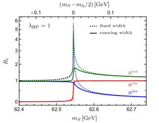
Figure 7: Cross section ratios $R_{\text{f}}\approx\frac{\sigma_{\text{f}}}{\sigma_{h}(m_{h}^{2})}$ (dashed lines) and $R_{\text{r}}\approx\frac{\sigma_{\text{r}}}{\sigma_{h}(m_{h}^{2})}$ (solid lines) using a fixed- and a running-width prescription for the Higgs-boson propagator, respectively. We consider the ratios $R^{\mathrm{tot}}$ w.r.t. the total cross section (black), $R^{\mathrm{vis}}$ w.r.t. the SM Higgs-decay products (red) and $R^{\mathrm{inv}}$ w.r.t. the Higgs decay into singlets (blue). This plot is obtained for $\lambda_{\text{HP}}=1$.

The obvious improvement is to use a running-width prescription in the Higgs propagator according to

$$P_{\text{r}}(q^{2})=\frac{\mathrm{i}}{q^{2}-m_{S}^{2}+\mathrm{i}\sqrt{q^{2}}\,\Gamma_{\mathrm{tot}}(q^{2})}\,.$$ (16)

The ratio

$$R_{\text{r}}^{\mathrm{tot}}=\int\frac{\mathrm{d}q^{2}}{2\pi}\,\frac{2q\Gamma_{\mathrm{tot}}(q^{2})}{\left(q^{2}-m_{h}^{2}\right)^{2}+q^{2}\Gamma_{\mathrm{tot}}^{2}(q^{2})}\approx\frac{\sigma^{\mathrm{tot}}_{\text{r}}}{\sigma_{h}(m_{h}^{2})}$$ (17)

is well behaved as can be seen in Figure 7. In particular, if the total cross section is written as the sum of the production cross-section of all SM final-states $\sigma^{\mathrm{vis}}$ and the singlet final-state $\sigma^{\mathrm{inv}}$ the physics interpretation of the results becomes transparent. If the decay channel to singlets is already open at the Higgs-boson resonance, it dominates for large coupling and almost all the produced Higgs bosons decay into the invisible channel. If, on the other hand, the decay channel to singlets is not open, $\sigma^{\mathrm{vis}}$ is almost unchanged with respect to the SM and there is additional off-shell production of the singlet final-state. In the resonance region, the running width in the Higgs propagator leads to a smooth transition between the on-shell and the off-shell production of the singlet final-state $\sigma^{\mathrm{inv}}$ as shown in Figure 7.

Appendix B Fermion, vector and tensor dark matter

In this appendix we derive $95\text{\,}\mathrm{\char 37\relax}$ CL upper limits on the Higgs portal coupling for other choices of DM particles. We consider the interaction Lagrangians (before electroweak symmetry breaking)

$$\mathcal{L}_{\text{HP}}=-\frac{\lambda_{\text{HP}}}{\Lambda}\Phi^{\dagger}\Phi\overline{\chi}\chi$$ (18a)

for a Majorana fermion $$\chi$$,

$$\mathcal{L}_{\text{HP}}=-\frac{\lambda_{\text{HP}}}{2}\,\Phi^{\dagger}\Phi\,X^{\mu}X_{\mu}$$ (18b)

for a vector $$X$$, and

$$\mathcal{L}_{\text{HP}}=-\frac{\lambda_{\text{HP}}}{2}\,\Phi^{\dagger}\Phi\,B^{\mu\nu}B_{\mu\nu}$$ (18c)

for an anti-symmetric rank-2 tensor $B$. More details about the models can be found in Kanemura:2010sh ; Endo:2014cca ; Cata:2014sta . For the tensor model, we follow the conventions of Ref. Cata:2014sta . The Higgs-portal interaction leads to the following expressions for the invisible Higgs-boson width Kanemura:2010sh ; Endo:2014cca :

$$\Gamma\left(h\rightarrow\chi\overline{\chi}\right)= \ \frac{\lambda_{\text{HP}}^{2}v^{2}}{4\pi\Lambda^{2}}m_{h}\left(1-\frac{4m_{\chi}^{2}}{m_{h}^{2}}\right)^{3/2},$$ (19a)

$$\Gamma\left(h\rightarrow XX\right)= \ \frac{\lambda_{\text{HP}}^{2}}{128\pi}\frac{v^{2}}{m_{h}}\frac{m_{h}^{4}-4m_{h}^{2}m_{X}^{2}+12m_{X}^{4}}{m_{X}^{4}}\sqrt{1-\frac{4m_{X}^{2}}{m_{h}^{2}}},$$ (19b)

$$\Gamma\left(h\rightarrow BB\right)= \ \frac{\lambda_{\text{HP}}^{2}}{16\pi}\frac{v^{2}}{m_{h}}\frac{m_{h}^{4}-4m_{h}^{2}m_{B}^{2}+6m_{B}^{4}}{m_{B}^{4}}\sqrt{1-\frac{4m_{B}^{2}}{m_{h}^{2}}}.$$ (19c)

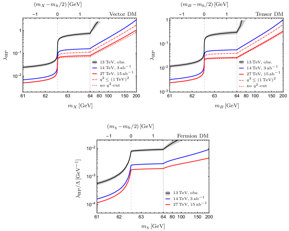
Figure 8: $95\text{\,}\mathrm{\char 37\relax}$ CL upper limits on the Higgs-portal coupling for the case of vector (upper left), tensor (upper right) and Majorana fermion DM (lower panel). The black curve (and grey band) denotes the $13\text{\,}\mathrm{TeV}$ LHC observed limit (and the signal uncertainty). The blue and red curves denote the $14\text{\,}\mathrm{TeV}$ HL- and $27\text{\,}\mathrm{TeV}$ HE-LHC projections, respectively. For the vector and tensor models, we use a cut-off for the integral in Eq. (6) as discussed in the text. The dashed and dotted light red curves indicate the HE-LHC limits if a $1\text{\,}\mathrm{TeV}$ cut-off or no cut-off is used instead, respectively. To resolve the resonant region, for the abscissa we impose a scale break at a DM mass of $64\text{\,}\mathrm{GeV}$, below (above) which we plot the mass linearly (logarithmically).

In contrast to the case of singlet scalar DM treated in the main text, the models in Eq. (18) considered in this appendix are not UV complete. They are non-renormalizable and violate perturbative unitarity at high energies. As a consequence, the DM production cross section Eq. (4) receives large contributions from $q^{2}\gg m_{\text{DM}}^{2}$. For example, it is well known from vector-boson scattering in the SM that perturbative unitarity is violated at $q^{2}\sim($1\text{\,}\mathrm{TeV}$)^{2}$ for $m_{X}\sim m_{Z}$ and a coupling $\lambda_{\text{HP}}$ of weak size Lee:1977eg . The unitarity violating contributions are, however, expected to be suppressed in UV-completions of the models, e.g. via additional degrees of freedom that unitarize the theory. To exclude the potentially unitarity-violating high-energy contribution, we derive the unitarity limit from $hh\to XX$ scattering at $\mathcal{O}(\lambda_{\text{HP}})$ Lebedev:2011iq and cut off the integral in Eq. (4) at $q^{2}=32\pi m_{X}^{2}/\lambda_{\text{HP}}$ for the vector case. In analogy, we use $q^{2}=16\pi m_{B}^{2}/\lambda_{\text{HP}}$ in the tensor case. Note that in the vector and tensor model for $m_{X,B}>m_{h}/2$ the limits depend approximately linearly on the choice of the cut-off near $q^{2}=($1\text{\,}\mathrm{TeV}$)^{2}$. Figure 8 therefore also shows the HE-LHC limits obtained for a cut-off at $1\text{\,}\mathrm{TeV}$ (dashed) as a conservative limit and without cut-off (dotted). For the fermion case, a strong cut-off dependence is absent and we do not employ a cut-off. Note that we use the running-width prescription which has a unitarizing effect (see also Ref. Khoze:2017tjt ) if the total width becomes so large that it dominates the denominator of the Higgs-boson propagator. This is also the reason why the $13\text{\,}\mathrm{TeV}$ exclusion lines in the vector and tensor case stop around $m_{X/B}=$75\text{\,}\mathrm{GeV}$$. The cross-section reaches a maximum for a certain value of $\lambda_{\text{HP}}$ and decreases again for larger couplings. To establish limits in this region of parameter space, the high-energy behaviour of the models needs to be studied in more detail which is beyond the scope of this work.

Using the method of Sec. 3.1 we compute the limit on $\lambda_{\text{HP}}$ within the three models. Figure 8 shows the respective observed $13\text{\,}\mathrm{TeV}$ LHC limit from the shape analysis (black curves) as well as the projections for the $14\text{\,}\mathrm{TeV}$ HL-LHC and $27\text{\,}\mathrm{TeV}$ HE-LHC, respectively. The grey band around the $13\text{\,}\mathrm{TeV}$ limit denotes the signal uncertainty, see Sec. 3.1. In the vector model, current data excludes couplings around $\lambda_{\text{HP}}\simeq 0.03\ (0.7)$ slightly below (above) the threshold, whereas the corresponding limits in the tensor model are smaller by about a factor of 2. At $m_{\text{DM}}=m_{h}/2$, $\lambda_{\text{HP}}=0.17\ (0.08)$ is excluded in the vector (tensor) case. For fermionic DM, $\lambda_{\text{HP}}/\Lambda\simeq$0.510\text{\,}{\mathrm{TeV}}^{-1}$$ ($\lambda_{\text{HP}}/\Lambda=$8.0\text{\,}{\mathrm{TeV}}^{-1}$$) can be probed for $m_{\chi}\lesssim$65\text{\,}\mathrm{GeV}$\ (m_{\chi}=m_{h}/2)$. The HL- and HE-LHC improve these bounds by a factor of 3 to 10.

References

- (1) J. Silk et al., Particle Dark Matter: Observations, Models and Searches. Cambridge Univ. Press, Cambridge, 2010. 10.1017/CBO9780511770739.
- (2) V. Silveira and A. Zee, Scalar Phantoms, Phys. Lett. B161 (1985) 136.
- (3) J. McDonald, Gauge singlet scalars as cold dark matter, Phys. Rev. D50 (1994) 3637–3649, [hep-ph/0702143].
- (4) C. P. Burgess, M. Pospelov and T. ter Veldhuis, The Minimal model of nonbaryonic dark matter: A Singlet scalar, Nucl. Phys. B619 (2001) 709–728, [hep-ph/0011335].
- (5) Y. G. Kim, K. Y. Lee and S. Shin, Singlet fermionic dark matter, JHEP 05 (2008) 100, [0803.2932].
- (6) L. Lopez-Honorez, T. Schwetz and J. Zupan, Higgs portal, fermionic dark matter, and a Standard Model like Higgs at 125 GeV, Phys. Lett. B716 (2012) 179–185, [1203.2064].
- (7) S. Baek, P. Ko, W.-I. Park and E. Senaha, Higgs Portal Vector Dark Matter: Revisited, JHEP 05 (2013) 036, [1212.2131].
- (8) D. G. E. Walker, Unitarity Constraints on Higgs Portals, 1310.1083.
- (9) A. Freitas, S. Westhoff and J. Zupan, Integrating in the Higgs Portal to Fermion Dark Matter, JHEP 09 (2015) 015, [1506.04149].
- (10) T. Binder, T. Bringmann, M. Gustafsson and A. Hryczuk, Early kinetic decoupling of dark matter: when the standard way of calculating the thermal relic density fails, Phys. Rev. D96 (2017) 115010, [1706.07433].
- (11) K. Ala-Mattinen and K. Kainulainen, Precision calculations of dark matter relic abundance, 1912.02870.
- (12) GAMBIT collaboration, P. Athron et al., Status of the scalar singlet dark matter model, Eur. Phys. J. C77 (2017) 568, [1705.07931].
- (13) P. Athron, J. M. Cornell, F. Kahlhoefer, J. Mckay, P. Scott and S. Wild, Impact of vacuum stability, perturbativity and XENON1T on global fits of and scalar singlet dark matter, Eur. Phys. J. C78 (2018) 830, [1806.11281].
- (14) XENON collaboration, E. Aprile et al., Dark Matter Search Results from a One Ton-Year Exposure of XENON1T, Phys. Rev. Lett. 121 (2018) 111302, [1805.12562].
- (15) L. Feng, S. Profumo and L. Ubaldi, Closing in on singlet scalar dark matter: LUX, invisible Higgs decays and gamma-ray lines, JHEP 03 (2015) 045, [1412.1105].
- (16) A. Cuoco, B. Eiteneuer, J. Heisig and M. Krämer, A global fit of the -ray galactic center excess within the scalar singlet Higgs portal model, JCAP 1606 (2016) 050, [1603.08228].
- (17) A. Cuoco, J. Heisig, M. Korsmeier and M. Krämer, Probing dark matter annihilation in the Galaxy with antiprotons and gamma rays, JCAP 1710 (2017) 053, [1704.08258].
- (18) B. Eiteneuer, A. Goudelis and J. Heisig, The inert doublet model in the light of Fermi-LAT gamma-ray data: a global fit analysis, Eur. Phys. J. C77 (2017) 624, [1705.01458].
- (19) C. Arina, A. Beniwal, C. Degrande, J. Heisig and A. Scaffidi, Global fit of pseudo-Nambu-Goldstone Dark Matter, 1912.04008.
- (20) M. Garny, J. Heisig, B. Lülf and S. Vogl, Coannihilation without chemical equilibrium, Phys. Rev. D96 (2017) 103521, [1705.09292].
- (21) R. T. D’Agnolo, D. Pappadopulo and J. T. Ruderman, Fourth Exception in the Calculation of Relic Abundances, Phys. Rev. Lett. 119 (2017) 061102, [1705.08450].
- (22) T. N. Maity and T. S. Ray, Exchange driven freeze out of dark matter, 1908.10343.
- (23) M. Kamionkowski and M. S. Turner, Thermal relics: Do we know their abundances?, Phys. Rev. D42 (1990) 3310–3320.
- (24) C. Gross, O. Lebedev and T. Toma, Cancellation Mechanism for Dark-Matter-Nucleon Interaction, Phys. Rev. Lett. 119 (2017) 191801, [1708.02253].
- (25) J. A. Casas, D. G. Cerdeño, J. M. Moreno and J. Quilis, Reopening the Higgs portal for single scalar dark matter, JHEP 05 (2017) 036, [1701.08134].
- (26) S. Bhattacharya, P. Ghosh, T. N. Maity and T. S. Ray, Mitigating Direct Detection Bounds in Non-minimal Higgs Portal Scalar Dark Matter Models, JHEP 10 (2017) 088, [1706.04699].
- (27) D. R. T. Jones and S. T. Petcov, Heavy Higgs Bosons at LEP, Phys. Lett. 84B (1979) 440–444.
- (28) R. N. Cahn and S. Dawson, Production of Very Massive Higgs Bosons, Phys. Lett. 136B (1984) 196.
- (29) O. J. P. Eboli and D. Zeppenfeld, Observing an invisible Higgs boson, Phys. Lett. B495 (2000) 147–154, [hep-ph/0009158].
- (30) N. Craig, H. K. Lou, M. McCullough and A. Thalapillil, The Higgs Portal Above Threshold, JHEP 02 (2016) 127, [1412.0258].
- (31) M. Endo and Y. Takaesu, Heavy WIMP through Higgs portal at the LHC, Phys. Lett. B743 (2015) 228–234, [1407.6882].
- (32) H. Han, J. M. Yang, Y. Zhang and S. Zheng, Collider Signatures of Higgs-portal Scalar Dark Matter, Phys. Lett. B756 (2016) 109–112, [1601.06232].
- (33) D. Dercks and T. Robens, Constraining the Inert Doublet Model using Vector Boson Fusion, Eur. Phys. J. C79 (2019) 924, [1812.07913].
- (34) G. Arcadi, A. Djouadi and M. Raidal, Dark Matter through the Higgs portal, 1903.03616.
- (35) C. Bernaciak, T. Plehn, P. Schichtel and J. Tattersall, Spying an invisible Higgs boson, Phys. Rev. D91 (2015) 035024, [1411.7699].
- (36) D. Goncalves, T. Plehn and J. M. Thompson, Weak boson fusion at 100 TeV, Phys. Rev. D95 (2017) 095011, [1702.05098].
- (37) A. Biekötter, F. Keilbach, R. Moutafis, T. Plehn and J. Thompson, Tagging Jets in Invisible Higgs Searches, SciPost Phys. 4 (2018) 035, [1712.03973].
- (38) D. Buttazzo, D. Redigolo, F. Sala and A. Tesi, Fusing Vectors into Scalars at High Energy Lepton Colliders, JHEP 11 (2018) 144, [1807.04743].
- (39) CMS collaboration, A. M. Sirunyan et al., Search for invisible decays of a Higgs boson produced through vector boson fusion in proton-proton collisions at 13 TeV, Phys. Lett. B793 (2019) 520–551, [1809.05937].
- (40) ATLAS collaboration, M. Aaboud et al., Search for invisible Higgs boson decays in vector boson fusion at TeV with the ATLAS detector, Phys. Lett. B793 (2019) 499–519, [1809.06682].
- (41) M. Ruhdorfer, E. Salvioni and A. Weiler, A Global View of the Off-Shell Higgs Portal, 1910.04170.
- (42) CMS collaboration, A. M. Sirunyan et al., Search for invisible decays of a Higgs boson produced through vector boson fusion at the High-Luminosity LHC, CMS-PAS-FTR-18-016.
- (43) T. Junk, Confidence level computation for combining searches with small statistics, Nucl. Instrum. Meth. A434 (1999) 435–443, [hep-ex/9902006].
- (44) A. L. Read, Presentation of search results: The CL(s) technique, J. Phys. G28 (2002) 2693–2704.
- (45) https://www.hepdata.net.
- (46) G. Belanger, B. Dumont, U. Ellwanger, J. F. Gunion and S. Kraml, Global fit to Higgs signal strengths and couplings and implications for extended Higgs sectors, Phys. Rev. D88 (2013) 075008, [1306.2941].
- (47) S. Kraml, T. Q. Loc, D. T. Nhung and L. D. Ninh, Constraining new physics from Higgs measurements with Lilith: update to LHC Run 2 results, SciPost Phys. 7 (2019) 052, [1908.03952].
- (48) J. Alwall, R. Frederix, S. Frixione, V. Hirschi, F. Maltoni et al., The automated computation of tree-level and next-to-leading order differential cross sections, and their matching to parton shower simulations, JHEP 1407 (2014) 079, [1405.0301].
- (49) LHC Higgs Cross Section Working Group collaboration, D. de Florian et al., Handbook of LHC Higgs Cross Sections: 4. Deciphering the Nature of the Higgs Sector, 1610.07922.
- (50) NNPDF collaboration, R. D. Ball et al., Parton distributions for the LHC Run II, JHEP 04 (2015) 040, [1410.8849].
- (51) A. Buckley, J. Ferrando, S. Lloyd, K. Nordström, B. Page, M. Rüfenacht et al., LHAPDF6: parton density access in the LHC precision era, Eur. Phys. J. C75 (2015) 132, [1412.7420].
- (52) T. Sjöstrand, S. Ask, J. R. Christiansen, R. Corke, N. Desai, P. Ilten et al., An Introduction to PYTHIA 8.2, Comput. Phys. Commun. 191 (2015) 159–177, [1410.3012].
- (53) DELPHES 3 collaboration, J. de Favereau, C. Delaere, P. Demin, A. Giammanco, V. Lemaître, A. Mertens et al., DELPHES 3, A modular framework for fast simulation of a generic collider experiment, JHEP 02 (2014) 057, [1307.6346].
- (54) M. Cacciari, G. P. Salam and G. Soyez, FastJet User Manual, Eur. Phys. J. C72 (2012) 1896, [1111.6097].
- (55) M. Cacciari, G. P. Salam and G. Soyez, The Anti-k(t) jet clustering algorithm, JHEP 04 (2008) 063, [0802.1189].
- (56) O. Mattelaer, On the maximal use of Monte Carlo samples: re-weighting events at NLO accuracy, Eur. Phys. J. C76 (2016) 674, [1607.00763].
- (57) V. Hirschi and O. Mattelaer, Automated event generation for loop-induced processes, JHEP 10 (2015) 146, [1507.00020].
- (58) C. Degrande, Automatic evaluation of UV and R2 terms for beyond the Standard Model Lagrangians: a proof-of-principle, Comput. Phys. Commun. 197 (2015) 239–262, [1406.3030].
- (59) N. D. Christensen and C. Duhr, FeynRules - Feynman rules made easy, Comput.Phys.Commun. 180 (2009) 1614–1641, [0806.4194].
- (60) A. Alloul, N. D. Christensen, C. Degrande, C. Duhr and B. Fuks, FeynRules 2.0 - A complete toolbox for tree-level phenomenology, Comput.Phys.Commun. 185 (2014) 2250–2300, [1310.1921].
- (61) C. Degrande, C. Duhr, B. Fuks, D. Grellscheid, O. Mattelaer and T. Reiter, UFO - The Universal FeynRules Output, Comput. Phys. Commun. 183 (2012) 1201–1214, [1108.2040].
- (62) J. Alwall, S. Höche, F. Krauss, N. Lavesson, L. Lönnblad, F. Maltoni et al., Comparative study of various algorithms for the merging of parton showers and matrix elements in hadronic collisions, Eur. Phys. J. C53 (2008) 473–500, [0706.2569].
- (63) S. Kanemura, S. Matsumoto, T. Nabeshima and N. Okada, Can WIMP Dark Matter overcome the Nightmare Scenario?, Phys. Rev. D82 (2010) 055026, [1005.5651].
- (64) O. Cata and A. Ibarra, Dark Matter Stability without New Symmetries, Phys. Rev. D90 (2014) 063509, [1404.0432].
- (65) B. W. Lee, C. Quigg and H. B. Thacker, Weak Interactions at Very High-Energies: The Role of the Higgs Boson Mass, Phys. Rev. D16 (1977) 1519.
- (66) O. Lebedev, H. M. Lee and Y. Mambrini, Vector Higgs-portal dark matter and the invisible Higgs, Phys. Lett. B707 (2012) 570–576, [1111.4482].
- (67) V. V. Khoze and M. Spannowsky, Higgsplosion: Solving the Hierarchy Problem via rapid decays of heavy states into multiple Higgs bosons, Nucl. Phys. B926 (2018) 95–111, [1704.03447].