123–321 Models of Classical Novae

High-resolution spectroscopy has revealed large concentrations of CNO and sometimes other intermediate-mass elements (e.g., Ne, Na, Mg, or Al, for ONe novae) in the shells ejected during nova outbursts, suggesting that the solar composition material transferred from the secondary mixes with the outermost layers of the underlying white dwarf during the thermonuclear runaway. Multidimensional simulations have shown that Kelvin-Helmholtz instabilities provide self-enrichment of the accreted envelope with material from the outermost layers of the white dwarf, at levels that agree with observations. However, the Eulerian and time-explicit nature of most multidimensional codes used to date and the overwhelming computational load have limited their applicability, and no multidimensional simulation has been conducted for a full nova cycle. This paper explores a new methodology that combines 1–D and 3–D simulations. The early stages of the explosion (i.e., mass-accretion and initiation of the runaway) have been computed with the 1–D hydrodynamic code SHIVA. When convection extends throughout the entire envelope, the structures for each model were mapped into 3–D Cartesian grids and were subsequently followed with the multidimensional code FLASH. Two key physical quantities were extracted from the 3–D simulations and subsequently implemented into SHIVA, which was used to complete the simulation through the late expansion and ejection stages: the time-dependent amount of mass dredged-up from the outer white dwarf layers, and the time-dependent convective velocity profile throughout the envelope. This work explores for the first time the effect of the inverse energy cascade that characterizes turbulent convection in nova outbursts. More massive envelopes than those reported from previous models with pre-enrichment have been found. This results in more violent outbursts, characterized by higher peak temperatures and greater ejected masses, with metallicity enhancements in agreement with observations.

1 Introduction

Multiple complementary approaches undertaken in the study of the nova phenomenon (i.e., spectroscopic determinations of chemical abundances, photometric studies of light curves, and hydrodynamic simulations of the accretion, explosion and ejection stages) have paved the way for our current understanding of these cataclysmic events (see Starrfield et al. 2008, 2012, 2016, José & Shore 2008, José 2016, for reviews). The canonical scenario assumes a white dwarf star as the site of the explosion in a short period, stellar binary system (with orbital periods mostly ranging between 1.5 hr and 15 hr; Diaz & Bruch 1997). The low-mass stellar companion (frequently a K-M main sequence star although observations demonstrate the presence of more evolved companions) overfills its Roche lobe, and matter flows through the inner Lagrangian point of the system. The matter transferred (typically at a rate in the range $\dot{M}\sim 10^{-8}-10^{-10}$ M_⊙ yr^-1) does not fall directly onto the compact star. Instead, it forms an accretion disk that orbits around the white dwarf. A fraction of this hydrogen-rich disk drifts inward and ultimately ends up on top of the white dwarf, where it is gradually compressed in semi-degenerate conditions to high densities. Compressional heating increases the temperature at the envelope’s base until nuclear reactions set in and a thermonuclear runaway ensues. As a result, about $\sim 10^{-7}-10^{-4}$ M_⊙ of nuclear-processed material is expelled into the interstellar medium at typical velocities of several $10^{3}$ km s^-1. Such nova outbursts are quite common, constituting the second, most frequent type of stellar thermonuclear explosion in our Galaxy, after type I X-ray bursts. Although only a handful, 5 to 10, are discovered per year, a much higher rate, around $50^{+31}_{-23}$ yr^-1, has been predicted from extrapolation of Galactic and extragalactic data (Shafter 2017).

The thermonuclear nature of nova explosions was first hypothesized by Schatzman (1949, 1951). This was followed by a number of significant contributions in the 1950s and 1960s (Cameron 1959, Gurevitch & Lebedinsky 1957), including pioneering attempts to mimic the explosion through the coupling of radiative transfer in an optically thick expanding shell with hydrodynamics (Giannone & Weigert 1967, Rose 1968, Sparks 1969, Starrfield 1971a,b). Most of the modeling efforts to date have relied on one–dimensional (1–D) or spherically symmetric, hydrodynamic codes (see, e.g., Starrfield et al. 1972, 2016, Prialnik et al. 1978, Yaron et al. 2005, Hillman et al. 2016, José & Hernanz 1998, José 2016, Denissenkov et al. 2013, Rukeya et al. 2017, and references therein). While this approach can qualitatively reproduce most of the observational features of a nova outburst, it is increasingly clear that the assumption of spherical symmetry cannot resolve a suite of critical issues, such as the way a thermonuclear runaway (TNR) initiates (presumably as a point-like or multiple-point ignition) and propagates throughout the envelope (see Shara 1981, for pioneering work on localized, volcanic-like TNRs). Moreover, it has been realized that to reproduce the specific amount of mass ejected, the energetics of the event, and the chemical composition of the ejecta, a different approach was somehow required. In fact, while the material accreted on the white dwarf is, in many cases, expected to be of solar composition (i.e., with a metallicity Z $\sim$ 0.02), the chemical abundance patterns spectroscopically inferred in the ejecta reveal large amounts of intermediate-mass elements, resulting typically in Z $\sim$ 0.2 - 0.5. Mixing at the core-envelope interface has been regarded as the most likely explanation for such metallicity enhancements. Several mixing mechanisms have been proposed and explored to date in 1–D, such as diffusion-induced mixing (Prialnik & Kovetz 1984; Kovetz & Prialnik 1985; Fujimoto & Iben 1992; Iben et al. 1991, 1992), shear mixing (Durisen 1977, Kippenhahn & Thomas 1978, MacDonald 1983, Livio & Truran 1987, Fujimoto 1988, Sparks & Kutter 1987, Kutter & Sparks 1987, 1989), and convective overshoot-induced flame propagation (Woosley 1986), but none has succeeded in reproducing the range of metallicity enhancements inferred from observations (Livio & Truran 1990).

More promising results have been obtained by relaxing the constraints imposed by strict sphericity in the codes. Multidimensional simulations of mixing at the core-envelope interface during nova outbursts have shown that Kelvin-Helmholtz instabilities can naturally lead to self-enrichment of the accreted envelope with material from the outermost layers of the white dwarf, at levels that agree with observations (Glasner & Livne 1995, Glasner et al. 1997, 2007, 2012 Casanova et al. 2010, 2011a,b, 2016, 2018). In particular, 3–D simulations (Casanova et al. 2011b, 2016) have provided hints on the nature of the highly fragmented, chemically enriched and inhomogeneous nova shells, observed in high-resolution. This, as predicted by turbulence theory (see Pope 2000, Lesieur et al. 2001), has been interpreted as a relic of the hydrodynamic instabilities that develop during the initial ejection stage.

The codes used for these multidimensional simulations (i.e., FLASH and VULCAN) rely on time-explicit schemes. In general, partial differential equations involving time derivatives can be discretized in terms of variables determined at the previous time (explicit schemes) or at the current time (implicit schemes). Explicit schemes are usually easier to implement than implicit schemes. However, such schemes face severe constraints on the maximum time-step allowed, given by the Courant–Friedrichs–Levy (CFL) condition, to prevent any disturbance traveling at the speed of sound from traversing more than one numerical cell, which may lead to unphysical results (Richtmyer & Morton 1994). In contrast, implicit schemes allow longer time-steps, with no preconditions, but they require an iterative procedure to solve the system of equations at each step. The limitations posed by the CFL condition on the time-step make it difficult for explicit schemes to simulate the hydrostatic stages in the life of stars, since an incredibly large number of time-steps would be required to this end. In this framework, all multidimensional simulations of mixing during novae rely also on 1–D codes to compute the earlier, hydrostatic stages of the event (i.e., mass-accretion). Only when the evolution of the star proceeds on a dynamical timescale is the structure of the star mapped into a 3–D (or 2–D) computational domain and followed by a suitable multidimensional code. The technique has been named the 1 to 3 (or $123$) approach. To reduce the overwhelming computational load, simulations rely on small computational domains (i.e., a cube containing a fraction of the overall star in 3–D; a box, in 2–D simulations). It is, however, worth noting that the VULCAN code can naturally follow the expansion of the envelope, since it can operate in any combination of Eulerian and Lagrangian modes (see Glasner et al. 1997 and references therein, for details.). Frequently, a reduced nuclear reaction network is adopted, that includes only a handful of species to approximately account for the energetics of the event. Parallelization techniques are implemented to distribute the computational load among different processors (Martin, Longland & José 2018).

All multidimensional simulations of mixing in novae reported to date rely on the 123 technique to perfom convection-in-a-box studies, aimed at verifying the feasibility of Kelvin-Helmholtz instabilities as an efficient mechanism of self-enrichment of the accreted envelope with core material, for different chemical substrates and white dwarf masses. The goal of this paper is to exploit the results obtained in these multidimensional simulations (Casanova et al. 2016), deriving prescriptions for the time-dependent convective velocity and mass dredge-up, and inserting them back into a 1–D code to follow the final stages of the outburst (i.e., 3 to 1 [or $321$] approach, hereafter).

The paper is organized as follows. The input physics and initial conditions of the simulations are described in Sect. 2. A full account of our 123-321 simulations for neon and non-neon (CO-rich) novae are presented in Sect. 3. Finally, the significance of our results and our main conclusions are summarized in Sect. 4.

2 Model and initial setup

2.1 The 123 approach

The early stages of the evolution of Models CO1 and ONe1 reported in this paper, the mass-accretion and initiation of the thermonuclear runaway, have been computed in spherical symmetry (1–D), with the time-implicit, Lagrangian, hydrodynamic code SHIVA, extensively used in the modeling of different stellar explosions (classical novae, X-ray bursts, and subChandrasekhar supernovae). SHIVA solves the standard set of differential equations of stellar evolution in finite-difference form: conservation of mass, momentum, and energy, and energy transport by radiation and convection. It relies on a time-dependent formalism for convective transport whenever the characteristic convective timescale becomes larger that the integration itime-step (Wood 1974). Partial mixing between adjacent convective shells is treated by means of a diffusion equation (Prialnik, Shara, & Shaviv 1979). The equation of state includes contributions from the degenerate electron gas, the ion plasma, and radiation. Coulomb corrections to the electron pressure are also taken into account. Radiative and conductive opacities are considered in the energy transport. Energy generation by nuclear reactions is obtained using a network that contains 120 nuclear species, ranging from H to ⁴⁸Ti, connected through 630 nuclear interactions, with updated STARLIB rates (Sallaska et al. 2013). See José & Hernanz (1998) and José (2016) for further details on the SHIVA code.

Spherical accretion of solar-composition material, at a constant rate of $2\times 10^{-10}$ M_⊙ yr^-1, onto white dwarfs of 1 M_⊙ (assumed to be CO-rich) and 1.25 M_⊙ (ONe-rich), was assumed for Models CO1 and ONe1, respectively. When the temperature at the core-envelope interface reached T${}_{ce}=10^{8}$ K, the structures for each model were mapped into 3–D Cartesian grids and were subsequently followed with the multidimensional, parallelized, explicit, Eulerian code FLASH. FLASH relies on the piecewise parabolic interpolation of physical quantities to solve the set of equations that characterize a stellar plasma (Fryxell et al. 2000). The code uses adaptive mesh refinement to improve the accuracy in critical regions of the computational domain.

A 3–D computational domain of $800\times 800\times 800$ km³, initially comprised of 112 unevenly spaced vertical (radial) layers and 512 equally spaced layers along each horizontal (transverse) axis, in hydrostatic equilibrium, was adopted for Model CO1 to conduct our convection-in-a-box simulations. The masses of the regions mapped into the 3-D Cartesian grids followed with the FLASH code are $6.75\times 10^{-9}$ M_⊙ (envelope) and $1.80\times 10^{-7}$ M_⊙ (outer white dwarf layers), for Model CO1, and $1.37\times 10^{-8}$ M_⊙ (envelope) and $7.17\times 10^{-7}$ M_⊙ (outer white dwarf layers), for Model ONe1. The maximum resolution adopted, with five levels of refinement, was $1.56\times 1.56\times 1.56$ km³ to handle the sharp discontinuity at the core-envelope interface, although a typical zoning of $3.125$ km was employed along each dimension during most of the simulation. For Model ONe1, a computational domain of $800\times 800\times 400$ km³ was adopted, with 88 unevenly spaced vertical layers and the same equally spaced layers adopted for Model CO1 along each horizontal axis. The maximum and typical resolution adopted were the same as for Model CO1. In all models, periodic boundary conditions were implemented at lateral faces, while hydrostatic conditions were imposed through the vertical boundaries, reinforced with a reflecting condition at the bottom and an outflow condition at the top (see Casanova et al. 2016, and references therein).

The choice of $T_{ce}=10^{8}$ K as the condition for mapping the 1–D structure into a 3–D grid is based on the work reported by Glasner et al. (2007), who demonstrated the universality of mixing driven by Kelvin-Helmholtz instabilities, independent of the stage (i.e., time and temperature) at which the 1–D models are mapped (tests performed by Glasner et al. in 2–D included mapping at T${}_{ce}=5\times 10^{7}$, $7\times 10^{7}$, and $9\times 10^{7}$ K). Therefore, while mapping at earlier temperatures has no noticeable effect on mixing, the computational time increases dramatically because of the time-explicit nature of the FLASH code.

In both CO1 and ONe1 models, an initial top-hat, 5% temperature perturbation with a radius of 1 km is introduced, operating only during the first time-step near the envelope’s base, to create fluctuations along the core-envelope interface. FLASH divides each computational cell in a number of subcells and determines how many subcells are affected by the 1 km-perturbation. This results in a single, fully perturbed cell ($1.56\times 1.56\times 1.56$ km³), whose temperature is increased by 5%, surrounded by a handful of neighboring shells with a smaller temperature increase (the average temperature of each cell relies on the number of subcells affected by the perturbation). This induced strong buoyant fingering (see Casanova et al. 2011a, for details on the implementation and effect of the initial perturbation). The development of Kelvin-Helmholtz instabilities drives an efficient dredge-up of outer core material into the envelope by the rapid formation of small convective eddies in the innermost envelope layers. Due to the Eulerian nature of FLASH, calculations are stopped when the convective front hits the upper computational boundary. The simulations cannot be continued into most of the expansion and ejection stages.

2.2 The 321 approach

At the end of the 3–D simulations, two key physical quantities can be obtained: (i) the time-dependent amount of mass dredged-up from the outer white dwarf layers into the solar accreted envelope, and (ii) the time-dependent convective velocity profile in the envelope. These two quantities are essential ingredients for the 321 approach. Within mixing-length theory (Biermann 1932; see Böhm-Vitense 1958 and Cox & Giuli 1968, for early, detailed descriptions of the theory), the Schwarzschild criterion establishes that convective energy transport sets in whenever superadiabatic temperature gradients occur, $\nabla>\nabla_{ad}$, where $\nabla\equiv d\ln T/d\ln P$.

In each convective shell, the convective energy flux, $F_{conv}$, can be classically expressed as the product of the thermal energy per gram carried by the rising bubbles (at constant pressure), $C_{p}\Delta T$ (where $C_{p}$ is the heat capacity at constant pressure and $\Delta T$ is the temperature excess between a bubble and its surroundings), and the mass flux, $\frac{1}{2}\rho v_{conv}$ (where $\rho$ and $v_{conv}$ are the local density and convective velocity; the factor 1/2 results from the assumption that upward and downward flows are identical and, consequently, only half of the matter moves upward at any time). Accordingly, the convective luminosity can be written as:

$$L_{conv}=4\pi r^{2}F_{conv}=2\pi r^{2}\rho v_{conv}C_{p}\Delta T$$ (1)

where $r$ is the location of the convective shell.

The temperature excess, $\Delta T$, is often expressed in terms of the pressure scale height, $H_{P}$, in the form:

$$\Delta T=T\frac{l_{m}}{H_{P}}(\nabla-\nabla_{ad})$$ (2)

$H_{P}$ is a measure of the characteristic length of the radial variation of the pressure, $P$, hence the explicit mean over a zone, barotropicity,

$$H_{P}\equiv-\frac{dr}{dlnP}=-P\frac{dr}{dP}=\frac{P}{\rho g}$$ (3)

for hydrostatic equilibrium conditions where $g$ is the local gravity. $l_{m}$ is the mixing-length, frequently taken as a multiple of the pressure scale height through an adjustable parameter, $\alpha$:

$$l_{m}=\alpha H_{P}$$ (4)

A simple energy balance determines the convective velocity as a function of the temperature excess and mixing length,

$$v_{conv}=\frac{1}{2^{3/2}}\frac{l_{\rm m}}{r}\left[-\frac{Gm}{H_{\rm P}}(\nabla-\nabla_{\rm ad})\left(\frac{\partial\ln\rho}{\partial\ln T}\right)_{\rm P,\mu}\right]^{1/2}$$ (5)

which depends on the choice of the free parameter, $\alpha$. $\mu$ is the mean molecular weight.

In contrast, in our 321 approach, the convective velocity profile is directly extracted from the 3–D simulations as the root mean square of the radial (vertical) component of the velocity vector at different depths. Therefore, the values of the convective velocity obtained from Eq. 5 are replaced by the values extracted from our 3–D simulations, which are used in turn to determine the convective luminosity through Eq. 1. It is also worth noting that the 3–D convective velocities, as shown in Fig. 1, are characterized by a continuous profile, in sharp contrast with the erratic pattern that results from the application of Schwarzschild criterion in the standard mixing-length theory (see, e.g., Fig. 5). In the new 321 models presented in this work, the 3–D convective velocities are implemented in SHIVA, whether or not Schwarzschild criterion is satisfied (note, however, that convection almost extends throughout the entire envelope at about $10^{8}$ K; see Arnett et al. 2015 for a discussion on a 321 approach to replace mixing-length theory in stellar evolutionary computations). Convective velocity profiles at different times, extracted from the 3–D simulations, are shown in Fig. 1 as a function of depth, for Models CO1 and ONe1. The use of time-dependent convective velocities based on the 3–D simulations directly yields the value of the mixing length, $l_{m}$, in a natural way, and independently of any free parameter.

The time-dependent amount of mass dredged-up from the outer white dwarf layers extracted from the 3–D simulations (Fig. 2) has also been included in SHIVA. At each time-step, SHIVA calculates the amount of material dredged-up, on the basis of the 3–D results. This material is mixed with that of the innermost envelope shell. Subsequently, the boundaries of the different numerical shells that characterize the envelope are shifted to preserve a constant mass ratio between adjacent shells, and physical variables are interpolated according to the new mass grid (in a similar way in which mass-accretion is handled). While responsible for the envelope’s metallicity enhancement, dredge-up also modifies the overall envelope mass and its dynamics.

2.3 Models with pre-enrichment

Different approaches have been adopted to reproduce the chemical abundance pattern spectroscopically inferred in the ejecta. Traditionally, most 1–D simulations have assumed that the solar-accreted material is seeded with material from the outer white dwarf layers, for different percentages of pre-enrichment (Starrfield et al. 1998, José & Hernanz 1998). While this approach tries to mimic the mixing at the core-envelope interface, the early enrichment of intermediate-mass elements results in an artificial increase in the envelope’s opacity, which in turn affects the overall amount of mass piled up in the envelope and the dynamics and strength of the subsequent outburst.

To properly assess the implications of our new 123-321 models, we computed two additional models with pre-enrichment (hereafter, Models CO2 and ONe2). In these, the solar-accreted material was seeded with 16% and 23% white dwarf material, respectively. The adopted percentages correspond to the mean, mass-averaged metallicities in the ejecta obtained for Models CO1 and ONe1.

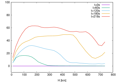
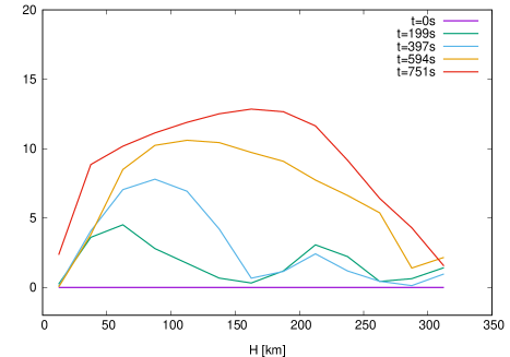
Figure 1: Time-dependent, convective velocity profiles across the accreted envelope, extracted from the 3–D simulations, and used as inputs for Models CO1 (left panel) and ONe1 (right panel).

Figure 2: Same as Fig. 1, but for the time-dependent mass dredged-up into the accreted envelope.

3 Results

As shown in Table A.1 (see Appendix A), accretion of solar composition material (Z${}_{acc}=0.02$; Model CO1) results in the pile-up of a slightly more massive envelope than for pre-enriched material (Z${}_{acc}=0.16$; Model CO2). As discussed in José et al. (2016), the single, most important nuclear reaction during the early stages of a nova outburst is ¹²C(p, $\gamma$). Its reaction rate is proportional to the product of the mass fractions of the interacting species: for Model CO1, this corresponds to 0.711 $\times$ $2.32\times 10^{-3}=1.65\times 10^{-3}$, while for Model CO2, 0.597 $\times$ $8.20\times 10^{-2}=4.90\times 10^{-2}$. Accordingly, more energy is released per second in Model CO2, that reaches a thermonuclear runaway earlier than Model CO1. This shortens the overall duration of the accretion stage in Model CO2, which in turn reduces the amount of mass accreted in this model. Thus, while Model CO1 accretes $8.39\times 10^{-5}$ M_⊙, Model CO2 accumulates $4.38\times 10^{-5}$ M_⊙ (however, since 16% of the accreted material in Model CO2 corresponds to white dwarf material, the net amount of new material piled up on top of the star accounts for only $3.68\times 10^{-5}$ M_⊙).

As discussed by Shara (1981) and Fujimoto (1982), the strength of a nova outburst is determined by the pressure achieved at the core-envelope interface, P_ce, a measure of the overall pressure exerted by the mass overlying the ignition shell,

$$P_{ce}=\frac{GM_{wd}}{4\pi R_{wd}^{4}}\Delta M_{acc}$$ (6)

where G is the gravitational constant, M_wd and R_wd the mass and radius of the white dwarf that hosts the explosion, and $\Delta M_{acc}$ the mass of the accreted envelope. Mass ejection from the white dwarf surface is achieved for pressures around P${}_{ce}\sim 10^{19}$ - $\sim 10^{20}$ dyn cm^-2 (Fujimoto 1982, MacDonald 1983). Because of the relationship between stellar radius and mass, Eq. 6 shows that, for a given white dwarf mass, $P_{ce}$ depends only on the mass of the accreted envelope. Mass accretion onto these CO-rich white dwarfs yields maximum $P_{ce}$ of $1.77\times 10^{19}$ dyn cm^-2 (Model CO1) and $9.49\times 10^{18}$ dyn cm^-2 (Model CO2). Thus, more violent outbursts, characterized by higher peak temperatures, T_max, are expected for Model CO1, since it accumulates about twice as much mass as Model CO2. Indeed, Model CO1 achieves T${}_{max}=1.92\times 10^{8}$ K, while Model CO2 reaches only T${}_{max}=1.72\times 10^{8}$ K.

The greater amount of mass accreted in Model CO1 translates into a greater ejected mass, $\Delta M_{eje}=8.33\times 10^{-5}$ M_⊙, with a mean kinetic energy of $1.17\times 10^{45}$ ergs. In contrast, Model CO2 ejects $\Delta M_{eje}=3.54\times 10^{-5}$ M_⊙, with a mean kinetic energy of $5.28\times 10^{44}$ ergs. A mean metallicity of Z${}_{eje}=0.16$ in the ejecta is obtained in Model CO1, mostly as a result of dredge-up from the outermost white dwarf layers. In terms of nucleosynthesis, differences in chemical abundances between Models CO1 and CO2 are within a factor of 2 for most species. Notable exceptions include the light elements ³He and ⁷Be (⁷Li). Their time-evolution is strongly influenced by the longer duration of the accretion phase in Model CO1. ⁷Be, in particular, is a very fragile species. It is synthesized during the early stages of the runaway by ³He($\alpha$, $\gamma$)⁷Be, and efficiently destroyed by proton-capture reactions, ⁷Be(p, $\gamma$)⁸B. However, photodisintegration reactions on ⁸B become important at temperatures above $\geq 10^{8}$ K, such that a quasi-equilibrium between the (p, $\gamma$) and the ($\gamma$, p) channels is established, preserving the amount of ⁷Be at this stage (Hernanz et al. 1996, José & Hernanz 1998). Therefore, the final amount of ⁷Be in the ejecta, that transforms into ⁷Li by electron captures, critically depends on the amount available before quasi-equilibrium is reached. This, in turn, depends on the characteristic timescale of the early runaway: the greater the product X(¹H) X(¹²C), the faster the thermonuclear runaway develops and the larger the amount of ⁷Li in the ejecta. Accordingly, and as expected, the new 123-321 nova models result in a net reduction of the ⁷Li produced by novae. Other differences are found in the Mg-Al mass region, where the abundance of ^26gAl, in particular, is decreased by a factor of $3$ in Model CO1 with respect to the pre-enriched Model CO2.

Regarding ONe models, differences in the overall accreted masses are much smaller than for CO models. This is due to similar values of the product X(¹H) $\times$ X(¹²C): $1.65\times 10^{-3}$, as before, for accretion of solar material (Model ONe1), and 0.548 $\times$ $3.90\times 10^{-3}$ = $2.14\times 10^{-3}$ for the pre-enriched Model ONe2. As noted above, the greater the value of the product X(¹H) $\times$ X(¹²C), the lower the mass accumulated in the envelope before the thermonuclear runaway sets in. Model ONe1 accretes $2.29\times 10^{-5}$ M_⊙, while Model ONe2 accretes $2.12\times 10^{-5}$ M_⊙ of pre-enriched material (out of which, $1.63\times 10^{-5}$ M_⊙ was transferred from the stellar companion). Maximum temperatures and pressures achieved at the core-envelope interface also reflect the similar masses accreted: T${}_{max}=2.40\times 10^{8}$ K and P${}_{ce}=2.77\times 10^{19}$ dyn cm^-2, for Model ONe1; T${}_{max}=2.38\times 10^{8}$ K and P${}_{ce}=2.59\times 10^{19}$ dyn cm^-2, for Model ONe2. As found for the CO models, greater ejected masses with higher kinetic energies were also obtained in the new ONe model with solar accretion and dredge-up: $2.65\times 10^{-5}$ M_⊙ and $1.09\times 10^{45}$ ergs for Model ONe1, while $1.71\times 10^{-5}$ M_⊙ and $0.99\times 10^{45}$ ergs for Model ONe2. A mean, mass-averaged metallicity in the ejecta of Z${}_{eje}=0.23$ was obtained in Model ONe1. The larger temperatures achieved by the ONe Models extend their nuclear activity up to Ca. Differences in yields between Models ONe1 and ONe2 reach a factor of $\sim 3$ for many intermediate-mass elements. Most notably, ⁷Be (⁷Li) is reduced by a factor $54$ in the new models with dredge-up (i.e., Model ONe1). The mean mass fraction of the $\gamma$-ray emitter ²²Na decreases by a factor of $\sim 2$ in Model ONe1 compared with the value obtained in Model ONe2, while no notable variation is found for ²⁶Al. Other nuclear species, such as ¹⁶O, ²¹Ne, ²³Na and ^24,26Mg, present abundance variations by factors ranging between $8$ and $290$, up and down, when yields from Model ONe1 are compared to values obtained for the pre-enriched Model ONe2 (see Table A.1 and Figs. 3 and 4).

Figure 3: Mean overproduction factors, relative to solar (Lodders 2009), in the ejecta of Models CO1 (left panel) and CO2 (right panel). In the plots, unstable nuclei (e.g., ⁷Be) have been assumed to decay into the corresponding stable species (e.g., ⁷Li).

Figure 4: Same as Fig. 3, for Models ONe1 (left panel) and ONe2 (right panel).

4 Discussion and Conclusions

This work reports on a new methodology applied to the modeling of nova outbursts, through the use of 1–D and 3–D simulations. It explores, for the first time, the combined effect of mass dredge-up and the inverse energy cascade that characterizes 3–D turbulent convection on the characteristics of the explosion.

More massive envelopes than those reported from previous models with pre-enrichment have been obtained, providing better agreement with spectroscopically inferred masses. The lower estimates systematically predicted by hydrodynamic simulations until now have been regarded as a major drawback of the thermonuclear nova model (see, however, Shore et al. 2016, Mason et al. 2018, for studies of ejected masses based on reanalyses of filling factors). The greater pressures achieved at the envelope base power, in turn, more violent outbursts, characterized by higher peak temperatures and greater ejected masses, with metallicity enhancements in agreement with observations. As shown in Fig. 5, the convective velocities based on our 3–D simulations exhibit smoother profiles than those based on mixing-length theory (for $\alpha$ = 1). The latter yields more erratic convective patterns, in which convective regions are separated by purely radiative layers. Moreover, maximum convective velocities obtained in our 3–D simulations exceed the estimates based on mixing-length theory when convective transport almost extends through the entire envelope (i.e., at 120 s and 218 s). Such convective velocites are distinctly subsonic, as can be shown by comparison with the values of the local speed of sound, $c_{s}$, calculated as:

$$c_{s}=\sqrt{\left(\frac{\partial P}{\partial\rho}\right)_{\rm S}}=\sqrt{\left(\frac{\partial P}{\partial\rho}\right)_{\rm T}+\frac{T}{\rho^{2}}\frac{\left(\frac{\partial P}{\partial T}\right)^{2}_{\rm\rho}}{\left(\frac{\partial U}{\partial T}\right)_{\rm\rho}}}$$ (7)

where $S$ is the entropy and $U$ is the internal energy per unit mass.

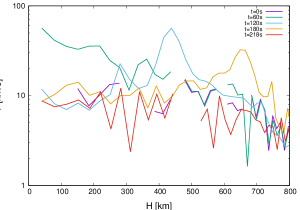
Figure 5: Convective velocity (derived from mixing-length theory for $\alpha=1$) as function of depth, for the same times displayed in Fig. 1 (left panel; Model CO1).

Due to the Eulerian nature of the FLASH code, our 3–D simulations must be stopped when the convective front hits the upper boundary of the computational domain. This limits the extent of the multidimensional simulations, that cannot proceed through most of the expansion and ejection stages. Therefore, prescriptions for the time-dependent amount of mass dredged-up and convective velocity are not available much beyond the peak of the explosions. To overcome this limitation, in the 321 simulations reported in this work, mass dredge-up is extrapolated from the last data points available from the 3–D simulations. With regard to the time-dependent convective velocity, no extrapolation is made. Instead, SHIVA switches to a time-dependent mixing length prescription at longer times, to properly account for the progressive retreat of convection from the outermost envelope layers. It is worth noting that the general trends reported in this paper (i.e., larger accreted and ejected masses, favoring a better agreement with the values inferred spectroscopically; more violent outbursts, characterized by larger peak temperatures and kinetic energies; a reduction of the overall amount of ⁷Be (⁷Li) in the ejecta) are not affected by the extrapolation of the time-dependent mass dredged-up into the envelope adopted during the last stages of the outburst. However, some specific details, such as the exact amount of mass ejected in the outburst, or the final mass fractions of some nuclear species in the ejecta (particularly those dredged-up from the outermost white dwarf layers) would be affected, to some extent, by the way the mass dredged-up proceeds during the last stages of the explosion. It is also important to stress that the last stages of the outburst are characteried by decaying turbulence, and therefore mixing should persist after the explosion. Efforts aimed at extending the computational domains used in our 3–D simulations are currently underway. These should allow FLASH to proceed further, until the envelope becomes physically detached from the rest of the star, and dredge-up of white dwarf material and convection are naturally halted.

Finally, the simulations reported in this work suggest that the white dwarf mass decreases after a nova outburst, whenever metallicity enhancements in the ejecta exceed a threshold value around $Z_{eje}\sim 0.2$. This has implications for the long-debated role of classical novae as possible type Ia supernova progenitors, since the metallicities inferred from the nova ejecta frequently exceed that threshold.

Acknowledgements. The authors would like to thank Margarita Hernanz, Christian Iliadis, Giovanni Leidi, and Sumner Starrfield for fruitful discussions. This work has been partially supported by the Spanish MINECO grant AYA2017–86274–P, by the E.U. FEDER funds, and by the AGAUR/Generalitat de Catalunya grant SGR-661/2017. This article benefited from discussions within the “ChETEC” COST Action (CA16117).

Appendix A Nucleosynthesis

Table 1: Nova models computed in this work.

Model	CO1	CO2	ONe1	ONe2
Type	123-321	1–D with pre-enrichment	123-321	1–D with pre-enrichment
MWD($M_{\odot}$)	1.0	1.0	1.25	1.25
Zacc	Solar	16% CO, 84% Solar	Solar	23% ONe, 77% Solar
$\Delta$Macc($10^{-5}$ M⊙)	8.39	3.68a	2.29	1.63a
Tmax($10^{8}$ K)	1.92	1.72	2.40	2.38
K($10^{45}$ ergs)	1.17	0.528	1.09	0.99
v(km s-1)	1190	1240	2030	2410
$\Delta$Meje($10^{-5}$ M⊙)	8.33	3.54	2.65	1.71
Zeje	0.16	0.18	0.23	0.23
X(1H)	5.7(-1)	5.7(-1)	4.9(-1)	4.9(-1)
X(3He)	1.4(-9)	3.2(-6)	-	1.2(-9)
X(4He)	2.7(-1)	2.5(-1)	2.8(-1)	2.8(-1)
X(7Li)	-	1.3(-9)	-	-
X(7Be)	2.7(-9)	1.8(-6)	2.4(-9)	1.3(-7)
X(12C)	1.4(-2)	1.4(-2)	1.5(-2)	2.0(-2)
X(13C)	2.0(-2)	2.4(-2)	1.3(-2)	1.7(-2)
X(14N)	3.5(-2)	6.0(-2)	2.6(-2)	3.1(-2)
X(15N)	7.7(-3)	4.7(-3)	2.1(-2)	3.1(-2)
X(16O)	7.7(-2)	7.2(-2)	9.1(-2)	7.2(-3)
X(17O)	3.1(-3)	1.6(-3)	3.4(-3)	6.1(-3)
X(18O)b	3.4(-7)	2.5(-7)	3.8(-7)	8.9(-7)
X(18F)b	1.2(-6)	8.2(-7)	1.0(-6)	2.1(-6)
X(19F)	3.3(-9)	3.9(-9)	1.0(-8)	2.9(-8)
X(20Ne)	1.5(-3)	1.4(-3)	3.9(-2)	8.1(-2)
X(21Ne)	2.2(-7)	1.4(-7)	2.3(-4)	1.8(-5)
X(22Ne)	4.4(-5)	1.1(-4)	2.8(-4)	1.3(-4)
X(22Na)	8.5(-7)	7.3(-7)	3.2(-5)	6.5(-5)
X(23Na)	3.8(-6)	5.3(-6)	2.9(-3)	3.5(-4)
X(24Mg)	4.9(-7)	6.8(-6)	2.1(-3)	7.3(-6)
X(25Mg)	7.2(-5)	4.2(-4)	2.1(-3)	5.5(-4)
X(26Mg)	5.6(-6)	4.2(-5)	5.1(-4)	2.7(-5)
X(26gAl)	1.4(-5)	4.1(-5)	1.8(-4)	1.4(-4)
X(27Al)	1.1(-4)	1.2(-4)	1.2(-3)	9.2(-4)
X(28Si)	1.1(-3)	6.2(-4)	7.3(-3)	2.7(-2)
X(29Si)	2.0(-5)	3.0(-5)	1.5(-4)	5.5(-4)
X(30Si)	4.3(-5)	2.3(-5)	1.6(-3)	4.2(-3)
X(31P)	6.5(-6)	5.8(-6)	6.0(-4)	1.3(-3)
X(32S)	3.0(-4)	2.9(-4)	1.5(-3)	1.3(-3)
X(33S)	2.3(-6)	2.4(-6)	2.2(-6)	2.0(-6)
X(34S)	1.3(-5)	1.4(-5)	5.0(-6)	7.7(-6)
X(35Cl)	4.0(-6)	3.2(-6)	1.1(-5)	8.3(-6)
X(36Ar)	6.2(-5)	6.4(-5)	1.3(-5)	2.6(-5)
X(37Cl)	4.7(-6)	1.2(-6)	4.7(-5)	3.4(-5)
X(38Ar)	1.3(-5)	1.2(-5)	1.4(-5)	1.2(-5)
X(39K)	3.2(-6)	3.1(-6)	4.2(-6)	3.5(-6)
X(40Ca)	5.4(-5)	5.4(-5)	4.9(-5)	4.9(-5)

• Fraction of the accreted mass that corresponds to solar composition (84% and 77%, respectively), excluding pre-enrichment with white dwarf material.

• Mass fractions correspond to t = 1 hr after T_max.

References

- (1) Alexakis, A., Calder, A. C., Heger, A., et al. 2004, ApJ, 602, 931
- (2) Arnett, W. D., Meakin, C., Viallet, M., et al. 2015, ApJ, 809, 30
- (3) Biermann, L. 1932, Z. Astrophys., 5, 117
- (4) Cameron, A. G. W. 1959, ApJ, 130, 916
- (5) Casanova, J., José, J., García–Berro, E., Calder, A., & Shore, S. N. 2010, A&A, 513, L5
- (6) Casanova, J., José, J., García–Berro, E., Calder, A., & Shore, S. N. 2011a, A&A, 527, A5
- (7) Casanova, J., José, J., García–Berro, E., Shore, S. N., & Calder, A. C. 2011b, Nature, 478, 490
- (8) Casanova, J., José, J., García–Berro, E., & Shore, S. N. 2016, A&A, 595, A28
- (9) Casanova, J., José, J., & Shore, S. N. 2018, A&A, 619, A121
- (10) Denissenkov, P. A., Herwig, F., Bildsten, L., & Paxton, B. 2013, ApJ, 762, 8
- (11) Diaz, M. P., & Bruch, A. 1997, A&A , 322, 807
- (12) Durisen, R. H. 1977, ApJ, 213, 145
- (13) Fujimoto, M. Y. 1982, ApJ, 257, 752
- (14) Fujimoto, M. Y. 1988, A&A, 198, 163
- (15) Fujimoto, M., & Iben, I., Jr. 1992, ApJ, 399, 646
- (16) Giannone, P., & Weigert, A. 1967, Z. Astrophys., 67, 41
- (17) Glasner, S. A., & Livne, E. 1995, ApJ, 445, L149
- (18) Glasner, S. A., Livne, E., & Truran, J. W. 1997, ApJ, 475, 754
- (19) Glasner, S. A., Livne, E., & Truran, J. W. 2005, ApJ, 625, 347
- (20) Glasner, S. A., Livne, E., & Truran, J. W. 2007, ApJ, 665, 1321
- (21) Glasner, S. A., Livne, E., & Truran, J. W. 2012, MNRAS, 427, 2411
- (22) Gurevitch, L. E., & Lebedinsky, A. I., 1957, in Non-Stable Stars, eds. G. H. Herbig (Cambridge, UK: Cambridge Univ. Press), 77
- (23) Hernanz, M., José, J., Coc, A. & Isern, J. 1996, ApJ, 465, L27
- (24) Hillman, Y., Prialnik, D., Kovetz, A., & Shara, M. M. 2016, ApJ, 819, 168
- (25) Iben, I., Jr., Fujimoto, M. Y., & MacDonald, J. 1991, ApJ, 375, L27
- (26) Iben, I., Jr., Fujimoto, M. Y., & MacDonald, J. 1992, ApJ, 388, 521
- (27) José, J. 2016, Stellar Explosions: Hydrodynamics and Nucleosynthesis (Boca Raton, FL: CRC/Taylor and Francis)
- (28) José, J., Halabi, G. M., & El Eid, M. F. 2016, A&A, 593, A54
- (29) José, J. & Hernanz, M. 1998, ApJ, 494, 680
- (30) José, J., & Shore, S. 2008, in Classical Novae, 2nd edn., eds. M. F. Bode, & A. Evans (Cambridge, UK: Cambridge Univ. Press), 121
- (31) Kippenhahn, R., & Thomas, H. 1978, A&A, 63, 265
- (32) Kovetz, A., & Prialnik, D. 1985, ApJ, 291, 812
- (33) Kutter, G. S., & Sparks, W. M. 1987, ApJ, 321, 386
- (34) Kutter, G. S., & Sparks, W. M. 1989, ApJ, 340, 985
- (35) Leidi, G., 2019, MSc Thesis (Univ. Pisa, Italy)
- (36) Leidi, G., Shore, S. N., & José, J., 2019, in preparation
- (37) Lesieur, M., Yaglom, A., & David, F. (eds.) 2001, New Trends in Turbulence, Les Houches 2000 Summer School, vol. 74 (Berlin: Springer-Verlag)
- (38) Livio, M., & Truran, J. W. 1987, ApJ, 318, 316
- (39) Livio, M., & Truran, J. W. 1990, in Proc. 5th Florida Workshop in Nonlinear Astronomy, 617, 126
- (40) Lodders, K., Palme, H., & Gail, H.-P. 2009, in Solar System, ed. J. E. Trümper, Landolt-Börnstein New Series VI/4B (Berlin: Springer-Verlag)
- (41) MacDonald, J. 1983, ApJ, 273, 289
- (42) Martin, D., Longland, R., & José, J. 2018, CompAC, 5, 3
- (43) Mason, E., Shore, S. N., De Gennaro Aquino, I., et al. 2018, ApJ, 853, 27
- (44) Pope, S.B. 2000, Turbulent Flows (Cambridge Univ. Press: Cambridge)
- (45) Prialnik, D., Shara, M. M., & Shaviv, G. 1978, A&A, 62, 339
- (46) Prialnik, D., Shara, M. M., & Shaviv, G. 1979, A&A, 72, 192
- (47) Prialnik, D., & Kovetz, A. 1984, ApJ, 281, 367
- (48) Richtmyer, R. D., & Morton, K. W. 1994, Difference Methods for Initial-Value Problems, 2nd edn. (Krieger Publishing Co.: Malabar, FL)
- (49) Rose, W. K. 1968, ApJ, 152, 245
- (50) Rosner, R., Alexakis, A., Young, Y., Truran, J. W., & Hillebrandt, W. 2001, ApJ, 562, L177
- (51) Rukeya, R., Lü, G., Wang, Z., & Zhu C. 2017, PASP, 129, 074201
- (52) Schatzman, E. 1949, Ann. Astrophys., 12, 281
- (53) Schatzman, E. 1951, Ann. Astrophys., 14, 294
- (54) Shafter, A. W. 2017, ApJ, 834, 196
- (55) Shara, M. M. 1981, ApJ, 243, 926
- (56) Shore, S. N., Mason, E., Schwarz, G. J., et al. 2016, ApJ, 590, A123
- (57) Sparks, W. M. 1969, ApJ, 156, 569
- (58) Sparks, W. M., & Kutter, G. S. 1987, ApJ, 321, 394
- (59) Starrfield, S. 1971a, MNRAS, 152, 307
- (60) Starrfield, S. 1971b, MNRAS, 155, 129
- (61) Starrfield, S., Iliadis, C., & Hix, W. R. 2008, in Classical Novae, 2nd edn., eds. M. F. Bode, & A. Evans (Cambridge, UK: Cambridge Univ. Press), 77
- (62) Starrfield, S., Iliadis, C., Timmes, F. X., et al. 2012, BASI, 40, 419
- (63) Starrfield, S., Iliadis, C., & Hix, W. R. 2016, PASP, 128, 051001
- (64) Starrfield, S., Truran, J. W., Sparks, W. M., & Kutter, G.S. 1972, ApJ, 176, 169
- (65) Starrfield, S., Truran, J. W., Wiescher, M. C., & Sparks, W. M. 1998, MNRAS, 296, 502
- (66) Wood, P. R. 1974, ApJ, 190, 609
- (67) Woosley, S. E. 1986, in Nucleosynthesis and Chemical Evolution, eds. B. Hauck, A. Maeder, & G. Meynet (Geneva Observatory: Sauverny), 1
- (68) Yaron, O., Prialnik, D., Shara, M. M., & Kovetz, A. 2005, ApJ, 623, 398