Inverse Compton scattering from solid targets irradiated by ultra-short laser pulses in the ${10}^{22}\text{\,}$ – ${10}^{23}\text{\,}\mathrm{W}\mathrm{/}\mathrm{c}\mathrm{m}^{2}$ regime

Abstract

Emission of high energy gamma rays via the non-linear inverse Compton scattering process (ICS) in interactions of ultra-intense laser pulses with thin solid foils is studied using particle-in-cell simulations. It is shown that the angular distribution of the ICS photons has a forward-oriented two-directional structure centred at an angle $\vartheta=\pm$$$, a value predicted by a theoretical model based on a standing wave approximation to the electromagnetic field in front of the target, which only increases at the highest intensities due to faster hole boring, which renders the approximation invalid. The conversion efficiency is shown to exhibit a super-linear increase with the driving pulse intensity. In comparison to emission via electron-nucleus bremsstrahlung, it is shown that the higher absorption, further enhanced by faster hole boring, in the targets with lower atomic number strongly favours the ICS process.

Keywords laser plasma, inverse Compton scattering, gamma rays, radiation reaction, foil targets, particle-in-cell

1 Introduction

Next generation high-power laser systems are expected to routinely reach intensities in the $I\approx${10}^{22}$-${10}^{23}\text{\,}\mathrm{W}\mathrm{/}\mathrm{c}\mathrm{m}^{2}$$ region [1, 2, 3, 4]. In a configuration where such an intense pulse interacts with a solid target, gamma rays will be generated mostly by the processes of electron-nucleus bremsstrahlung [5], and by radiation reaction effects including non-linear inverse Compton scattering (ICS) [6, 7], where the fast electrons scatter on the high field of the laser pulse itself [8]. In this paper, we present a study of the latter process, relevant especially at the higher end of the considered intensity range, where the radiation has to be treated in the context of quantum electrodynamics (QED), with the further outlook of even higher intensities which would exhibit additional important effects such as the creation of electron-positron pairs and QED cascades [9, 10, 11, 12, 13, 14, 15, 16].

The non-linear multi-photon nature of the ICS process requires the presence of fast electrons and high fields. In the context of laser-plasma interactions, it has been observed in various configurations where the laser pulse interacts with an accelerated electron beam. Early observations [17, 18, 19, 20, 21, 22] of multi-photon scattering on fast electrons were limited to the regime of low energy of the emitted photons, $\hbar\omega_{\gamma}\ll m_{\textup{e}}c^{2}$, where $\hbar$ is the reduced Planck constant, $\omega_{\gamma}$ the photon’s angular frequency, $m_{\textup{e}}$ the electron mass, and $c$ the speed of light, which is commonly called non-linear Thomson scattering as opposed to (non-linear) inverse Compton scattering where $\hbar\omega_{\gamma}\gg m_{\textup{e}}c^{2}$ [7]. These were followed by observations of the ICS interaction in the non-quantum regime in experiments with laser wakefield accelerated electrons and a counter-propagating laser pulse with the gamma ray energies of $\mathcal{E}_{\gamma}=6-$18\text{\,}\mathrm{M}\mathrm{e}\mathrm{V}$$ [23], and $\mathcal{E}_{\gamma}>$20\text{\,}\mathrm{M}\mathrm{e}\mathrm{V}$$ [24], though the authors stick to calling the interaction the non-linear Thomson process in order to highlight that the quantum effects are still negligible in this regime. The energies high enough to probe the quantum nature of the interaction, as opposed to the classical radiation reaction approximation, were not reached until 2018 when a landmark experiment by Cole et al. [25], performed at the Astra Gemini laser, presented evidence of radiation reaction in the collision of an ultra-relativistic $\mathcal{E}_{\textup{e}}>$500\text{\,}\mathrm{M}\mathrm{e}\mathrm{V}$$ electron beam generated by laser-wakefield acceleration with an intense $I=$1.3\text{\times}{10}^{21}\text{\,}\mathrm{W}\mathrm{/}\mathrm{c}\mathrm{m}^{2}$,a_{0}=25$ laser pulse. The energy loss in the post-collision electron spectrum was correlated with the detected $\mathcal{E}_{\gamma}>$30\text{\,}\mathrm{M}\mathrm{e}\mathrm{V}$$ gamma ray signal, and was found to be consistent with a quantum description of radiation reaction. A further experiment [26] with a $I=$4\text{\times}{10}^{20}\text{\,}\mathrm{W}\mathrm{/}\mathrm{c}\mathrm{m}^{2}$$ pulse provided additional signatures of quantum effects in the electron dynamics in the external laser field, potentially showing departures from the constant cross field approximation.

Unlike the experiments where an intense laser pulse interacts with a solitary electron beam, the hot electrons participating in ICS in the laser-solid interactions studied in this paper are self-generated at the front side of the target due to the absorption [27, 28] of a portion of the energy of the same pulse with which they immediately interact giving out high-energy gamma rays. By means of Particle-in-Cell simulations using the code EPOCH [29], we study the ICS emission from thin foils as a function of the laser pulse intensity, describe its energy spectrum and angular distribution, and present a simplified standing-wave model that explains some of the emission’s prominent features. Additionally, we examine the effect of target material, and compare the ICS emission to bremsstrahlung, which we studied in our previous paper [30] under the same conditions.

The paper is organized as follows. Section 2 summarizes the essential theoretical background, and section 3 describes the PIC simulation setup. Section 4 presents the results, in particular the simulated ICS photon energy spectra, the simplified standing wave model and its comparison to the PIC simulations, the description of electron dynamics at the front side of the target, the predicted emission angle of the ICS photons and the angular distribution obtained from the PIC simulations, the efficiency of conversion of the driving laser pulse energy into that of the ICS photons, and a comparison of ICS to bremsstrahlung emission. Section 5 summarizes our conclusions.

2 Gamma ray emission by inverse Compton scattering

The ICS radiation is in fact not emitted continuously. Individual photons are emitted as the electron loses energy due to its interaction with the strong field. To characterize this interaction, taking into account the discontinuous nature of the process, a parameter $\chi_{\textup{e}}$ is introduced [6, 11, 31]:

$$\chi_{\textup{e}}=\frac{1}{E_{\textup{S}}}\sqrt{\left(\gamma\mathbf{E}+\frac{\mathbf{p}\times\mathbf{B}}{m_{\textup{e}}}\right)^{2}-\left(\frac{\mathbf{p}\cdot\mathbf{E}}{m_{\textup{e}}c}\right)^{2}}\\$$ (1)

where $\mathbf{E}$ is the electric field, $\mathbf{B}$ is the magnetic field, $\mathbf{p}$ is the electron momentum, $\gamma=1/\sqrt{1-v^{2}/c^{2}}$ is the relativistic Lorentz factor of the electron, and $E_{\textup{S}}$ is the “Sauter-Schwinger” field [32, 33], a critical field with enough strength to be able to perform $m_{\textup{e}}c^{2}$ work over the electron Compton length $\lambdabar_{\textup{C}}=\hbar/m_{\textup{e}}c$ [11], $E_{\textup{S}}=m_{\textup{e}}^{2}c^{3}/e\hbar=$1.32\text{\times}{10}^{16}\text{\,}\mathrm{V}\mathrm{/}\mathrm{c}\mathrm{m}$$. Regarding the emission of gamma rays, the value of $\chi_{\textup{e}}$ indicates the strength of the radiation process, roughly separating the classical regime $\chi_{\textup{e}}\ll 1$ with continuous emission, and the quantum regime, where $\chi_{\textup{e}}$ approaches unity and the process must be treated as a discontinuous emission of photon quanta [34, 13].

The intensity of the gamma radiation emitted by the electron can be expressed in the limits of $\chi_{\textup{e}}\ll 1$ or $\chi_{\textup{e}}\gg 1$ respectively as

$$I_{\textup{rad}}^{<} =\frac{e^{2}m_{\textup{e}}^{2}}{6\pi}\chi_{\textup{e}}^{2}(1-c_{1}\chi_{\textup{e}}+c_{2}\chi_{\textup{e}}^{2}-\ldots),$$ (2a)

$$I_{\textup{rad}}^{>} =c_{3}\frac{e^{2}m_{\textup{e}}^{2}}{6\pi}\chi_{\textup{e}}^{2/3}(1-c_{4}\chi_{\textup{e}}^{-2/3}+c_{5}\chi_{\textup{e}}^{-4/3}-\ldots)$$ (2b)

where $e$ is the elementary charge, and $c_{1},\ldots,c_{5}$ are constants [35]. We can then give a rough estimate of the extreme limits for radiation intensity. At very small $\chi_{\textup{e}}$, we can only keep the unit term in the brackets of equation (2a), and the radiation intensity behaves as $I_{\textup{rad}}\sim\chi_{\textup{e}}^{2}$, while at very large $\chi_{\textup{e}}$, those terms in the brackets of equation (2b) which are inversely proportional to $\chi_{\textup{e}}$ raised to some positive power can be neglected, and the radiation intensity then behaves as $I_{\textup{rad}}\sim\chi_{\textup{e}}^{2/3}$.

Previous equations show that in order to generate large amounts of high energy gamma rays, one needs to employ a high field, hot electrons, or both. The strength of the laser pulse can be expressed in terms of the normalized amplitude of the vector potential

$$a_{0}=\frac{eE_{0}}{m_{\textup{e}}\omega c}\approx(7.3\times 10^{-19}(\lambda[$\mathrm{\SIUnitSymbolMicro m}$])^{2}I[$\mathrm{W}\,\mathrm{c}\mathrm{m}^{-2}$])^{1/2},$$ (2c)

where $E_{0}$ is the peak amplitude of the electric field of the laser pulse, $\omega$ its angular frequency, and $\lambda$ its wavelength. The temperature of the hot electrons pulled out of a solid target by a pulse in the non-linear relativistic regime is given by

$$T_{\textup{e}}=m_{\textup{e}}c^{2}(\gamma-1),$$ (2d)

the relativistic $\gamma$ factor can be, in laser-solid interactions, approximated from the ponderomotive scaling [36] in the case of linear polarization as

$$\gamma=\sqrt{1+\frac{a_{0}^{2}}{2}},$$ (2e)

For high values of $a_{0}$, this leads to a linear dependence $T_{\textup{e}}\sim a_{0}$.

3 Simulation setup

Simulations were done in 2D in a $x\in(-15,15)\;$\mathrm{\SIUnitSymbolMicro m}$$, and $y\in(-20,20)\;$\mathrm{\SIUnitSymbolMicro m}$$ box with a cell size of $10\times$10\text{\,}\mathrm{n}\mathrm{m}$$. A normally incident laser pulse polarized in the simulation plane with a wavelength $\lambda=$1\text{\,}\mathrm{\SIUnitSymbolMicro m}$$, and a Gaussian spatial and temporal profile with a FWHM duration of $\tau=$30\text{\,}\mathrm{f}\mathrm{s}$$, was propagating along the $x$ axis, and focused to a $w=$3\text{\,}\mathrm{\SIUnitSymbolMicro m}$$ spot at the front side of the target placed at $x=0$. The laser pulse was emitted from the $x=$-15\text{\,}\mathrm{\SIUnitSymbolMicro m}$$ boundary at the start of the simulation $t=0$, at an angle of $\vartheta_{\mathrm{L}}=$$$ with its peak intensity crossing the boundary at $t=$60\text{\,}\mathrm{f}\mathrm{s}$$. The target was composed of a fully ionized CH plasma with electron density $n_{\textup{e}}=289n_{\textup{c}}$, where $n_{\textup{c}}=\epsilon_{0}m_{\textup{e}}\omega^{2}/e^{2}$ is the plasma critical density which is a function of the angular frequency $\omega$ of the laser pulse, with $\epsilon_{0}$ being the permittivity of free space. For a $\lambda=$1\text{\,}\mathrm{\SIUnitSymbolMicro m}$$ laser pulse, the value of $n_{\textup{c}}=$1.1\text{\times}{10}^{21}\text{\,}\mathrm{c}\mathrm{m}^{-3}$$. Parameter scans were performed for six laser pulse intensities between $I=$3\text{\times}{10}^{21}\text{\,}\mathrm{W}\mathrm{/}\mathrm{c}\mathrm{m}^{2}$$, and $I=${10}^{23}\text{\,}\mathrm{W}\mathrm{/}\mathrm{c}\mathrm{m}^{2}$$. The normalized potential corresponding to the intensities in the simulations ranges from $a_{0}=47$ to $a_{0}=270$. Two additional materials, Al, and Au, were examined in order to compare these results to our previous work [30], which also describes their respective simulated parameters.

The simulations used a second order FDTD Maxwell solver [37], and a relativistic Boris pusher [38]. To limit noise and numerical heating [29], the simulations included a current smoothing algorithm and third order particle weighting. All boundary conditions were absorbing for radiation and thermalizing for particles. The radiation reaction effects were calculated EPOCH’s Monte Carlo algorithm [39], and bremsstrahlung [30] was taken into account in order to obtain a self-consistent results. This paper only uses the photons with $\mathcal{E}_{\gamma}>$1\text{\,}\mathrm{M}\mathrm{e}\mathrm{V}$$ in all subsequent analysis.

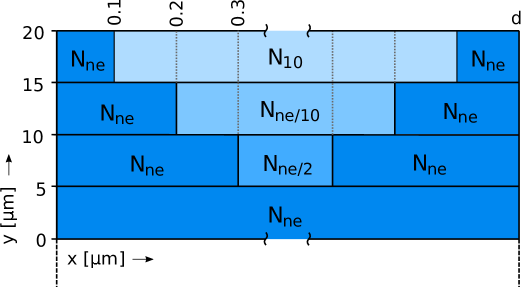
Figure 1: Schematic representation of the splitting of the simulated target with the width $d$ into regions containing different number of computational macro-particles per cell. The figure only shows the top half $y>0$ of the target, with the bottom half being symmetric with respect to the $x$ axis. The axes in the figure are not to scale.

Table 1: Number of macro-particles in different regions of the simulated target. The first column lists the designation $N_{\mathrm{ppc}}$ of a computational region, which is equal to the number of electron macro-particles per cell in that region. The second column lists the value of $N_{\mathrm{ppc}}$, i.e. the number of macro-particles per cell. The third column lists the number of ion macro-particles per cell either as an absolute value, or with respect to the number of electron macro-particles. The fourth column gives the extent of the given region along the $y$ axis, and the last column shows the width of the “guard region”, composed of cells with the full number of macro-particles, at both ends of the $x$ axis of the main region, where applicable.

region	number of	number of	transverse	guard
	electrons	ions	extent [$\mathrm{\SIUnitSymbolMicro m}$]	width [$\mathrm{\SIUnitSymbolMicro m}$]
$N_{n_{e}}$	$n_{e}/n_{c}$	$N_{n_{e}}/Z$	$(\phantom{0}0,\phantom{0}5)$	–
$N_{n_{e}/2}$	$N_{n_{e}}/2$	$N_{n_{e}/2}/Z$	$(\phantom{0}5,10)$	0.3
$N_{n_{e}/10}$	$N_{n_{e}}/10$	$N_{n_{e}/10}/Z$	$(10,15)$	0.2
$N_{10}$	$10$	$2$	$(15,20)$	0.1

The number of macro-particles varied along the y axis to ensure adequate resolution with $N_{n_{e}}=n_{e}/n_{c}$ electron macro-particles per cell in the middle of the simulated target, and save computational time at its far end where the background plasma dynamics is less violent. This was achieved by dividing the target into regions, schematically depicted in figure 1, with reduced number of particles per cell $N_{\mathrm{ppc}}$ compared to the base value of $N_{n_{e}}=n_{e}/n_{c}$. To maintain the same initial electron density $n_{e}$, these particles have been given an appropriately higher computational weight. Regions with lower $N_{\mathrm{ppc}}$, summarized in table 1, were guarded with a thin layer of cells containing the base number of particles $N_{n_{e}}$ so that the simulated plasma expansion into the vacuum could represent densities lower than those represented by the higher weight particles. The target subdivision is the same as in [30] apart form the transverse extent of the target which is only $y\in(-20,20)\;$\mathrm{\SIUnitSymbolMicro m}$$ in this paper. Unless explicitly stated otherwise, we model the target as an idealized flat surface foil with no presence of pre-plasma.

4 Results

4.1 Photon spectra

Figure 2 shows the spectra of all photons generated during the simulation via the inverse Compton scattering process. The EPOCH algorithm is set up so that the minimum energy of an emitted photon is $\mathcal{E}_{\gamma}>$100\text{\,}\mathrm{k}\mathrm{e}\mathrm{V}$$, though we limit the analysis to photons with $\mathcal{E}_{\gamma}>$1\text{\,}\mathrm{M}\mathrm{e}\mathrm{V}$$. In this case, there exists a threshold laser pulse intensity $I\simeq$3\text{\times}{10}^{21}\text{\,}\mathrm{W}\mathrm{/}\mathrm{c}\mathrm{m}^{2}$$, corresponding to $a_{0}\simeq 50$ potential, below which no ICS-produced photons are seen in the simulation. The tail of this distribution can be approximated by an exponential temperature fit $N_{\gamma}\approx\exp\left(-\mathcal{E}_{\gamma}/k_{\textup{B}}T_{\gamma}\right)$, included in the figure.

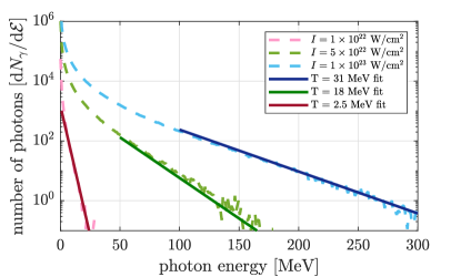
Figure 2: Spectra of photons radiated via the inverse Compton scattering process from a $d=$2\text{\,}\mathrm{\SIUnitSymbolMicro m}$$ thick CH foil at three different driving pulse intensities. The tail of each spectrum curve is overlaid with an exponential temperature fit.

Unlike the bremsstrahlung case [30], where the effective photon temperature is linear in the potential $T_{\gamma}^{\textup{BS}}\sim a_{0}\sim\sqrt{I}$, the temperature of the simulated photons emitted by the ICS process, shown in figure 3, reveals a scaling linear in the intensity

$$T_{\gamma}\sim a_{0}^{2}\sim I.$$ (2f)

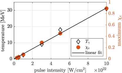
Figure 3: Effective temperature $T_{\gamma}$ of the emitted inverse Compton scattering photons, and the maximum emission parameter $\chi_{\textup{e}}$ attained by hot electrons from a $d=$2\text{\,}\mathrm{\SIUnitSymbolMicro m}$$ CH foil interacting with laser pulses of different intensities.

The $\chi_{\textup{e}}$ parameter governing the emission process depends on both the velocity of the electron and the strength of the external field $E$ to which it is subjected in a given moment,

$$\chi_{\textup{e}}\sim\gamma E\sim I.$$ (2g)

This follows from the observation that as the ponderomotive scaling equation (2d) holds, and the $\gamma$ factor attained by the hot electron population $\gamma\sim a_{0}\sim\sqrt{I}$, the emission parameter ought to be proportional to both the gamma factor and the strength of the electric field $E\sim\sqrt{I}$, thus being linearly dependent on the intensity as shown in figure 3. Though since the electron temperature is $T_{\textup{e}}\sim\sqrt{I}$, and the photon temperature must be $T_{\gamma}<T_{\textup{e}}$, there has to be a turning point where the raise in $T_{\gamma}$ slows down at some higher intensity, and the scaling $T_{\gamma}\sim I$ ceases to be valid.

An estimate for the most common energy of the resulting radiation has been proposed in the monochromatic approximation, giving $\hbar\omega_{\gamma}\simeq 0.44\chi_{\textup{e}}\gamma m_{\textup{e}}c^{2}$ [10, 31, 13]. This expression though describes the maximum of the photon distribution while the effective photon temperature $T_{\gamma}$ comes form a fit of the tail of a distribution which covers photons emitted by all of the electrons over the course of the simulation, therefore this expression cannot not predict the temperature of the photons based on that of the electrons in our situation. As the immediate value of $\chi_{\textup{e}}$ depends on the exact trajectory of the electron, a simple connection between the temperature $T_{\textup{e}}$ of the accelerated electron bunches and the temperature of the resulting radiation $T_{\gamma}$ cannot be made in the complex case of the laser-solid interaction where the bunch is of a finite size and, consequently, the different electrons interact with the field in a different phase. This is evident from the snapshot in figure 4, obtained from detailed studies of electron trajectories presented later in section 4.3, which shows the relation between the $\gamma$ factor and the $\chi_{\textup{e}}$ parameter of the simulated electrons. We observe that there are many hot electrons which have the same $\gamma$ factor but span a broad range of attained $\chi_{\textup{e}}$. Therefore, the immediate electron temperature $T_{\textup{e}}$ does not readily reveal the radiation temperature $T_{\gamma}$, though averaging over many samples during the course of the whole interaction where both the $\gamma$ factor and the field strength vary with each laser cycle would ultimately lead to a Maxwell-Boltzmann like distribution. Though we see that the maximum $\chi_{\textup{e}}$ is linear in electron energy, the linear scaling $T_{\gamma}\sim a_{0}^{2}\sim I$, which turns out quite clearly in figure 3, should be treated as an empirical observation.

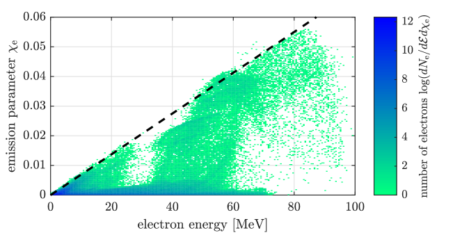
Figure 4: Emission parameter $\chi_{\textup{e}}$ plotted against the electron $\gamma$ factor from a snapshot taken at the peak emission time of a half-cycle around $t=$110\text{\,}\mathrm{f}\mathrm{s}$$ from a simulation of a $d=$2\text{\,}\mathrm{\SIUnitSymbolMicro m}$$ CH foil interacting with a $I=${10}^{22}\text{\,}\mathrm{W}\mathrm{/}\mathrm{c}\mathrm{m}^{2}$$ laser pulse (cf. figure 8 with a snapshot of the same set of electrons). The colour indicates the number of electron macro-particles of a particular energy and emission parameter in log scale.

4.2 Standing wave model

The inverse Compton scattering process involves an electron moving in the field of the laser pulse in front of the target. To obtain more insight into the physical mechanisms governing the emission, we will make use of the simulation data with high temporal resolution with the help of a simplified theoretical model derived to describe the electron motion based on the standing wave approximation, which will be solved numerically.

As the electromagnetic wave of the linearly polarized laser pulse impinges on the highly overdense flat plasma slab at $x=0$, most of it is reflected back and interferes with the incoming part of the pulse forming a standing wave in front of the target. The more equal the incident and reflected pulses, the more pronounced the standing wave pattern. In the case of a very short pulse, where the field intensity of the envelope changes rapidly with each oscillation, this pattern would be most prominent around the peak of the laser-target interaction where the intensity profile of the incoming and the reflected waves are approximately equal. The electric and magnetic field of the standing wave formed in front of the target in the case of normal incidence can be approximated by a plane wave near the interaction centre, and characterized by:

$$\eqalign{E_{\textup{y}}=E_{0}\sin(\omega t)\sin(kx),\cr B_{\textup{z}}=B_{0}\cos(\omega t)\cos(kx),}$$ (2h)

where $B_{0}=E_{0}/c$. At the target’s surface, the $E_{\textup{y}}$ field then has a node, while the $B_{\textup{z}}$ field then has an anti-node. The maximum amplitude of the standing wave field is twice as large as that of the incident pulse due to the constructive interference of its incoming and outgoing parts.

In order to characterize the inverse Compton scattering radiation of an electron injected from the plasma surface into the standing wave, we expand equation (1) assuming $\mathbf{B}=(0,0,B_{\textup{z}})$ and $\mathbf{E}=(0,E_{\textup{y}},0)$. For high energy electrons with momenta $p\gg m_{\textup{e}}c$, we can make the approximation $\gamma^{2}\simeq\left(p/m_{\textup{e}}c\right)^{2}$. Furthermore, as there are no forces acting on the electron along the $z$ axis, $p_{\textup{z}}=0$, we can take $\gamma^{2}\simeq(p_{\textup{x}}/m_{\textup{e}}c)^{2}+(p_{\textup{y}}/m_{\textup{e}}c)^{2}$ finally obtaining the simplified approximation

$$\chi_{\textup{e}}\approx\frac{1}{E_{\textup{S}}}\left|\frac{p_{\textup{x}}E_{\textup{y}}}{m_{\textup{e}}c}-c\gamma B_{\textup{z}}\right|.$$ (2i)

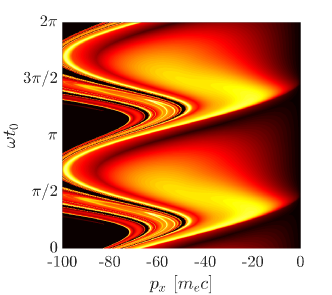
(a) (b)

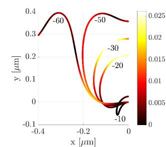
Figure 5: Numerical prediction of maximum $\chi_{\textup{e}}$ attained by electrons of different initial momenta injected into the standing wave formed by a $I=${10}^{22}\text{\,}\mathrm{W}\mathrm{/}\mathrm{c}\mathrm{m}^{2}$$ laser pulse at a different phase. In (a), the maximum emission parameter is indicated by the colour. In (b) trajectories of electrons injected with $p_{\textup{x,0}}=-10,-20,-30,-50$, and $-60\;m_{\textup{e}}c$ into the $\omega t_{0}=3/\pi$ phase are plotted with the colour indicating the instant $\chi_{\textup{e}}$ of the specific electron at that point.

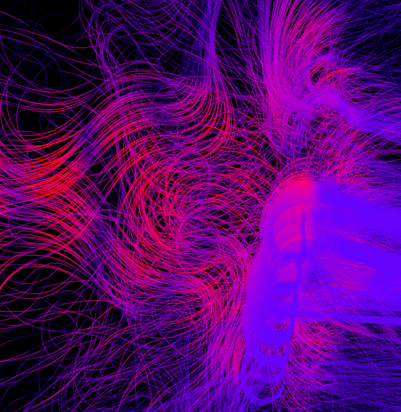
Figure 6: Trajectories of electrons which were accelerated form the front side of a $d=$2\text{\,}\mathrm{\SIUnitSymbolMicro m}$$ target during one of the early half-cycles of a $I=${10}^{22}\text{\,}\mathrm{W}\mathrm{/}\mathrm{c}\mathrm{m}^{2}$$ laser pulse. The simulation area depicted in the illustration spans approximately $x\in(-1,0.5)\,$\mathrm{\SIUnitSymbolMicro m}$$ and $y\in(-1,1)\,$\mathrm{\SIUnitSymbolMicro m}$$. The colour indicates the instant $\chi_{\textup{e}}$ of the specific electron at that point with the scale going from blue (low) to magenta (high). Electrons were selected on the basis of attaining $\chi_{\textup{e}}>0.01$ during one laser pulse half-cycle, then their trajectories were plotted from the beginning of the half-cycle till the end of the simulation. The laser pulse was incoming from the left and injected many electrons into the target on an almost half-circle trajectory, seen in the lower right part of the picture. Upon entering the target, the electrons are not influenced by any strong fields, and continue in a straight line. After they reflect at the back side of the target (far right outside this illustration), some of them, albeit a much lower number, re-enter the interaction area with a high initial velocity, and radiate in the backward direction. This secondary emission happens at a late time of the interaction, and only those electrons that have had been injected in the earliest time arrive soon enough to meet the laser pulse at sufficient intensity to emit any significant amount of radiation – cf. total forward vs. backward emission in figure 13(a).

Equations (2h) and (2i) can be solved numerically, coupled with the relativistic equation of motion of the electron. Figure 5 shows the predicted maximum $\chi_{\textup{e}}$ attained by electrons of different initial momenta injected into the standing wave at different phase which radiate in the space in front of the target in the positive $x$ direction. Around $p_{\textup{x,0}}=-20m_{\textup{e}}c$ at a phase below $\omega t_{0}=\pi/2$, there is a region of stability with respect to these two parameters. Electrons injected with a much lower initial momentum do not radiate at all, while those with a much higher one will never return into the target, and will radiate in the backward direction. Such a high momentum injection cannot be achieved by the interaction of the laser pulse with the front side electrons, and does not appear in the full PIC simulations. However, similar trajectories, depicted in figure 6, can occur when recirculating electrons return form the back side of the target, and enter the area in front of the target while the pulse has a different phase than it would have had in case of direct injection from the front side. This kind of backward emission can be seen in very thin $d\leq$2\text{\,}\mathrm{\SIUnitSymbolMicro m}$$ foil in the late time of the interaction, being caused by the electrons which were injected early, and had enough time to do a subsequent full revolution in the target. Since the electron bunch spreads out in the transverse direction during the recirculation process [30], the returning electrons can be seen as essentially sampling arbitrary pulse phases in the $(\omega t_{0},p_{\textup{x}})$ phase-space.

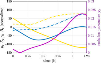
(a) (b)

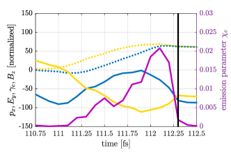
Figure 7: Time evolution of the momentum $p_{\textup{x}}$ of an electron, its relativistic $\gamma$ factor, the $B_{\textup{z}}$ and $E_{\textup{y}}$ fields along its trajectory, and the emission parameter $\chi_{\textup{e}}$ (a) from the simplified theoretical model with the initial momentum corresponding to $\mathcal{E}_{\textup{e}}=$9\text{\,}\mathrm{M}\mathrm{e}\mathrm{V}$$ in a standing wave with a peak intensity $I_{\textup{SW}}=$2\text{\times}{10}^{22}\text{\,}\mathrm{W}\mathrm{/}\mathrm{c}\mathrm{m}^{2}$$ formed by the reflection of a $I=${10}^{22}\text{\,}\mathrm{W}\mathrm{/}\mathrm{c}\mathrm{m}^{2}$$ pulse, and (b) from the Particle-in-Cell simulation of a $I=${10}^{22}\text{\,}\mathrm{W}\mathrm{/}\mathrm{c}\mathrm{m}^{2}$$ laser pulse interacting with a $d=$2\text{\,}\mathrm{\SIUnitSymbolMicro m}$$ CH foil. The momentum $p_{\textup{x}}$ is in the normalized units of $[$\mathrm{m}_{\textup{e}}\mathrm{c}$]$, the electric field $E_{\textup{y}}$ in $[$\mathrm{m}_{\textup{e}}\omega\mathrm{c}\mathrm{/}\mathrm{e}$]$, and the magnetic field $B_{\textup{z}}$ in $[$\mathrm{m}_{\textup{e}}\omega\mathrm{/}\mathrm{e}$]$. Note that the calculation of the theoretical model stops when the electron re-enters the target, while no such limit exists in the PIC simulation, therefore we track the electron after being re-injected to show that $\chi_{\textup{e}}$ indeed drops to zero.

For a sample numerical solution, we calculated the time evolution of the model for the initial momentum of $p_{\textup{x,0}}=-18m_{\textup{e}}c$, which corresponds to the energy $\mathcal{E}_{\textup{e}}=$9\text{\,}\mathrm{M}\mathrm{e}\mathrm{V}$$, injected into the $\pi/3$ phase of a standing wave with peak intensity $I_{\textup{SW}}=$2\text{\times}{10}^{22}\text{\,}\mathrm{W}\mathrm{/}\mathrm{c}\mathrm{m}^{2}$$, which corresponds to the constructive interference of the incoming and reflected parts of an $a_{0}=86,I=${10}^{22}\text{\,}\mathrm{W}\mathrm{/}\mathrm{c}\mathrm{m}^{2}$$ laser pulse. The electron’s trajectory starts and ends at the surface of a target positioned at $x=0$. The model tracks the evolution of the electric $E_{\textup{y}}$ and magnetic $B_{\textup{z}}$ fields along the trajectory of the simulated electron. Together with the electron’s $p_{\textup{x}}$ and its $\gamma$ factor, these constitute the two parts of the simplified equation (2i). The result, shown in figure 7(a), compares favourably to the actual trajectory of an electron, in figure 7(b), selected form the PIC simulation on the basis of similar injection phase, and the initial and final relativistic $\gamma$ factor.

4.3 Electron dynamics

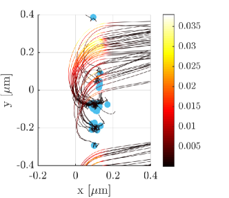
Figure 8: The blue dots represent positions of the particles from the PIC simulation of a $d=$2\text{\,}\mathrm{\SIUnitSymbolMicro m}$$ CH foil, right before they are pulled out of the target, overlaid on the trajectory followed by the respective particle during one half-cycle of a $I=${10}^{22}\text{\,}\mathrm{W}\mathrm{/}\mathrm{c}\mathrm{m}^{2}$$ laser pulse. The trajectory colour shows the value of the emission parameter $\chi_{\textup{e}}$ achieved by the electron along the trajectory.

In order to describe the dynamics of the electrons responsible for the gamma ray emission via inverse Compton scattering, we can compare the results of the numerical solution of equations (2h) and (2i), seen in figure 7(a), to a simulation snapshot zoomed-in to the centre of the interaction area in figure 8. It shows the trajectories of a random sample of electrons which achieve a high value of $\chi_{\textup{e}}$ during one half-cycle of the driving laser pulse. In the simulation, a total of about 18 000 electron macro-particle reach $\chi_{\textup{e}}>0.01$ during this particular half-cycle, and over 99% of them follow trajectories of a similar shape as the one produced by the aforementioned sample numerical solution. At this stage of the interaction, hole boring by the laser pulse has pushed the target surface from $x=0$ to $x\approx$150\text{\,}\mathrm{n}\mathrm{m}$$, the phase of the $E_{\textup{y}}$ field is changing, and a new bunch is about to be accelerated.

First, the electron is pulled out of the target surface, and injected into the standing wave in front of the target when the balance between the $\mathbf{J}\times\mathbf{B}$ force and the force due to the $E_{\textup{x}}$ field is violated. This stage is not covered by the theoretical model, where we instead inject the electron with a specified initial momentum (or a range of momenta, as will be described in the following text), and neglect the $E_{\textup{x}}$ field altogether.

After being injected, the electron is accelerated in the $+y$ direction by the $E_{\textup{y}}$ field, causing a rise in its relativistic $\gamma$ factor. Meanwhile, the phase of the $B_{\textup{z}}$ field changes, causing the increase in the originally negative momentum $p_{\textup{x}}$ up to a moment when $p_{\textup{x}}=0$, and the electron is at the maximum distance $\Delta x\approx$180\text{\,}\mathrm{n}\mathrm{m}$$ away from the actual target surface.

Next, the rising $B_{\textup{z}}$ field transforms the transverse momentum $p_{\textup{y}}$ into the longitudinal $p_{\textup{x}}$ as the electric field $E_{\textup{y}}$ weakens. The relativistic $\gamma$ factor is dominated by the $p_{\textup{x}}$ component – in the normalized units of figure 7, $p_{\textup{x}}\approx\gamma$, and the electron is returning into the target with $p_{\textup{x}}\gg p_{\textup{y}}$.

Maximum $\chi_{\textup{e}}$ parameter is attained right before the re-injection, when $\gamma$ is almost constant as $E_{\textup{y}}$ is decreasing with the impending phase change. The $c\gamma B_{\textup{z}}$ is now the dominant term in equation (2i), but due to the still non-negligible $p_{\textup{y}}$, maximum emission occurs at an angle $\alpha\neq 0$. Right before the re-injection, the $B_{\textup{z}}$ field starts to decrease, and the electrons, which have lost most of their transverse momentum continue to propagate inside the target. The process is about to repeat with the forthcoming laser pulse half-cycle, albeit mirrored with respect to the $x$ axis.

4.4 Emission angle

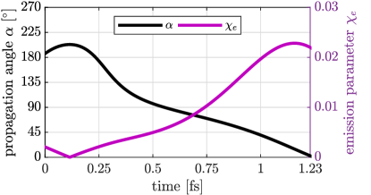
Figure 9: Time evolution of the emission parameter $\chi_{\textup{e}}$, and the propagation angle $\alpha$, measured for the $x$ axis, of the emitting electron in the simplified theoretical model with the initial momentum corresponding to $\mathcal{E}_{\textup{e}}=$9\text{\,}\mathrm{M}\mathrm{e}\mathrm{V}$$ injected into the $\omega t_{0}=\pi/3$ phase of a standing wave with a peak intensity $I_{\textup{SW}}=$2\text{\times}{10}^{22}\text{\,}\mathrm{W}\mathrm{/}\mathrm{c}\mathrm{m}^{2}$$, formed by the reflection of a $I=${10}^{22}\text{\,}\mathrm{W}\mathrm{/}\mathrm{c}\mathrm{m}^{2}$$ pulse.

As we have seen that the maximum emission occurs when the electron is propagating at an angle, we shall now discuss some features of the angular distribution of the emitted photons seen in the theoretical model. Figure 9 shows that the theoretical model predicts an angle $\alpha_{\textup{max}}$, measured from the $x$ axis, where the emission parameter $\chi_{\textup{e}}$ has a maximum for an electron with a given initial momentum. To see how the angle of maximum emission changes in case when a spectrum of electrons would be injected, we first calculate the model values for a range of initial electron momenta. For each energy, we find the time $t_{\textup{max}}$ when the emission parameter has a maximum $\chi_{\textup{e}}^{\textup{max}}=\chi_{\textup{e}}(t_{\textup{max}})$, $\textup{d}\chi_{\textup{e}}/\textup{d}t|_{t_{\textup{max}}}=0$, and the angle $\alpha_{\textup{max}}=\alpha(t_{\textup{max}})$ at which the maximum emission occurs for the given electron energy. Figure 10 shows that there is an optimal initial electron energy $\mathcal{E}_{\textup{e}}^{\textup{opt}}$ which leads to the highest value of the emission parameter at a given laser pulse intensity. Electrons around this optimum are responsible for the majority of the gamma radiation, while those which are too far away, be they slower or faster, would emit considerably less.

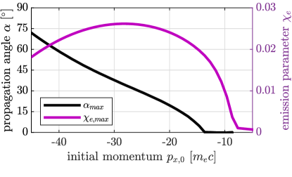
Figure 10: Theoretical model of the maximum emission parameter $\chi_{\textup{e}}^{\textup{max}}$, and the corresponding emission angle $\alpha_{\textup{max}}$ for different initial energies of electrons injected into the $\omega t_{0}=\pi/3$ phase of a standing wave with a peak intensity $I_{\textup{SW}}=$2\text{\times}{10}^{22}\text{\,}\mathrm{W}\mathrm{/}\mathrm{c}\mathrm{m}^{2}$$ formed by the reflection of a $I=${10}^{22}\text{\,}\mathrm{W}\mathrm{/}\mathrm{c}\mathrm{m}^{2}$$ pulse.

Then, we perform a parameter scan over laser pulse intensities, finding the optimal initial electron energy $p_{\textup{x,0}}^{\textup{opt}}(a_{0})$, the emission parameter $\chi_{\textup{e}}^{\textup{max}}$, the emission angle $\alpha_{\textup{max}}$, and the maximum $\gamma$ factor attained by the emitting electron. Figure 11 shows that the maximum $\gamma$ factor is linear in $a_{0}$, thus the maximum emission parameter increases with $\chi_{\textup{e}}\sim a_{0}^{2}$. The angle at the moment when the emission parameter reaches its maximum does not depend on the intensity, and is $\alpha_{\textup{max}}=$$$. If our assumptions hold, one can expect this to be the direction of maximum emission of the ICS gamma rays in the simulations.

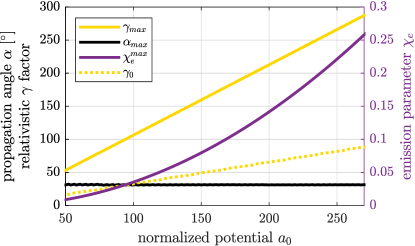
Figure 11: Theoretical model of the maximum emission parameter $\chi_{\textup{e}}^{\textup{max}}$ reached by any electron for a given laser pulse potential $a_{0}=\sqrt{I}$ (where the standing wave maximum intensity is $I_{\textup{SW}}=2I$) with the angle $\alpha_{\textup{max}}$ at which the emission occurs, the relativistic factor $\gamma_{\textup{max}}$ attained by the electron at the point of maximum emission, and the relativistic factor $\gamma_{\textup{0}}$ with which has the electron been injected into the standing wave.

4.5 Angular distribution

In the PIC simulations, the angular distribution of photons emitted via the inverse Compton scattering process in the interaction with a $I=${10}^{22}\text{\,}\mathrm{W}\mathrm{/}\mathrm{c}\mathrm{m}^{2}$$ pulse has a distinct structure with two lobes centred around $\vartheta\simeq$$$ and $\vartheta\simeq$$$. This result is consistent both with previously published simulations [8, 40, 41], and the theoretical model presented in section 4.3.

In the case of very thin foils $d<2c\tau$, recirculating electrons have enough time to make a full revolution and return to the front side of the target while the interaction with the laser pulse is still ongoing. This then leads to an appearance of backward radiation, which is suppressed for thicker foils. The $d=$2\text{\,}\mathrm{\SIUnitSymbolMicro m}$$ target therefore shows a small amount of backward radiation caused by lower energy electrons injected into the target early by the rising part of the pulse, as seen in figure 13(a) Otherwise, since the ICS photons are only emitted from the area in front of an opaque foil target, the angular structure of the resulting radiation does not depend on the target thickness. However, at high intensities, it depends on the target material.

Figure 12 shows that most common direction in which the high energy photons radiate, which is expressed as the mode of the angular distribution of all photons in the 50th energy percentile, corresponds to the theoretical model with $\vartheta\simeq$$$ up to $I=$1\text{\times}{10}^{22}\text{\,}\mathrm{W}\mathrm{/}\mathrm{c}\mathrm{m}^{2}$$. Then, the angle starts to increase, growing faster in the lighter CH foil. This suggests a connection to the hole boring process which is faster at both the high intensities and low-Z targets.

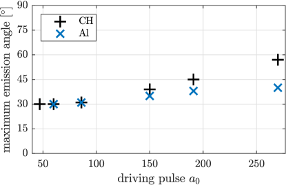
Figure 12: The most prominent direction of propagation of the high energy photons described as the mode of the angular distribution of all photons with energies above the 50th percentile for $d=$2\text{\,}\mathrm{\SIUnitSymbolMicro m}$$ foils from CH and aluminium for driving pulses of different intensities. For $a_{0}=50$, the 50th percentile corresponds to $\mathcal{E}_{\gamma}\sim$1\text{\,}\mathrm{M}\mathrm{e}\mathrm{V}$$, while for $a_{0}=270$, the limit is $\mathcal{E}_{\gamma}\sim$3\text{\,}\mathrm{M}\mathrm{e}\mathrm{V}$$.

The geometry of the front side is defined by the hole boring process [42] since we do not observe any significant decoupling [14] of the ion and electron fronts. As the plasma is being pushed forward, the depth of the ion front increases gradually in the transverse direction towards the centre forming an angled side-wing which stretches from near the focus centre at $y=0$, where the hole reaches the maximum depth, to the region with much lower pulse intensity several micrometers away form the centre, where the original target surface is virtually undisturbed.

As the intensity increases, faster hole boring leads to a larger incidence angle at the sides of the hole, and we cannot assume that the electrons are pulled in front of the target in the direction normal to the polarization of a standing wave. Instead, some enter the interaction area at higher angles. While the radiation is still predominantly forward-going even for the highest intensity $I=${10}^{23}\text{\,}\mathrm{W}\mathrm{/}\mathrm{c}\mathrm{m}^{2}$$ examined in this paper, with increasing intensity, the emission angle increases, backward radiation is enhanced, and the shape of the resulting spectrum, shown in figure 13(b), is approaching that of “transversely oscillating electron synchrotron emission” (TOEE) [41], which itself, in simulations parametrised on plasma density, can be seen as an intermediate stage between the emission from a highly overdense [13] and a near-critical-density [43, 44] target. Detailed exploration of such low density regimes is out of scope of this paper, nevertheless the highest-intensity case presented here bears some similarity to the TOEE process. Furthermore, in this high-intensity short pulse interaction, carrier envelope phase effect leads to a pronounced asymmetry of the emitted radiation.

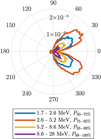
(a) (b)

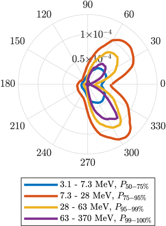
Figure 13: Angular distribution of photons emitted via the inverse Compton scattering process from CH foils with $d=$2\text{\,}\mathrm{\SIUnitSymbolMicro m}$$ at different driving pulse intensities $I=${10}^{22}\text{\,}\mathrm{W}\mathrm{/}\mathrm{c}\mathrm{m}^{2}$$ (a) and $I=${10}^{23}\text{\,}\mathrm{W}\mathrm{/}\mathrm{c}\mathrm{m}^{2}$$ (b). The different curves represent the sum of the energies of all photons in respective energy span in the units of conversion efficiency of the total laser pulse energy into gamma rays in that energy span in given direction per $1\mathrm{°}$ shown on the radial axis. The selection of energy bands in the figures here is not fixed, but differs between simulations to represent exclusive percentile ranges, indicated in the figure legend, to highlight the similarities of the structure of the spectra which, for different intensities, appear at different absolute energy values.

While the hole boring process influences the gamma ray angular distribution in the case of a solid foil with a flat surface, an even more profound effect is revealed in simulations which include pre-plasma, where the interaction moves to a regime of a laser pulse propagating through underdense plasma. This stage is characterized by side injection from a higher density plasma edge formed by electrons pushed away by the ponderomotive force into positively charged channel. Energy stored in the space charge field is then released as periodic pulses of backwards propagating electrons which are in turn slowed by the radiation reaction force [43] and emit high energy photons in the backward direction. This process is called “reinjected electron synchrotron emission”, or RESE [14]. For an exponential pre-plasma profile with the scale length of $l=$1\text{\,}\mathrm{\SIUnitSymbolMicro m}$$, the trajectories of the electrons injected from the lower density regions are chaotic, as seen in figure 14, with no readily identifiable typical features. When the laser pulse reaches the overdense target, hole boring and reflection occur as in the case without pre-plasma, emitting a similar spectrum with the angular distribution featuring the two forward lobes at approximately $\pm$$$. The resulting angular distribution, shown in figure 15 is a combination of both processes. Moreover, since the electrons are accelerated to higher energies in lower density plasma, the emission is enhanced even in the forward direction, where it retains the original structure.

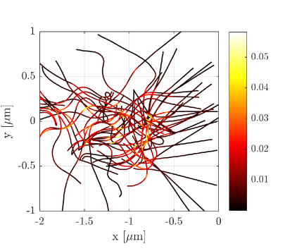
Figure 14: Omnidirectional emission in the presence of pre-plasma is due to the chaotic trajectories of electrons such as those seen in this trajectory snapshot taken during one driving pulse half-cycle (cf. figure 8). The curve colour represents the immediate value of $\chi_{\textup{e}}$ of a given electron at a given point.

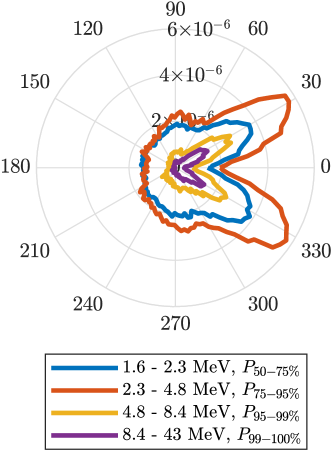
Figure 15: Angular distribution of photons emitted via the inverse Compton scattering process from a $d=$2\text{\,}\mathrm{\SIUnitSymbolMicro m}$$ CH foil with an exponential pre-plasma profile with the scale length of $l=$1\text{\,}\mathrm{\SIUnitSymbolMicro m}$$. The different curves represent the sum of the energies of all photons in respective energy span in the units of conversion efficiency of the total laser pulse energy into gamma rays in that energy span in given direction per $1\mathrm{°}$ shown on the radial axis. The omnidirectional, nearly isotropic, emission is due to the chaotic trajectories of electrons such as those seen in the trajectory snapshot in figure 14 taken during one driving pulse half-cycle.

4.6 Conversion efficiency

Figure 16 shows that in our simulations, the total conversion efficiency obeys the scaling

$$\eta_{{}_{\textup{ICS}}}\sim I^{3/2}$$ (2j)

for both the aluminium and the CH targets. Similar efficiency dependence has been observed in other simulations [40]. As we have established, in equation (2g), the emission parameter scales linearly with the laser pulse intensity, $\chi_{\textup{e}}\sim I$. According to equations (2a) and (2b), the gamma radiation intensity scales as $I_{\textup{rad}}\sim\chi_{\textup{e}}^{\zeta}$ with the power $\zeta=2$ for $\chi_{\textup{e}}\gg 1$, and $\zeta=2/3$ for $\chi_{\textup{e}}\ll 1$. Our simulations reach up to $\chi_{\textup{e}}\approx 1$, a region where neither of the proposed limits are valid. On the one hand, should we lower the intensity to attain $\chi_{\textup{e}}\ll 1$, no ICS emission would be seen at all. On the other, with much higher intensities where $\chi_{\textup{e}}\gg 1$ would be attained, we can no longer speak about an interaction with an opaque over-critical target because of the onset of relativistic transparency. Since we have $\chi_{\textup{e}}\sim I$, equation (2j) suggests that the region in question could be reasonably described by an intermediate empirical value of $\zeta=3/2$.

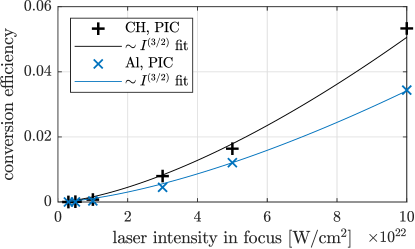
Figure 16: Efficiency of conversion of the total laser pulse energy into all photons emitted via the inverse Compton scattering process from a $d=$2\text{\,}\mathrm{\SIUnitSymbolMicro m}$$ CH and Al foils as a function of the intensity of the driving laser pulse.

4.7 Comparison to Bremsstrahlung

In an experiment, the detectors themselves cannot distinguish between the gamma rays emitted due to bremsstrahlung, which we explored in a previous paper [30], and those emitted due to the inverse Compton scattering process studied here. Both will be seen at the same time, and the distinction has to be based on distilling their unique features from the total spectra.

The first question to be answered is whether the radiation generated by the respective processes would be seen at all. In figure 17(a), we see that for CH foils, ICS dominates already at the lowest intensity $I=$5\text{\times}{10}^{21}\text{\,}\mathrm{W}\mathrm{/}\mathrm{c}\mathrm{m}^{2}$$ where it is detectable. Both its temperature and the number of generated photons rise quickly with the rising intensity, much faster than that of bremsstrahlung. The combination of a thin low-Z target irradiated by such a high intensity pulse clearly favours ICS. As the bremsstrahlung cross section has a strong dependence on the atomic number, rising approximately with $Z^{2}$, using heavier materials should push it to more prominence. Actually, as seen in figure 17(b), the spectrum of bremsstrahlung coming from the Au target dominates over that of the ICS at the laser pulse intensity of $I=${10}^{22}\text{\,}\mathrm{W}\mathrm{/}\mathrm{c}\mathrm{m}^{2}$$. A more precise summary of the measured values, shown in table 2, reveals that the $d=$2\text{\,}\mathrm{\SIUnitSymbolMicro m}$$ Au foil is indeed a cross point where the total conversion efficiencies of the two processes are comparable. Similarly, a comparison can be made between the ICS emission from the $d=$2\text{\,}\mathrm{\SIUnitSymbolMicro m}$$ Al foil, and the bremsstrahlung emission from a $d=$5\text{\,}\mathrm{\SIUnitSymbolMicro m}$$ Al foil. Additionally, the effect of lowered absorption and hence a much lower conversion efficiency into the ICS gamma rays due to lower electron density can be seen in comparison between the different ionizations of the Au foil.

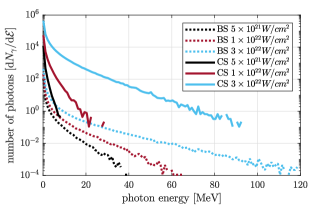
(a) (b)

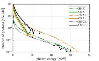
Figure 17: Comparison of bremsstrahlung and inverse Compton scattering spectra in interactions of (a) laser pulses of different intensities with a $d=$2\text{\,}\mathrm{\SIUnitSymbolMicro m}$$ thick CH foil, and (b) a $I=${10}^{22}\text{\,}\mathrm{W}\mathrm{/}\mathrm{c}\mathrm{m}^{2}$$ laser pulse with $d=$2\text{\,}\mathrm{\SIUnitSymbolMicro m}$$ thick foils made of different materials – C⁶⁺H⁺, Al¹³⁺, and Au⁵¹⁺.

		in [$10^{-6}$] at $t=$170\text{\,}\mathrm{f}\mathrm{s}$$
material	thickness	00 $\eta_{{}_{\textup{BS}}}$	$\eta_{{}_{\textup{ICS}}}$
C6+H+	$2\text{\,}\mathrm{\SIUnitSymbolMicro m}$	000 1.6	690
	$5\text{\,}\mathrm{\SIUnitSymbolMicro m}$	000 3.5
Al13+	$2\text{\,}\mathrm{\SIUnitSymbolMicro m}$	000 5.2	240
	$5\text{\,}\mathrm{\SIUnitSymbolMicro m}$	00 12 .0
Au51+	$2\text{\,}\mathrm{\SIUnitSymbolMicro m}$	00 89 .0	00 75
	$5\text{\,}\mathrm{\SIUnitSymbolMicro m}$	190 .0
Au30+	$5\text{\,}\mathrm{\SIUnitSymbolMicro m}$	140 .0	00 31

Table 2: Efficiency of conversion of the laser pulse energy into the energy of all photons generated by the bremsstrahlung process $\eta_{{}_{\textup{BS}}}$, and the inverse Compton scattering process $\eta_{{}_{\textup{ICS}}}$ for targets of different materials irradiated by a $a_{0}=86,I=${10}^{22}\text{\,}\mathrm{W}\mathrm{/}\mathrm{c}\mathrm{m}^{2}$$ laser pulse. For foils with $d>$2\text{\,}\mathrm{\SIUnitSymbolMicro m}$$, the conversion by inverse Compton scattering does not depend on the target thickness, therefore the same values can be used for comparison of the $d=$2\text{\,}\mathrm{\SIUnitSymbolMicro m}$$ and the $d=$5\text{\,}\mathrm{\SIUnitSymbolMicro m}$$ foil.

5 Conclusions

We have studied the emission of gamma rays by inverse Compton scattering in interactions of a short intense laser pulse with a thin foil target via 2D PIC simulations. The ICS process dominates over bremsstrahlung in low-Z targets already at a threshold intensity $I\approx$3\text{\times}{10}^{21}\text{\,}\mathrm{W}\mathrm{/}\mathrm{c}\mathrm{m}^{2}$$ under which no ICS generated gamma rays are seen at all. Spectra of the gamma rays produced in interactions with different driving pulse intensities show a linear dependence of the ICS produced gamma ray temperature on the intensity $T_{\gamma}\sim a_{0}^{2}\sim I$, at least in the studied intensity range $I=$3\text{\times}{10}^{21}$-${10}^{23}\text{\,}\mathrm{W}\mathrm{/}\mathrm{c}\mathrm{m}^{2}$$. As the ICS process takes place in front of the target in the evolving field of the laser pulse, the relation between the temperature of the electrons and that of the resulting gamma rays is provided as an empirical observation only.

The radiation is forward going with two lobes centred at approximately $\vartheta\approx$$$. The angular distribution of the emission is dictated by the dynamics of the electrons in the field of the laser pulse in front of the target, thus for sufficiently thick $d\gtrsim$2\text{\,}\mathrm{\SIUnitSymbolMicro m}$$ targets, there is no change in its structure with increasing thickness. A simple theoretical model which assumes the movement of an electron in a planar standing wave formed in the front side by the interaction of the incoming and reflected parts of the laser pulse predicts the photon propagation angle $\vartheta=$$$ regardless of the laser pulse intensity. This is confirmed by the simulations up to $I\approx${10}^{22}\text{\,}\mathrm{W}\mathrm{/}\mathrm{c}\mathrm{m}^{2}$$. As the intensity grows further, the propagation angle increases since the assumptions of the theoretical model break down due to hole boring. When the hole in the surface is sufficiently deep, the electrons injected from its sides meet the laser pulse in a different phase, and travel along a different trajectory before being reinjected near the centre of the hole. Moreover, when the hole’s depth is comparable to the laser pulse wavelength $\lambda=$1\text{\,}\mathrm{\SIUnitSymbolMicro m}$$, the combined field of the incoming and the reflected parts of the laser pulse cannot be adequately described by that of a planar standing wave which would form in front of a flat surface. Efficiency of conversion of the driving laser pulse energy into that of the gamma rays generated by ICS shows super-linear scaling with intensity $\eta_{{}_{\textup{ICS}}}\sim I^{3/2}$ in the studied intensity range.

Comparing the results to our previous work, where we show that targets made of materials with a higher atomic number, while exhibiting a lower absorption, still show a significant increase of gamma ray production by bremsstrahlung [30], we see that the lower absorption also affects the ICS process which does not directly depend on the atomic number. Lower-Z targets give out much more ICS gamma rays with a crossing point being a $d=$2\text{\,}\mathrm{\SIUnitSymbolMicro m}$$ thick Au⁵¹⁺ target irradiated by a $I=${10}^{22}\text{\,}\mathrm{W}\mathrm{/}\mathrm{c}\mathrm{m}^{2}$$ laser pulse, for which the two processes exhibit roughly the same conversion efficiency.

References

References

- [1] Weber S, Bechet S, Borneis S, Brabec L, Bučka M, Chacon-Golcher E, Ciappina M, DeMarco M, Fajstavr A, Falk K, Garcia E R, Grosz J, Gu Y J, Hernandez J C, Holec M, Janečka P, Jantač M, Jirka M, Kadlecova H, Khikhlukha D, Klimo O, Korn G, Kramer D, Kumar D, Lastovička T, Lutoslawski P, Morejon L, Olšovcová V, Rajdl M, Renner O, Rus B, Singh S, Šmid M, Sokol M, Versaci R, Vrána R, Vranic M, Vyskočil J, Wolf A and Yu Q 2017 Matter and Radiation at Extremes 2 149–176 ISSN 2468-080X
- [2] Hernandez-Gomez C, Blake S P, Chekhlov O, Clarke R J, Dunne A M, Galimberti M, Hancock S, Heathcote R, P Holligan, Lyachev A, Matousek P, Musgrave I O, Neely D, Norreys P A, Ross I, Tang Y, Winstone T B, Wyborn B E and Collier J 2010 Journal of Physics: Conference Series 244 032006 ISSN 1742-6596
- [3] Zou J P, Blanc C L, Papadopoulos D N, Chériaux G, Georges P, Mennerat G, Druon F, Lecherbourg L, Pellegrina A, Ramirez P, Giambruno F, Fréneaux A, Leconte F, Badarau D, Boudenne J M, Fournet D, Valloton T, Paillard J L, Veray J L, Pina M, Monot P, Chambaret J P, Martin P, Mathieu F, Audebert P and Amiranoff F 2015 High Power Laser Science and Engineering 3 ISSN 2095-4719, 2052-3289
- [4] Danson C, Hillier D, Hopps N and Neely D 2015 High Power Laser Science and Engineering 3 ISSN 2095-4719, 2052-3289
- [5] Bernstein M J and Comisar G G 1970 Journal of Applied Physics 41 729–733 ISSN 0021-8979
- [6] Ritus V I 1985 Journal of Soviet Laser Research 6 497–617 ISSN 0270-2010, 1573-8760
- [7] Lau Y Y, He F, Umstadter D P and Kowalczyk R 2003 Physics of Plasmas 10 2155 ISSN 1070664X
- [8] Nakamura T, Koga J K, Esirkepov T Z, Kando M, Korn G and Bulanov S V 2012 Physical Review Letters 108 ISSN 0031-9007, 1079-7114
- [9] Gu Y J, Jirka M, Klimo O and Weber S 2019 Matter and Radiation at Extremes 4 064403 ISSN 2468-2047
- [10] Bell A R and Kirk J G 2008 Physical Review Letters 101 ISSN 0031-9007, 1079-7114
- [11] Bulanov S S, Schroeder C B, Esarey E and Leemans W P 2013 Physical Review A 87 ISSN 1050-2947, 1094-1622
- [12] Di Piazza A, Müller C, Hatsagortsyan K Z and Keitel C H 2012 Reviews of Modern Physics 84 1177–1228
- [13] Ridgers C P, Brady C S, Duclous R, Kirk J G, Bennett K, Arber T D, Robinson A P L and Bell A R 2012 Physical Review Letters 108 ISSN 0031-9007, 1079-7114
- [14] Brady C S, Ridgers C P, Arber T D, Bell A R and Kirk J G 2012 Physical Review Letters 109 245006
- [15] Zhidkov A, Koga J, Sasaki A and Uesaka M 2002 Physical Review Letters 88 185002
- [16] Ta Phuoc K, Corde S, Thaury C, Malka V, Tafzi A, Goddet J P, Shah R C, Sebban S and Rousse A 2012 Nature Photonics 6 308–311 ISSN 1749-4885, 1749-4893
- [17] Englert T J and Rinehart E A 1983 Physical Review A 28 1539–1545
- [18] Bula C, McDonald K T, Prebys E J, Bamber C, Boege S, Kotseroglou T, Melissinos A C, Meyerhofer D D, Ragg W, Burke D L, Field R C, Horton-Smith G, Odian A C, Spencer J E, Walz D, Berridge S C, Bugg W M, Shmakov K and Weidemann A W 1996 Physical Review Letters 76 3116–3119
- [19] Chen S Y, Maksimchuk A and Umstadter D 1998 Nature 396 653–655 ISSN 1476-4687
- [20] Schwoerer H, Liesfeld B, Schlenvoigt H P, Amthor K U and Sauerbrey R 2006 Physical Review Letters 96 ISSN 0031-9007, 1079-7114
- [21] Malka G, Aleonard M M, Chemin J F, Claverie G, Harston M R, Scheurer J N, Tikhonchuk V, Fritzler S, Malka V, Balcou P, Grillon G, Moustaizis S, Notebaert L, Lefebvre E and Cochet N 2002 Physical Review E 66 066402
- [22] Chen S, Powers N D, Ghebregziabher I, Maharjan C M, Liu C, Golovin G, Banerjee S, Zhang J, Cunningham N, Moorti A, Clarke S, Pozzi S and Umstadter D P 2013 Physical Review Letters 110 ISSN 0031-9007, 1079-7114
- [23] Sarri G, Corvan D J, Schumaker W, Cole J M, Di Piazza A, Ahmed H, Harvey C, Keitel C H, Krushelnick K, Mangles S P D, Najmudin Z, Symes D, Thomas A G R, Yeung M, Zhao Z and Zepf M 2014 Physical Review Letters 113 224801
- [24] Yan W, Fruhling C, Golovin G, Haden D, Luo J, Zhang P, Zhao B, Zhang J, Liu C, Chen M, Chen S, Banerjee S and Umstadter D 2017 Nature Photonics 11 514–520 ISSN 1749-4893
- [25] Cole J M, Behm K T, Gerstmayr E, Blackburn T G, Wood J C, Baird C D, Duff M J, Harvey C, Ilderton A, Joglekar A S, Krushelnick K, Kuschel S, Marklund M, McKenna P, Murphy C D, Poder K, Ridgers C P, Samarin G M, Sarri G, Symes D R, Thomas A G R, Warwick J, Zepf M, Najmudin Z and Mangles S P D 2018 Physical Review X 8 ISSN 2160-3308
- [26] Poder K, Tamburini M, Sarri G, Di Piazza A, Kuschel S, Baird C D, Behm K, Bohlen S, Cole J M, Corvan D J, Duff M, Gerstmayr E, Keitel C H, Krushelnick K, Mangles S P D, McKenna P, Murphy C D, Najmudin Z, Ridgers C P, Samarin G M, Symes D R, Thomas A G R, Warwick J and Zepf M 2018 Physical Review X 8 031004
- [27] Malka G and Miquel J L 1996 Physical Review Letters 77 75–78
- [28] Pukhov A 2001 Physical Review Letters 86 3562–3565
- [29] Arber T D, Bennett K, Brady C S, Lawrence-Douglas A, Ramsay M G, Sircombe N J, Gillies P, Evans R G, H Schmitz, Bell A R and Ridgers C P 2015 Plasma Physics and Controlled Fusion 57 113001 ISSN 0741-3335
- [30] Vyskočil J, Klimo O and Weber S 2018 Plasma Physics and Controlled Fusion 60 054013 ISSN 0741-3335, 1361-6587
- [31] Kirk J G, Bell A R and Arka I 2009 Plasma Physics and Controlled Fusion 51 085008
- [32] Sauter F 1931 Zeitschrift für Physik 69 742–764 ISSN 0044-3328
- [33] Schwinger J 1951 Physical Review 82 664–679 ISSN 0031-899X
- [34] Shen C S and White D 1972 Physical Review Letters 28 455–459
- [35] Nikishov A and Ritus V 1964 Sov. Phys. JETP 19 529–541
- [36] Wilks S C, Kruer W L, Tabak M and Langdon A B 1992 Physical Review Letters 69 1383–1386
- [37] Yee K 1966 IEEE Transactions on Antennas and Propagation 14 302–307 ISSN 0018-926X
- [38] Boris J P 1970 Proceeding of Fourth Conference on Numerical Simulations of Plasmas
- [39] Duclous R, Kirk J G and Bell A R 2010 Plasma Physics and Controlled Fusion 53 015009
- [40] Ji L L, Pukhov A, Nerush E N, Kostyukov I Y, Shen B F and Akli K U 2014 Physics of Plasmas 21 023109 ISSN 1070-664X
- [41] Chang H X, Qiao B, Zhang Y X, Xu Z, Yao W P, Zhou C T and He X T 2017 Physics of Plasmas 24 043111 ISSN 1070-664X
- [42] Robinson A P L, Gibbon P, Zepf M, Kar S, Evans R G and Bellei C 2009 Plasma Physics and Controlled Fusion 51 024004 ISSN 0741-3335, 1361-6587
- [43] Brady C S, Ridgers C P, Arber T D and Bell A R 2013 Plasma Physics and Controlled Fusion 55 124016 ISSN 0741-3335
- [44] Brady C S, Ridgers C P, Arber T D and Bell A R 2014 Physics of Plasmas 21 033108 ISSN 1070-664X