Spatial segregation of massive clusters in dwarf galaxies

Abstract

The relative average minimum projected separations of star clusters in the Legacy ExtraGalactic UV Survey (LEGUS) and in tidal dwarfs around the interacting galaxy NGC 5291 are determined as a function of cluster mass to look for cluster-cluster mass segregation. Class 2 and 3 LEGUS clusters, which have a more irregular internal structure than the compact and symmetric class 1 clusters, are found to be mass segregated in low mass galaxies, which means that the more massive clusters are systematically bunched together compared to the lower mass clusters. This mass segregation is not present in high-mass galaxies nor for class 1 clusters. We consider possible causes for this segregation including differences in cluster formation and scattering in the shallow gravitational potentials of low mass galaxies.

1 Introduction

Compact star clusters usually form inside more extended associations of young stars (Feitzinger & Galinski, 1987; Elmegreen & Efremov, 1997; Hunter, 1999; Maíz-Apellániz, 2001; Lada & Lada, 2003; Elmegreen et al., 2006; Elmegreen, 2008; Portegies Zwart et al., 2010; Krumholz et al., 2019), as part of a hierarchical structure for star formation that resembles the distribution of dense interstellar clouds (Scalo, 1985; Fleck, 1996; Elmegreen & Falgarone, 1996; Cartwright & Whitworth, 2004). The relative positions and ages of these clusters follow power-law correlations (Efremov & Elmegreen, 1998; de la Fuente Marcos & de la Fuente Marcos, 2009; Grasha et al., 2017a) suggesting this hierarchy is the result of turbulent motions with self-gravity dominating the densest phase.

While this basic structure is well observed, there has been little effort to quantify the spatial correlation as a function of cluster mass. We do not know, for example, if the most massive clusters group together with lower mass clusters surrounding them. Such mass segregation can be an important constraint on cluster formation models and an indicator of the history of the region, including competitive (e.g., Zinnecker, 1982; Bonnell et al., 1997) or cooperative (Elmegreen et al., 2014) accretion of gas into the clusters, or density-dependent cloud masses (Alfaro & Román-Zúñiga, 2018). Mutual cluster attraction leading to coalescence in dense regions (Lahén et al., 2019) might also be indicated.

Here we describe a new metric for mass-dependent clustering that has the potential to reveal whether clusters segregate according to mass. We apply this metric to clusters in the Legacy ExtraGalactic UV Survey (LEGUS) database (Calzetti et al., 2015) and, by comparison, to clusters in tidal dwarfs around the interacting galaxy NGC 5291 (Fensch et al., 2019). These tidal dwarfs have HST images and the highest number of clusters observed so far for this type of galaxy.

2 Method

2.1 The Relative Average Minimum Projected Separation

To gain insight on mass segregation among high and low mass clusters, we consider the average minimum projected separation between clusters as a function of cluster mass. We denote this quantity, corrected for galaxy inclination, by ${\bar{D}}_{\rm min}(M)$, where the bar denotes the average for all clusters of a particular mass $M$, and the subscript “min” denotes the minimum distance $D$ to these other cluster. For a random distribution of cluster positions, this separation is about equal to the inverse square root of the average projected cluster density. In addition, we denote the number of clusters in a logarithmic mass interval by $N(M)d\log M$. For a uniform random distribution of clusters of all masses, ${\bar{D}}_{\rm min}(M)$ multiplied by $N(M)^{1/2}$ is independent of $M$. The mass distribution function for clusters and incompleteness at low mass both enter ${\bar{D}}_{\rm min}(M)$ and $N(M)$ in the same way, cancelling out.

If high mass clusters of mass $M_{\rm H}$ are more bunched together than low mass clusters of mass $M_{\rm L}$, then

$$N(M_{\rm H})^{1/2}{\bar{D}}_{\rm min}(M_{\rm H})<N(M_{\rm L})^{1/2}{\bar{D}}_{\rm min}(M_{\rm L}).$$ (1)

Thus, a plot of $N(M)^{1/2}{\bar{D}}_{\rm min}(M)$ versus $M$ indicates the relative segregation of different masses.

For comparisons among different regions in a galaxy or different galaxies, the above quantity should be normalized to the region size, which we take to be the average projected separation (corrected for galaxy inclination) between the clusters in the lowest mass interval, ${\bar{D}}(M_{\rm low})$. This interval is chosen because generally it has the most clusters and gives the most accurate region size. Thus, the quantity to consider as a function of mass is the relative average minimum projected separation (RAMPS) corrected for galaxy inclination,

$$RAMPS(M)=N(M)^{1/2}{\bar{D}}_{\rm min}(M)/{\bar{D}}(M_{\rm low}).$$ (2)

Another measure of relative cluster separation is the two-point correlation function (e.g., Bastian et al., 2009; Grasha et al., 2017b), which determines the relative proportions of all separations. The RAMPS differs because it uses only the nearest distances.

2.2 Testing the RAMPS

A fractal hierarchical model shows the trends in RAMPS. This model is made on a $512\times 512$ square grid of total size 1 with 8 levels of hierarchy starting with a $4\times 4$ grid of cells at the top in level $i=2$ (see Elmegreen, 2018). At each level $i$ there is a probability $p$ of choosing a cell that will be further subdivided into $2\times 2$ cells in the next lower level. This probability depends on the fractal dimension $D_{\rm f}$ and is given by $p=2^{D_{\rm f}-2}$. To choose a cell, a random number between 0 and 1 is generated and compared to $p$; if the random number is smaller than $p$, we choose the cell. Note that a fractal dimension $D_{\rm f}=2$ causes all cells to be chosen ($p=1$), filling the square grid completely in two-dimensions. For the model we use $D_{\rm f}=1.3$ because that matches the observations of interstellar clouds (Elmegreen & Falgarone, 1996). Each level sub-divides only the cells chosen at the next higher level. For level $i$ from 2 to 9, the size of the cell is $1/2^{i}$ and the total number of cells is $2^{i}\times 2^{i}$, although only the fraction $p$ are chosen at each level.

We assign a mass to each of the cells at all levels, considering that the cell center represents the position of a star cluster in the hierarchy of young stellar structures. To give mass segregation, uniformity, or inverse segregation, we let the cluster mass $M$ scale with the level $i$ such that $M=M_{0}\mu^{i}$ where $\mu=10^{0.5}$, 1, or $10^{-0.5}$ for $i=2,...,6$ in these three cases respectively. To keep the masses in the range of $10^{3}\;M_{\odot}$ to $10^{5}\;M_{\odot}$, we set $M_{0}=10^{2}\;M_{\odot}$ and $10^{6}\;M_{\odot}$ for the segregation and inverse segregation cases. For the uniform case, we let $\log M_{0}$ be a random number uniformly distributed between 3 and 5. Because cells at levels with larger $i$ are on average closer together within their hierarchies than cells at lower $i$ within the same hierarchy, the segregation of high mass clusters to denser average regions corresponds to a greater proportion of massive clusters at large $i$. This is why $\mu>1$ corresponds to mass segregation and $\mu<1$ corresponds to inverse mass segregation, where massive clusters systematically avoid each other compared to low mass clusters.

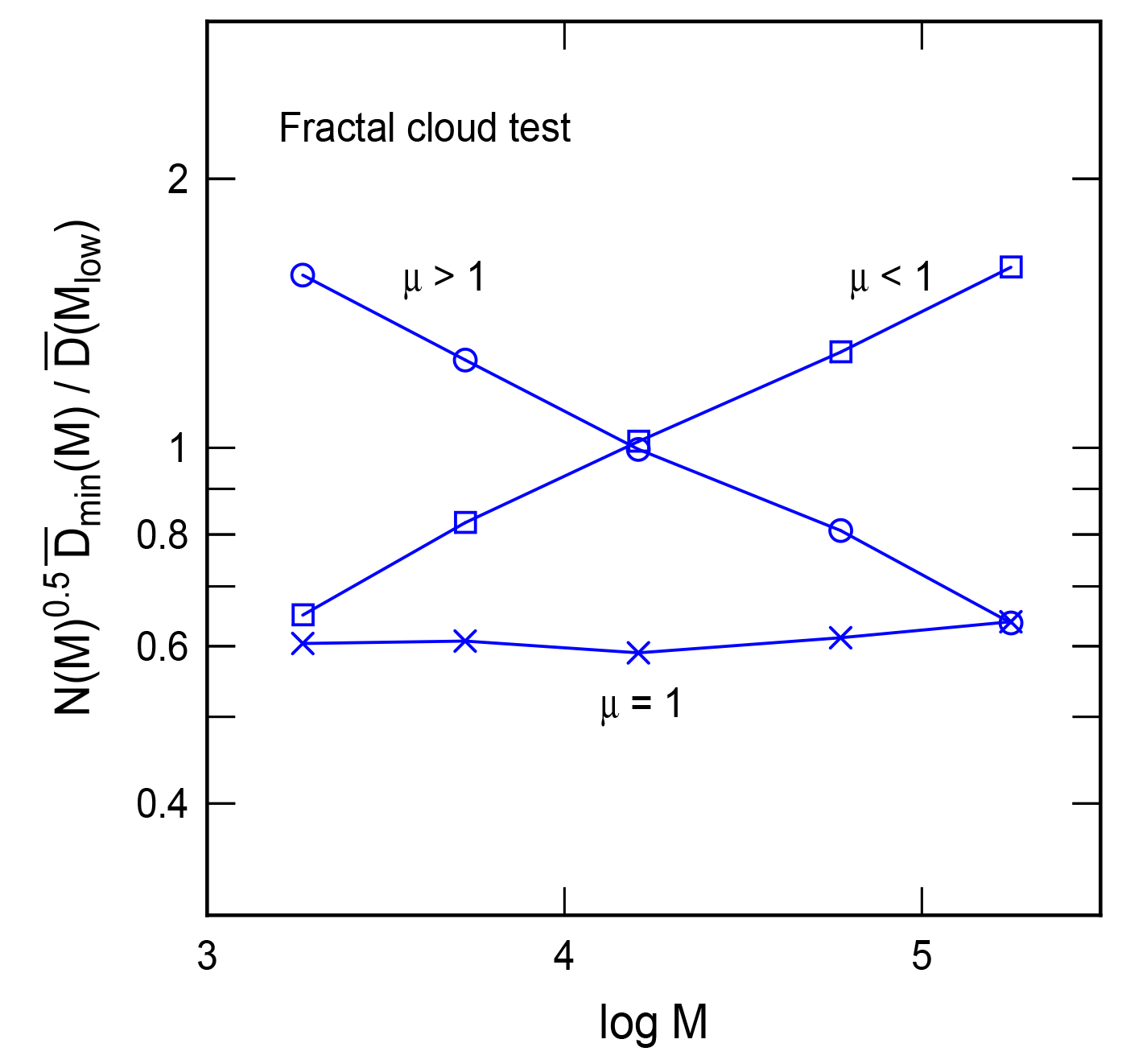
Figure 1: (top) The relative average minimum projected separations (RAMPS) between clusters are plotted versus the cluster mass for randomly positioned clusters in a hierarchical fractal distribution. The mass units are arbitrary. Increasing slopes indicate that low-mass clusters are preferentially clumped together, while decreasing slopes indicate that high-mass clusters are clumped together. Randomly positioned clusters give a flat slope.

Figure 1 shows the RAMPS function for the three values of $\mu$. Mass segregation with $\mu>1$ has a negative slope and inverse mass segregation has a positive slope. Random mass in the hierarchy corresponds to a horizontal line in the figure. The way to interpret the negative slope is that the nearest neighbor high mass cluster to another high mass cluster is closer than the average cluster spacing would be at that mass if they were randomly distributed over the whole region.

3 Data

Catalogs in the Hubble Space Telescope LEGUS survey were used to obtain the positions, ages and masses of measured clusters (Calzetti et al., 2015; Adamo et al., 2017), considering Padova stellar evolution models with starburst extinction curves. To keep the sample as free as possible from fading effects with age, we consider only clusters more massive than a distance-dependent limit, $M_{\rm limit}$, and younger than 125 Myr. For almost all galaxies in LEGUS, the lower limit to the detectable mass at 125 Myr age is $94D_{\rm Mpc}^{2}\;M_{\odot}$ for distance $D_{\rm Mpc}$ in Mpc. This mass corresponds to an absolute V-band magnitude of $M_{\rm v}=-6.0$. For a typical distance of 6 Mpc, the typical mass limit is $3400\;M_{\odot}$. Then, for the entire sample, there are 14 galaxies that have 35 or more such clusters in classes 2 or 3 and which span a factor of $10^{1.5}$ or more in mass. These galaxies and their cluster counts are listed in Table 1 along with the RAMPS slopes. Galaxy distances, star formation rates and stellar masses are from Calzetti et al. (2015), as are inclinations (not listed). Galaxy position angles are from various sources such as the Third Reference Catalog of Bright Galaxies (de Vaucouleurs et al., 1991) and the LITTLE THINGS survey (Hunter et al., 2012) when available, and measured from LEGUS images at the LEGUS web site when not available, all verified by measurements on the Digitized Sky Survey.

Table 1 also lists the 11 galaxies that have 35 or more class 1 clusters spanning a factor of $10^{1.5}$ or more in mass within the same age and mass limits. Similarly, the table lists the cluster counts and RAMPS slopes considering only class 2 types alone and only class 3 types alone. Class 1 clusters are compact, class 2 are somewhat elongated, and class 3 are multi-core (Adamo et al., 2017). The galaxies span a factor of $\sim 100$ in star formation rate and stellar mass, so they represent a fair sample of spiral and dwarf galaxy types.

The clusters were first divided into logarithmic mass intervals of 0.5 dex; the number of bins in Table 1 represents the number of these intervals spanned by the cluster masses. As for the random trial discussed above, the projected separations between each cluster and all the other clusters in the same mass interval (corrected for galaxy inclination) were determined and the minimum of these separations was noted. This minimum represents the distance between each particular cluster and its nearest cluster of the same mass. The average of these minimum distances was then determined for each mass interval. After multiplication by the square root of the number of clusters in the mass interval and division by the average separation in the lowest mass interval, we obtain the RAMPS.

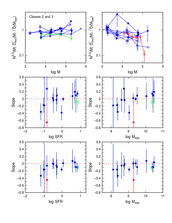
Figure 2: (top) The RAMPS are plotted versus the cluster mass $M$ (in $M_{\odot}$) for LEGUS clusters in classes 2 and 3 (blue lines) and for NGC 5291 (red line) clusters. The RAMPS are dimensionless. Error bars are from the student-t distribution at 90% probability; they are symmetric around the linear value of the RAMPS but asymmetric here when plotted logarithmically (points with no error bars have only 2 clusters in that mass interval). Cluster masses are randomly offset from the center of the mass bin for clarity; different galaxies have different symbols. Increasing RAMPS are on the left and decreasing RAMPS are on the right. (middle, bottom) The slopes of the RAMPS are shown versus the total galaxy star formation rates (in $M_{\odot}$ yr^-1) and galaxy stellar masses (in $M_{\odot}$). The middle panels are for RAMPS calculated using equal $\log(M)$ intervals, as in the top panels, while the bottom panels are for RAMPS calculated using equal numbers of clusters in each mass interval. Low-mass galaxies tend to have decreasing RAMPS, indicating a greater tendency for high mass clusters to collect together compared to low mass clusters. The green line and crosses on the top left and green crosses in the middle and bottom panels are for NGC 5194 clusters determined by Machine Learning; the blue crosses on the top left are for NGC 5194 visual identifications.

Figure 2 shows the RAMPS for the LEGUS clusters in classes 2 and 3, divided into those with increasing or nearly constant average slopes on the left and those with decreasing average slopes on the right. These slopes are determined from the whole mass range, which, e.g., for 4 bins, corresponds to a factor of $\sim 100$.

The middle panels in Figure 2 show the RAMPS slope versus the star formation rate (SFR) (left) and the galaxy stellar mass $M_{\rm star}$ (right). There is an increasing trend in both panels. The slopes of these trends were determined by least squares linear fits with uncertainties given by the student-t distribution at 90% probability. Corresponding $\chi^{2}$ values are from the sum of the squared differences between the RAMPS slopes and the linear fits, normalized to the uncertainties in the slopes. The result is a slope of $0.14\pm 0.13$ with $\chi_{\rm r}^{2}=6.5$ for 12 degrees of freedom (DOF) in the plot of RAMPS slope versus $\log(SFR)$, and $0.14\pm 0.10$ with $\chi^{2}=4.9$ for 12 DOF in the plot of RAMPS slope versus $\log M_{\rm star}$. These $\chi^{2}$ values are smaller than the number of DOF, which is number of RAMPS values minus 2, indicating reasonably good fits. A summary is in Table 1.

The bottom panels in Figure 2 show the RAMPS slopes calculated with an equal number of clusters in each of 6 cluster mass intervals (rather than equal $\log(M)$ intervals). The upward trends are present for this binning too, although slightly smaller. Still, their slopes (Table 1) are within the error bars of the slopes in the middle panels.

The correlations between the slope of the RAMPS and the galaxy SFR or stellar mass imply that low mass galaxies have their most massive class 2-3 clusters closer together than average, whereas high mass galaxies have all cluster masses randomly distributed.

Inclination errors could affect the results, but a recalculation of the class 2+3 case with zero inclinations gave about the same slopes: $0.16\pm 0.14$ versus $\log{SFR}$ and $0.16\pm 0.11$ versus $\log(M_{\rm star})$. The $\chi^{2}$ values were much higher without inclination corrections, however, 31 and 18, respectively.

The clusters were identified by eye for all galaxies, but for NGC 5194, clusters were also identified with Machine Learning (ML) techniques, using the visual identifications as a training set (Messa et al., 2018; Grasha et al., 2019). There are more ML clusters than visual clusters for this galaxy, but the slope of the RAMPS is about the same in both cases. The green points in the bottom of Figure 2 and the green crosses and line in the top left are for clusters identified by ML in NGC 5194, compared to the blue points at the same SFR and stellar mass on the bottom and the blue crosses on the top left.

We also considered clusters in the tidal dwarf galaxies connected with the interacting galaxy NGC 5291. These were obtained from the study by Fensch et al. (2019) with distances between the clusters determined by assuming zero inclination and position angle as these are highly irregular galaxies. Among their sample of 272 clusters with masses less than $3\times 10^{5}\;M_{\odot}$ and not category 0 (which are excluded because they have more than two HST passbands with only upper limits on the flux), we include all 106 clusters with masses larger than $10^{4}\;M_{\odot}$ and ages less than 100 Myr. These limits avoid the loss of clusters from fading. There are several dwarfs in the collision debris but we can treat all of them as one large distribution to derive the slope of the RAMPS because the nearest cluster to any given cluster of the same mass is likely to be inside the same tidal dwarf. The other factors in RAMPS, $N(M)$ and $D_{\rm low}$, are constant and do not affect the slope. The red segmented line and red points in Figure 2 show the results for NGC 5291. The RAMPS for NGC 5291 has a negative slope like the other dwarf galaxies.

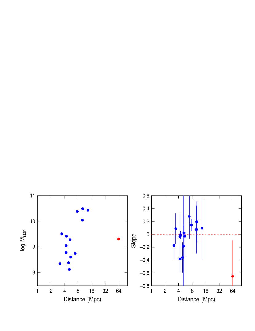
Figure 3: (left) Galaxy stellar mass in $M_{\odot}$ is shown as a function of galaxy distance in Mpc. (right) The slope of the RAMPS for class 2 and 3 clusters is shown as a function of distance. The blue points are LEGUS galaxies and the red point is for tidal dwarfs around NGC 5291. For the LEGUS galaxies, there is a correlation between galaxy mass and distance, and so a resulting correlation appears between RAMPS slope and distance, but the RAMPS does not appear to be biased for distance by itself.

Figure 3 shows $M_{\rm star}$ versus distance, with the expected trend for lower mass galaxies, which are more common, to be closer. Because of this, the closer galaxies also have more negative slopes in the RAMPS, as shown in the right-hand panel. These distance trends are not the cause of the varying slopes for RAMPS, however. The cluster separations are well resolved for all of the galaxy distances, and the cluster mass ranges are about the same scaled for distance. Moreover, the distance to NGC 5291 (red points in Figure 3) is larger than even the massive galaxies in LEGUS and yet the slope of its RAMPS is negative, like the closer dwarfs.

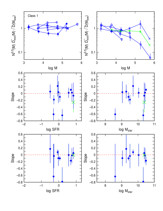
Figure 4: (top) The RAMPS are plotted versus the cluster mass ($M_{\odot}$) for LEGUS clusters in class 1. (middle, bottom) The slopes of the RAMPS are shown versus the total galaxy star formation rates (in $M_{\odot}$ yr^-1) and galaxy stellar masses (in $M_{\odot}$). Unlike the class 2 and 3 clusters in Figure 2, the class 1 clusters appear to be randomly distributed for all galaxy masses. The green line and crosses on the top right and the green crosses in the middle and bottom panels are for NGC 5194 clusters discovered by Machine Learning. As in Figure 2, the middle panels are for RAMPS calculated with equal $\log(M)$ intervals of cluster mass, and the bottom panels are for RAMPS calculated with equal numbers of clusters in each mass interval.

The RAMPS for class 1 clusters in LEGUS is shown in Figure 4. Again the positive and negative slopes are separated in the two top panels, but now the slopes are all around 0, as also shown in the middle and bottom panels. Evidently the class 1 clusters have different grouping properties than the class 2 and 3 clusters. Separate plots for class 2 clusters and for class 3 clusters alone (not shown) repeat the correlation in Figure 2, which was for the combined classes. The number of clusters and RAMPS slopes for these separate classes are given in Table 1 for completeness.

We also determined the RAMPS for only the young class 1 clusters with ages less than 30 Myr (not shown); these had no obvious trends with galaxy stellar mass either, although there were only 6 galaxies with enough young clusters to plot. The slope of the RAMPS slope versus log(SFR) linear fit for young class 1 clusters is $0.11\pm 0.28$ ($\chi^{2}=0.8$, DOF$=4$), but the range in SFR is only a factor of 7. Versus $\log(M_{\rm star})$, the slope is $0.05\pm 0.18$ ($\chi^{2}=0.9$, DOF$=4$) with a factor of 28 range in $M_{\rm star}$.

We also checked whether class 1 and class $2+3$ clusters show a significant correlation between RAMPS and the SFR per unit area. The areas were determined from the distances and from $D_{25}$ in de Vaucouleurs et al. (1991) or the NASA/IPAC Extragalactic Database. No trends were found. There is a correlation with area alone, however, similar to that in Figures 2 and 4, such that more massive clusters are more clumped together in smaller galaxies, which are also the lower mass galaxies in the previous figures.

Table 1 summarizes for all cluster classes the slopes of the linear fits, $S\pm\epsilon$, the $\chi^{2}$ values, and the number of DOF for the RAMPS slopes versus $\log(SFR)$, $\log(M_{\rm star})$, $\log(Area)$, and $\log(SFR/Area)$.

4 Discussion

The RAMPS method suggests that class 2 and 3 star clusters in LEGUS, which are somewhat elongated or irregular in shape, are mass segregated in low-mass galaxies, whereas class 1 clusters, which are compact, are not. Clusters in the tidal dwarfs around NGC 5291 are also mass segregated.

Dwarf galaxies differ from high-mass galaxies in ways that could account for the trends. For example, dwarfs have weaker gravitational potentials than massive galaxies, so the mutual attraction between massive clouds and the clusters they form is larger in proportion to background tidal forces for a dwarf galaxy. The tidal dwarfs around NGC 5291 could also be devoid of dark matter, which makes their background gravitational potential even weaker. This implies that massive clouds and clusters can move closer to each other, or accrete more interstellar gas, with less of an influence from galactic shear in lower mass galaxies or tidal dwarfs. This explanation does not obviously account for the lack of mass segregation by class 1 clusters, however.

Alternatively, high mass clusters could scatter away their low mass neighbors more effectively when Coriolis forces are low, leaving the high mass clusters more concentrated in each star-forming region than average. This explanation could include the observed difference between cluster classes because class 1 clusters might scatter better than class 2-3 clusters, which could break apart during the process. Class 1 clusters in LEGUS are also older on average than class 2 and 3 clusters (Grasha et al., 2017b), giving them more time to scatter. However, the young class 1 clusters, less than 30 Myr, did not show a correlation with galaxy stellar mass. Class 1 clusters could be a random selection of clusters that are dense.

Other models for cluster mass segregation in small galaxies could be developed around a possibly larger Jeans mass for fragments near the center of a star-forming gas complex, or a higher gas density in higher-mass clouds. Numerical simulations need to address these possibilities.

Table 1: Cluster Sample

Galaxy1	D2	SFR	$M_{\rm star}$		13			2			3			$2+3$
				N4	B	S	N	B	S	N	B	S	N	B	S
628	9.90	3.67	11	133	4	$0.02\pm 0.15$	59	4	$0.05\pm 0.28$	44	3	$-0.15\pm 0.53$	103	4	$0.07\pm 0.37$
1249	6.90	0.15	0.55	-	-	-	-	-	-	-	-	-	43	4	$0.28\pm 0.35$
1313	4.39	1.15	2.6	113	4	$-0.10\pm 0.13$	250	4	$0.01\pm 0.13$	286	4	$0.06\pm 0.16$	536	4	$-0.01\pm 0.06$
1566	13.20	5.67	27	212	4	$0.02\pm 0.26$	119	3	$0.14\pm 0.63$	93	3	$0.33\pm 0.47$	212	3	$0.09\pm 0.47$
1705	5.10	0.11	0.13	-	-	-	-	-	-	-	-	-	36	4	$-0.18\pm 0.92$
3344	7.00	0.86	5.0	35	3	$0.22\pm 0.30$	-	-	-	-	-	-	-	-	-
3351	10.00	1.57	21	39	5	$-0.64\pm 0.18$	-	-	-	-	-	-	-	-	-
3627	10.10	4.89	31	144	3	$0.11\pm 0.03$	92	4	$0.06\pm 0.11$	50	4	$0.23\pm 0.35$	142	4	$0.19\pm 0.32$
3738	4.90	0.07	0.24	-	-	-	60	4	$-0.43\pm 0.23$	55	3	$-0.13\pm 0.89$	115	4	$-0.36\pm 0.23$
4395	4.30	0.34	0.60	-	-	-	-	-	-	-	-	-	44	4	$-0.04\pm 0.35$
4449	4.31	0.94	1.1	66	5	$0.04\pm 0.31$	160	5	$-0.39\pm 0.13$	132	4	$-0.07\pm 0.20$	292	5	$-0.38\pm 0.21$
4656	5.50	0.50	0.40	43	3	$-0.61\pm 0.17$	61	3	$-0.31\pm 1.17$	46	4	$0.27\pm 0.20$	107	5	$-0.03\pm 0.31$
5194	7.66	6.88	24	140	5	$-0.06\pm 0.38$	198	5	$0.09\pm 0.11$	81	3	$0.51\pm 0.95$	279	5	$0.14\pm 0.09$
5194-ML	7.66	6.88	24	610	5	$-0.26\pm 0.29$	646	4	$-0.11\pm 0.16$	89	3	$0.36\pm 0.62$	735	4	$-0.08\pm 0.17$
5253	3.15	0.10	0.22	-	-	-	-	-	-	67	5	$-0.23\pm 0.45$	93	5	$-0.18\pm 0.21$
6503	5.27	0.32	1.9	40	3	$0.06\pm 0.20$	37	3	$-0.19\pm 0.05$	59	3	$0.04\pm 0.09$	96	3	$0.02\pm 0.13$
7793	3.44	0.52	3.2	41	3	$-0.18\pm 0.13$	116	3	$-0.11\pm 0.44$	85	4	$0.02\pm 0.30$	201	4	$0.09\pm 0.24$
52915	63.5	0.15	2.00	106	6	-0.65
SFR:6	$S\pm\epsilon$	$\chi^{2}$	DOF	$0.14\pm 0.35$	37	9	$0.28\pm 0.11$	7.2	8	$0.22\pm 0.15$	3.3	9	$0.14\pm 0.13$	6.5	12
Mass:	$S\pm\epsilon$	$\chi^{2}$	DOF	$0.10\pm 0.26$	37	9	$0.25\pm 0.07$	3.3	8	$0.17\pm 0.14$	3.6	9	$0.14\pm 0.10$	4.9	12
Area:	$S\pm\epsilon$	$\chi^{2}$	DOF	$-0.10\pm 0.38$	79	9	$0.25\pm 0.14$	3.8	8	$0.24\pm 0.15$	0.9	9	$0.20\pm 0.10$	4.1	12
SFR/A:	$S\pm\epsilon$	$\chi^{2}$	DOF	$0.45\pm 0.42$	34	9	$0.12\pm 0.39$	15	8	$-0.02\pm 0.42$	3.0	9	$-0.18\pm 0.22$	14	12
SFR:7	$S\pm\epsilon$	$\chi^{2}$	DOF	$0.06\pm 0.39$	14	9	$0.10\pm 0.08$	2.7	8	$0.09\pm 0.10$	1.6	9	$0.08\pm 0.07$	5.4	12
Mass:	$S\pm\epsilon$	$\chi^{2}$	DOF	$0.05\pm 0.29$	14	9	$0.10\pm 0.06$	1.9	8	$0.06\pm 0.09$	1.6	9	$0.07\pm 0.06$	4.3	12

.

References

- Adamo et al. (2017) Adamo A., Ryon, J.E., Messa, M., et al., 2017, ApJ, 841, 131
- Alfaro & Román-Zúñiga (2018) Alfaro, E.J. & Román-Zúñiga, C.G. 2018, MNRAS, 478, L110
- Bastian et al. (2009) Bastian, N., Gieles, M., Ercolano, B., & Gutermuth, R. 2009, MNRAS, 392, 868
- Bonnell et al. (1997) Bonnell, I. A., Bate, M. R., Clarke, C. J., & Pringle, J. E. 1997, MNRAS, 285, 201
- Calzetti et al. (2015) Calzetti, D., Johnson, K. E., Adamo, A. et al. 2015, ApJ, 811, 75
- Cartwright & Whitworth (2004) Cartwright A., & Whitworth A. P., 2004, MNRAS, 348, 589
- de la Fuente Marcos & de la Fuente Marcos (2009) de la Fuente Marcos, R. & de la Fuente Marcos, C. 2009a, ApJ, 700, 436
- Efremov & Elmegreen (1998) Efremov, Y. N., & Elmegreen, B. G. 1998, MNRAS, 299, 588
- Elmegreen (2008) Elmegreen, B.G. 2008, ApJ, 672, 1006
- Elmegreen (2018) Elmegreen, B.G. 2018, ApJ, 853, 88
- Elmegreen & Falgarone (1996) Elmegreen, B.G. & Falgarone, E. 1996, ApJ, 471, 816
- Elmegreen & Efremov (1997) Elmegreen, B.G., & Efremov, Y. N. 1997, ApJ, 480, 235
- Elmegreen et al. (2006) Elmegreen, B.G., Elmegreen, D.M., Chandar, R., Whitmore, B., & Regan, M. 2006, ApJ, 644, 879
- Elmegreen et al. (2014) Elmegreen, B.G., Hurst, R., & Koenig, X. 2014, ApJL, 782, L1
- Feitzinger & Galinski (1987) Feitzinger, J. V., & Galinski, T. 1987, A&A, 179, 249
- Fensch et al. (2019) Fensch, J., Duc, P.-A., Boquien, M. et al. 2019, A&A, 628, A60
- Fleck (1996) Fleck, R. C., Jr. 1996, ApJ, 458, 739
- Grasha et al. (2017a) Grasha, K., Elmegreen, B.G., Calzetti, D., et al. 2017, ApJ, 842, 25
- Grasha et al. (2017b) Grasha, K., Calzetti, D., Adamo, A. et al. 2017b, ApJ, 840, 113
- Grasha et al. (2019) Grasha, K., Calzetti, D., Adamo, A. et al. 2019, MNRAS, 483, 4707
- Hunter (1999) Hunter, D. A. 1999, in IAU Symp. 193, Wolf-Rayet Phenomena in Massive Stars and Starburst Galaxies, ed. K. A. van der Hucht, G. Koenigsberger, & P. R. J. Eenens (San Francisco: ASP), 418
- Hunter et al. (2012) Hunter, D.A., Ficut-Vicas, D., Ashley, T. et al. 2012, AJ, 144, 134
- Krumholz et al. (2019) Krumholz, M. R., McKee, C. F., & Bland-Hawthorn, J. 2018, ARA&A, 57, 227
- Lada & Lada (2003) Lada, C.J., & Lada, E.A. 2003, ARA&A, 41, 571
- Lahén et al. (2019) Lahén, N., Naab, T., Johansson, P.H., Elmegreen, B., Hu, C.-Y., Walch, S. 2019, ApJ, 879, L18
- Maíz-Apellániz (2001) Maíz-Apellániz, J. 2001, ApJ, 563, 151
- Messa et al. (2018) Messa, M., Adamo, A., Östilin, G. et al. 2018, MNRAS, 473, 996
- Portegies Zwart et al. (2010) Portegies Zwart, S.F., McMillan, S.L.W., Gieles, M. 2010, ARA&A, 48, 431
- Scalo (1985) Scalo, J. S. 1985, in Protostars and Planets II, ed. D. C. Black & M. S. Matthews (Tucson: Univ. Arizona Press), 201
- de Vaucouleurs et al. (1991) de Vaucouleurs, G., de Vaucouleurs, A., Corwin, H., Buta, R., Paturel, G., Fouque, P. 1991, Third Reference Catalogue of Bright Galaxies, (New York: Springer-Verlag)
- Zinnecker (1982) Zinnecker, H. 1982, in Symposium on the Orion Nebula to Honor Henry Draper, ed. A. E. Glassgold et al. (New York: New York Academy of Sciences), 226