Stochasticity in Feedback Loops
Great Expectations and Guaranteed Ruin

I Introduction

Stochastic components in a feedback loop introduce state behaviours that are fundamentally different from those observed in a deterministic system. The effect of injecting a stochastic signal additively in linear feedback systems can viewed as the addition of filtered stochastic noise. If the stochastic signal enters the feedback loop in a multiplicative manner a much richer set of state behaviours emerges. These phenomena are investigated for the simplest possible system; a multiplicative noise in a scalar, integrating feedback loop. The same dynamics arise when considering a first order system in feedback with a stochastic gain. Dynamics of this form arise naturally in a number of domains, including compound investment in finance, chemical reaction dynamics, population dynamics, control over lossy communication channels, and adaptive control, to mention a few. Understanding the nature of such dynamics in a simple system is a precursor to recognising them in more complex stochastic dynamical systems.

Some of the results presented have appeared in other research domains in the past, but are not widely known with in the control systems community. The presentation and proof of the results depends only on reasonably well known statistical results. This paper draws upon and augments such results to study the stability of a stochastic feedback loop.

The earliest formulation of the problem we consider was formulated by Kalman [1] and reports on results from his Ph.D. thesis. A discrete-time control design problem is posed, with the open-loop system being a discrete-time difference equation model of the form,

$$x_{k+1}\;=\;A_{k+1}x_{k}+B_{k+1}u_{k},$$ (1)

where $A_{k+1}$ and $B_{k+1}$ are elements of stationary, mutually-independent distributions. The design criteria is mean-square stability which essentially means that from any given $x_{0}$ the variance is finite and decays to zero as $k\longrightarrow\infty$. This problem was also considered and characterised in the frequency domain for both continuous- and discrete-time systems by Willems and Blankenship in [2].

Mean-square stability conditions are appealing as they can be formulated in the multivariable case and relate directly to covariance matrices [3]. Furthermore they lead to convex optimisation problems for analysis and, in some cases, controller design (see for example Boyd et al. [4]). The disadvantage, that will become obvious here, is that mean-square stability is a very strong form of stability. In many applications something weaker might be preferable.

Adaptive control research began in the 1960s and motivated the study of feedback systems with stochastically varying parameters. The work by Åström in [5] corresponds most closely to the approach taken here in that it characterises the distributions that result in such systems. A continuous-time setting was used in [5] and much of the earlier work, which considers stochastic differential equations of the form,

$$dx\;=\;x\,dw_{1}+dw_{2},$$

where $dw_{1}$ and $dw_{2}$ are Wiener processes. Some of the characteristics of the limiting distributions in [5] are also evident in the distributions arising in this paper. In contrast, the work here considers stochastic difference equations where the multiplicative term can be drawn from a wide range of possible distributions.

A continuous-time setting was also used by Blankenship [6] with the system model,

$$\dot{x}(t)=A(t)x(t),\quad x(t_{0})=x_{0}\in{\mathbbm{R}}^{n},$$

where the elements of $A(t)$ are stochastic stationary processes with certain continuity properties. The results use differential equation solution bounds to give sufficient conditions under which,

$$\operatorname{Prob}\left\{\lim_{t\longrightarrow\infty}|x(t)|=0\right\}=1.$$ (2)

This is a significantly weaker form of stability and in the scalar framework of this paper is equivalent to the stability of the median of $|x(t)|$.

This paper will make the case that in many applications the stability of the median is an important practical concept. Interestingly a similar case has also been made in the domain of gambling strategies [7] where it was observed that proportional betting—a multiplicative strategy analogous to the stochastic feedback configuration—optimises the median of the gambler’s fortune. We will see that gamblers care about the median as it characterises their probability of making a profit. In contrast the gambling house cares about the mean as it characterises their risk.

From a probability theory point of view the work presented here can be considered as an application of renewal theory. The problem of determining properties of the limiting distribution of the matrix evolution,

$$x_{k+1}\;=\;A_{k}x_{k}+q_{k},\quad x\in{\mathbbm{R}}^{n},\quad k\geq 0,$$ (3)

where $A_{k}$ is a random positive matrix and $q_{k}$ a random vector, has been studied by Kesten [8]. The conditions under which there exists a limiting distribution, $f_{x_{\infty}}(x)$, are given and are essentially a generalisation of the median stability results presented in this paper. In the scalar case [8] showed that $f_{x_{\infty}}(x)$ can be heavy-tailed, even if the distributions of $A_{k}$ and $q_{k}$ are relatively light-tailed. Kesten’s work was extended in work by Goldie [9] where a range of similar recursions were shown to also give power-law distribution tails. The limiting distribution, when it exists, was derived by Brandt [10]. The existence conditions are essentially equivalent to that for the stability of the median derived in our work. Work by de Saporta [11] describes an interesting variation on the recursion of (3), by considering the limiting distribution in the case where $A_{k}$ comes from a Markov chain. Much more on the stochastic stability of Markov chains can found in the comprehensive text of Meyn and Tweedie [12].

One of the applications considered in this paper is the stabilisation of an unknown system via stochastic feedback. This has also been considered by Milisavljević and Verriest [13] and they provide a stability condition which is an application of our results on median stability.

The growth in research interest and application of networked control systems has introduced another application of this theory. Sinopoli et al. [14] showed that Kalman filters with intermittent observations can lose mean-square stability once the probability of missing a packet reaches a threshold value. The focus on mean-square stability is natural in the Kalman filtering case as the construction of the time-varying Kalman filter requires a well-defined covariance matrix evolution. In the case of a static Kalman gain, the evolution of the estimation error is of the form given in (3). An analagous result on stabilisation over fading channels was shown by Elia [15]. Elia also observed the emergence of heavy-tailed distributions in networked control systems in the case where mean-square stability is lost [16] and provided a mathematical characterisation of this behaviour in [17]. Work by Mo and Sinopoli [18] extended the packet loss model and provided bounds on the tail of the error distribution. Dey and Schenato [19] observe the distinction between the instability of the second moment and the conditions required for the existence of a limiting power-law distribution. As also observed in our work, this is the distinction between median stability and variance stability.

The adaptive control application that provided motivation for analysis of these systems in the 1960s has recently received renewed attention. Rantzer [20] considers a single parameter case and examines the stability of various moments. Concentration bounds on the distribution of the parameter error are derived.

Our paper focuses on the scalar discrete-time case given in (3), without the random exogenous input $q_{k}$, and shows that even though the distribution of $f_{x_{\infty}}(x)$ might be heavy-tailed it is still possible that (2) holds; the state $x_{k}$ decays to zero with probability one. By focusing on the scalar case we are able to derive and calculate the distributions as a function of the time index, $k$, and give explicit conditions for the stability of the median, mean, and variance of the state. The results given are not unexpected in light of the prior work outlined above, but the explicit characterisation of stability conditions, and the calculation of the distributions involved at each time step, provides insight into the manner in which the instabilities are manifested.

I-A Notation

The notation $a\sim f_{\text{a}}\!\left(a\right)$ is used to denote that the random variable $a$ is drawn from a distribution with probability density function $f_{\text{a}}\!\left(a\right)$. The cumulative distribution function is denoted by $F_{\text{a}}\!\left(a\right)$ and the complementary cumulative distribution by $\bar{F}_{\text{a}}\!\left(a\right)$ ($=1-F_{\text{a}}\!\left(a\right)$). The expected value of $a$ is denoted by ${\cal E}\left[\rule{0.0pt}{8.99994pt}a\right]=\mu_{a}$. The normal distribution of mean $\mu$ and variance $\sigma^{2}$ is denoted by ${\cal N}(\mu,\sigma^{2})$, and the lognormal distribution by ${\cal LN}(\mu,\sigma^{2})$.

The set of (non-negative) integers is denoted by (${\mathbbm{Z}}_{+}$) ${\mathbbm{Z}}$; and the reals by (${\mathbbm{R}}_{+}$) ${\mathbbm{R}}$.

II Problem description

The plant is a first order system with the scalar state $x_{k}$ evolving with dynamics given by

$$x_{k+1}\>=\>a_{k}\,x_{k},\quad k=0,1,\dots$$ (4)

where $a_{k}$ are independent random variables drawn from a distribution $f_{\text{a}}\!\left(a\right)$ with mean $\mu_{a}$ and variance $\sigma_{a}^{2}$. The distribution $f_{\text{a}}\!\left(a\right)$ is assumed to have support only on $a>0$ and $x_{0}$ is assumed to be strictly positive.

The dynamics in (4) can be viewed as multiplicative noise, $a_{k}$, entering a feedback loop. An alternative view is that of a stochastic feedback gain. Both interpretations are illustrated in Figure 1. Both involve a feedback loop around a delay.

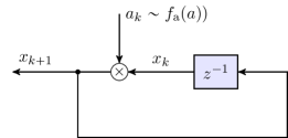
Figure 1: Process dynamics. The upper system generating the stochastic dynamics is shown as a multiplicative noise signal in a feedback loop. The equivalent system below is a feedback loop with a stochastic gain.

This is the simplest case of the type of processes described above. As we are considering only a scalar state and uncorrelated $a_{k}$ it is too simplistic for many real processes of this type. However, it is a prototypical case and illustrates some of the phenomena that may arise in more complex systems. Understanding the stability characteristics of this system is a precursor to understanding those for more complex systems.

II-A Stability

At the time index $K$ the state $x_{K}$ is given by

$$x_{K}=\prod_{k=0}^{K-1}a_{k}\,x_{0},$$

and as $a_{k}\sim f_{\text{a}}\!\left(a\right)$ the state $x_{K}$ is also a stochastic variable with a probability density function we denote by $f_{\text{x}_{K}}\!\left(x\right)$. We are interested in the properties of this distribution as $K\longrightarrow\infty$. More specifically we will derive conditions for the following three notions of stability.

The system is defined as median stable if and only if

$$\lim_{K\longrightarrow\infty}\,\operatorname{median}(x_{K})\,=\,0.$$

The system is defined as mean stable if and only if

$$\lim_{K\longrightarrow\infty}\,{\cal E}\left[\rule{0.0pt}{8.99994pt}x_{K}\right]\,=\,0,$$

and the system is defined as variance stable if and only if

$$\lim_{K\longrightarrow\infty}\,{\cal E}\left[\rule{0.0pt}{8.99994pt}(x_{K}-E\{x_{K}\})^{2}\right]\,=\,0.$$

The approach taken will involve analysing the system in terms of the probability density functions of the logarithmic variables,

$$\zeta_{k}:=g(x_{k})=\ln(x_{k})$$ (5)

and

$$\alpha_{k}:=g(a_{k})=\ln(a_{k}).$$ (6)

The function $g$ is defined here for convenience in subsequent derivations.

We will assume that $x_{0}>0$ is given and so $x_{K}\geq 0$ for all $K\in{\mathbbm{Z}}_{+}$. For simplicity in the following we will assume without loss of generality that $x_{0}=1$. The evolution of the dynamics in (4) now becomes

$$\zeta_{k+1}=\zeta_{k}+\alpha_{k}.$$ (7)

This allows us to express $x_{K}$ as,

$$x_{K}\;=\;\text{e}^{\zeta_{K}}$$

To illustrate the way in which stability results will be derived we can examine this evolution for $K$ timesteps. Under our assumption that $x_{0}=1$,

$${\cal E}\left[\rule{0.0pt}{8.99994pt}\zeta_{K}\right]={\cal E}\left[\rule{0.0pt}{8.99994pt}\sum_{k=0}^{K-1}\alpha_{k}\right]=K{\cal E}\left[\rule{0.0pt}{8.99994pt}\alpha\right]=K\mu_{\alpha},$$

if the distributions $f_{\alpha_{k}}\!\left(\alpha\right)$ are identically distributed.

It is tempting to say that if $\mu_{\alpha}<0$ then ${\cal E}\left[\rule{0.0pt}{8.99994pt}x_{K}\right]<1$. This is not true as the results in the following sections will make clear. What will turn out to be true is that for distributions where the distribution of $\ln(a)$ satisfies certain moment assumptions,

$${\cal E}\left[\rule{0.0pt}{8.99994pt}\alpha\right]\,<\,0\quad\iff\quad\lim_{K\longrightarrow\infty}\operatorname{median}(x_{K})\,=\,0.$$

II-B Commutative variable relationships

The system will be studied in terms of the probability distributions of both the $x_{k}$, $a_{k}$ variables and their logarithmic versions, $\zeta_{k}$, $\alpha_{k}$. The logarithmic/exponential relationship between these variables means that one can map the distributions from one set of variables to the other. Figure 2 gives a commutative diagram of these relationships as they evolve over the time index.

Figure 2: State variable evolution. The mapping between the $x$ and $\zeta$ variables is given by $\zeta_{i}=g(x_{i})=\ln(x_{i})$, and the inverse mapping is $x_{i}=g^{-1}(\zeta_{i})=\text{e}^{\zeta_{i}}.$

The mappings to logarithmic variables in (5) and (6) maps the corresponding distributions. This is described for the $\alpha$ variable but also applies to the $x_{k}$ variables. Suppose that $a$ has a probability distribution $f_{\text{a}}\!\left(a\right)$ defined on a support $S_{\text{a}}\subseteq{\mathbbm{R}}_{+}$,

$$S_{\text{a}}=\left\{a\,\mid\,f_{\text{a}}\!\left(a\right)>0\right\}.$$

If $g(a)$ is monotonically increasing and invertible on $S_{\text{a}}$ then the probability distribution of $\alpha$ is given by,

$$f_{\alpha}\!\left(\alpha\right)=\left\{\begin{array}[]{ll}f_{\text{a}}\!\left(g^{-1}(\alpha)\right)\displaystyle\left|\frac{\mathop{}\!\mathrm{d}\,g^{-1}(\alpha)}{\mathop{}\!\mathrm{d}\alpha}\right|,&\text{if }\alpha\in S_{\alpha},\\ 0,&\text{if }\alpha\notin S_{\alpha}.\end{array}\right.$$ (8)

and has support,

$$S_{\alpha}=\left\{\alpha=g(a)\,\mid\,a\in S_{\text{a}}\right\}.$$

In our case

$$g(a)=\ln(a),\quad g^{-1}(\alpha)=\text{e}^{\alpha},$$

and

$$\left|\frac{\mathop{}\!\mathrm{d}\,g^{-1}(\alpha)}{\mathop{}\!\mathrm{d}\alpha}\right|=\left|\text{e}^{\alpha}\right|=\text{e}^{\alpha}.$$

We are interested in the distribution of $x_{K}$ as $K$ increases and, as we can see from Figure 2, there are several ways of calculating this distribution. One can directly consider the evolution of the variable,

$$x_{k+1}\>=\>a_{k}\,x_{k},$$

where $x_{k}$ has density $f_{\text{x}_{k}}\!\left(x\right)$ and $a_{k}$ has density $f_{\text{a}}\!\left(a\right)$. This can be calculated as,

$$f_{\text{x}_{k+1}}\!\left(x\right)=\int_{-\infty}^{\infty}f_{\text{x}_{k}}\!\left(\xi\right)f_{\text{a}}\!\left(x/\xi\right)\frac{1}{|\xi|}\mathop{}\!\mathrm{d}\xi.$$

The $f_{\text{x}_{k+1}}\!\left(x\right)$ distribution can also be obtained by first transforming $x_{k}$ to $\zeta_{k}$ using the mapping in (8),

$$f_{\zeta_{k}}\!\left(\zeta\right)=f_{\text{x}_{k}}\!\left(\text{e}^{\zeta}\right)\text{e}^{\zeta}.$$

The $\zeta$ dynamics are simply additive (see (7)) and so the $\zeta_{k+1}$ distribution is given by the convolution,

$$f_{\zeta_{k+1}}\!\left(\zeta\right)=\int_{-\infty}^{\infty}f_{\zeta_{k}}\!\left(\xi\right)f_{\text{a}}\!\left(\zeta-\xi\right)\mathop{}\!\mathrm{d}\xi.$$

The $f_{\text{x}_{k+1}}\!\left(x\right)$ distribution is then given by the inverse of the mapping in (8),

$$f_{\text{x}_{k+1}}\!\left(x\right)=f_{\zeta_{k+1}}\!\left(\ln(x)\right)\frac{1}{x},\quad x>0.$$

II-C Lognormal distributions

The case where $f_{\text{a}}\!\left(a\right)$ is a lognormal distribution is in some sense generic. If $f_{\text{a}}\!\left(a\right)$ is a lognormal distribution, then $f_{\alpha}\!\left(\alpha\right)$ is normal. Then the $\zeta_{K}$ distribution is a sum of normal distributions and is also normal. Equivalently the distribution of $x_{K}$ is lognormal for all $K$. In other words, lognormal distributions are closed under multiplication of the random variables.

The central limit theorem implies that even if the $f_{\alpha}\!\left(\alpha\right)$ distribution is not normal, the scaled distribution of $\zeta_{K}$ tends to a normal distribution. One therefore also expects that the scaled $x_{K}$ distribution tends to a lognormal distribution. We present some of the properties of lognormal distributions for later use. All of the results here can be found in [21].

The lognormal distribution can be defined by considering $a$ as given by,

$$a=\text{e}^{\alpha}\quad\text{where}\quad\alpha\;\sim\;{\cal N}(\mu_{\alpha},\sigma^{2}_{\alpha}).$$

The parameters $\mu_{\alpha}$ and $\sigma_{\alpha}$ are known as the location and scale parameters respectively, but here we simply refer to them as the mean and standard deviation in the $\alpha$-space. This distribution definition ensures that $S_{\text{a}}={\mathbbm{R}}_{+}$ and so fits the assumptions of our problem.

From (7) it is clear that $\zeta_{K}$ is the sum of $K$ random variables, $\alpha_{k}$, with each $\alpha_{k}\sim{\cal N}(\mu_{\alpha},\sigma^{2}_{\alpha})$. The sum of normally distributed variable is also normally distributed and

$$\zeta_{K}\,\sim\,{\cal N}(K\mu_{\alpha},K\sigma^{2}_{\alpha}).$$

This gives a closed-form expression for the distribution of $\zeta_{K}$,

$$f_{\zeta_{K}}\!\left(\zeta\right)=f_{\cal N}\!\left(\alpha,K\mu_{\alpha},K\sigma^{2}_{\alpha}\right),$$ (9)

where

$$f_{\cal N}\!\left(x,\mu,\sigma^{2}\right)=\frac{1}{\sqrt{2\pi\sigma^{2}}}\text{e}^{-(x-\mu)^{2}/2\sigma^{2}}.$$

Closed-form expressions relate the mean and variance of $a_{k}$ to the mean and variance of $\alpha_{k}$ [22, 23].

$$\mu_{\alpha} = \ln\left(\frac{\mu_{a}}{\sqrt{1+\frac{\sigma_{a}^{2}}{\mu_{a}^{2}}}}\right)$$ (10)

$$\sigma_{\alpha}^{2} = \ln\left(1+\frac{\sigma_{a}^{2}}{\mu_{a}^{2}}\right).$$ (11)

The inverse mapping is given by,

$$\mu_{a} = \text{e}^{\mu_{\alpha}+\sigma_{\alpha}^{2}/2}$$ (12)

$$\sigma_{a}^{2} = \left(\text{e}^{\sigma_{\alpha}^{2}}-1\right)\left(\text{e}^{2\mu_{\alpha}+\sigma_{\alpha}^{2}}\right).$$ (13)

The fact that the mean and variance of $a$ are not simply the exponentiation of the corresponding $\alpha$ domain values leads to interesting characterisations of stability in the $x$ domain.

The mode and median of $a$ are also given by simple expressions,

$$\operatorname{mode}(a) = \text{e}^{\mu_{\alpha}-\sigma_{\alpha}^{2}}$$ (14)

$$\operatorname{median}(a) = \text{e}^{\mu_{\alpha}}.$$ (15)

The median condition—and any other quantile value—is transformed via exponentiation making it a simple matter to characterise properties of the median or quantile value.

III Stability conditions

The following sections derive the conditions under which the median, mean, and variance of $f_{\text{x}_{K}}\!\left(x\right)$ converge to zero as $K\longrightarrow\infty$.

III-A Mean stability

The condition for the stability of the mean of $x_{K}$ is a simple consequence of the fact that for two independent distributions, the product of the expectations is equal to the expectation of the product.

Theorem 1 (Mean stability)

$$\lim_{K\longrightarrow\infty}\operatorname{mean}(x_{K})\,=\,0\quad\iff\quad\mu_{a}<1.$$

For lognormal distributions (12) shows that the mean stability condition can also be stated in terms in the mean and variance of the $f_{\alpha}\!\left(\alpha\right)$ distribution,

$$\lim_{K\longrightarrow\infty}\operatorname{mean}(x_{K})\,=\,0\quad\iff\quad\mu_{\alpha}+\sigma_{\alpha}^{2}/2\,<\,0.$$

III-B Variance stability

Goodman [24] derives the variance of a product of arbitrary distributions which directly leads to the following variance stability result.

Theorem 2 (Variance stability)

$$\lim_{K\longrightarrow\infty}\operatorname{variance}(x_{K})\,=\,0\quad\iff\quad\mu_{a}^{2}+\sigma_{a}^{2}<1.$$

Proof:

From [24] we have ,

$$\operatorname{variance}(x_{K}) = \operatorname{variance}\left(\prod_{k=0}^{K-1}a_{k}\right)$$

$$= \prod_{k=0}^{K-1}\left(\sigma_{a}^{2}+\mu_{a}^{2}\right)-\prod_{k=0}^{K-1}\mu_{a}^{2},$$

which in our i.i.d. case gives,

$$\operatorname{variance}(x_{K}) = \left(\sigma_{a}^{2}+\mu_{a}^{2}\right)^{K}-\mu_{a}^{2K}$$ (17)

$$= \sigma_{a}^{2}(\sigma_{a}^{2}+\mu_{a}^{2})^{K-1}$$

$$+\>\mu_{a}^{2K}\left(\left(1+\frac{\sigma_{a}^{2}}{\mu_{a}^{2}}\right)^{K-1}-1\right).$$

If $\sigma_{a}^{2}+\mu_{a}^{2}<1$ then both terms in (17) go to zero as $K\longrightarrow\infty$. In the case where $\sigma_{a}^{2}+\mu_{a}^{2}=1$ and $\sigma_{a}^{2}>0$ (17) also shows that the variance of $x_{K}$ goes to one as $K\longrightarrow\infty$. If $\sigma_{a}^{2}+\mu_{a}^{2}>1$ then both terms in (17) grow without bound as $K\longrightarrow\infty$. ∎

In the lognormal distribution case, substituting (12) and (13) into the condition of Theorem 2 gives an equivalent condition in terms of the normal $f_{\alpha}\!\left(\alpha\right)$ distribution.

$$\lim_{K\longrightarrow\infty}\operatorname{variance}(x_{K})\,=\,0\quad\iff\quad\mu_{\alpha}+\sigma_{\alpha}^{2}<0.$$

III-C Median stability: lognormal case

The least restrictive stability condition to be considered is that for the median of $x_{K}$. This result is easy to obtain for a lognormal distribution and so we do that first.

Theorem 3 (Median stability; lognormal distribution)

If $f_{\text{a}}\!\left(a\right)$ is a lognormal distribution,

$$\lim_{K\longrightarrow\infty}\operatorname{median}(x_{K})\,=\,0\quad\iff\quad\mu_{\alpha}<0.$$

Proof:

As $f_{\zeta_{K}}\!\left(x\right)$ is a normal distribution its median is equal to its mean,

$$\operatorname{median}(\zeta_{k})=\operatorname{mean}(\zeta_{K})=K\mu_{\alpha}.$$

This immediately gives $\lim_{K\longrightarrow\infty}\operatorname{median}(\zeta_{K})=-\infty$ if and only if $\mu_{\alpha}<0$. As $\operatorname{median}(x_{k})=\text{e}^{\operatorname{median}(\zeta_{K})}$ the result follows. ∎

From (10) we can also express the condition of Theorem 3 in terms of the $f_{\text{a}}\!\left(a\right)$ distribution,

$$\lim_{K\longrightarrow\infty}\operatorname{median}(x_{K})\,=\,0\quad\iff\quad\mu_{a}^{2}-\frac{\sigma_{a}^{2}}{\mu_{a}^{2}}<1.$$

Note that, depending on the variance $\sigma^{2}_{a}$, systems with mean $\mu_{a}$ greater than one might still be median stable. This point will be discussed in greater detail later.

The stability results for lognormal distributions are summarised in Table I. All of the conditions can be expressed in terms of the mean and variances of both the $f_{\text{a}}\!\left(a\right)$ and the $f_{\alpha}\!\left(\alpha\right)$ distributions.

Stability property	$f_{\text{a}}\!\left(a\right)$ distribution	$f_{\alpha}\!\left(\alpha\right)$ distribution
$\operatorname{median}(x_{K})$	$\mu_{a}^{2}-\sigma_{a}^{2}/\mu_{a}^{2}<1$	$\mu_{\alpha}<0$
$\operatorname{mean}(x_{K})$	$\mu_{a}<1$	$\mu_{\alpha}+\sigma_{\alpha}^{2}/2<0$
$\operatorname{variance}(x_{K})$	$\mu_{a}^{2}+\sigma_{a}^{2}<1$	$\mu_{\alpha}+\sigma_{\alpha}^{2}<0$

TABLE I: Stochastic feedback gain stability conditions for lognormal distributions

III-D Median stability: general distributions

We now consider median stability in the case where the $f_{\text{a}}\!\left(a\right)$ distributions are other than lognormal. The mean and variance relationships between the $f_{\text{a}}\!\left(a\right)$ and $f_{\alpha}\!\left(\alpha\right)$ distributions given in Equations (10) to (13) no longer hold. Unfortunately this is also true for all values of $K$ and also in the limit as $K\longrightarrow\infty$.

The situation is more complex for more general $f_{\text{a}}\!\left(a\right)$ distributions as $f_{\alpha}\!\left(\alpha\right)$ is not normal. In the context of the central limit theorem, it is perhaps surprising that although the distribution $f_{\zeta_{K}}\!\left(\zeta\right)$ is the $K$-fold convolution of the $f_{\alpha}\!\left(\alpha\right)$ distributions, the median of $f_{\zeta_{K}}\!\left(\zeta\right)$ does not necessarily converge to the mean of $f_{\zeta_{K}}\!\left(\zeta\right)$. The difference can be quantified.

Lemma 4

Assume that $f_{\alpha}\!\left(\alpha\right)$ is a non-lattice distribution with bounded third moment. Then

$$\lim_{K\longrightarrow\infty}\>\operatorname{median}(\zeta_{K})\,-\,{\cal E}\left[\rule{0.0pt}{8.99994pt}\zeta_{K}\right]\>=\>-\frac{{\cal E}\left[\rule{0.0pt}{8.99994pt}(\alpha-\mu_{\alpha})^{3}\right]}{6\sigma_{\alpha}^{2}}.$$

A lattice distribution is one where there exist parameters $b\in{\mathbbm{R}}$ and $h>0$ such that $\operatorname{Prob}\{\alpha\in b+h{\mathbbm{Z}}\}=1.$

Proof:

$$\operatorname{median}(\zeta_{K})-{\cal E}\left[\rule{0.0pt}{8.99994pt}\zeta_{K}\right] = \operatorname{median}\left(\sum_{k=0}^{K-1}\alpha\right)-K\mu_{\alpha}$$

$$= \sigma_{\alpha}\operatorname{median}\left(\sum_{k=0}^{K-1}\frac{\alpha-\mu_{\alpha}}{\sigma_{\alpha}}\right).$$

Define a new stochastic variable $y$ with probability density function $f_{y}(y)$ by,

$$y:=h(\alpha)=\frac{\alpha-\mu_{\alpha}}{\sigma_{\alpha}},$$

and note that ${\cal E}\left[\rule{0.0pt}{8.99994pt}y\right]=\mu_{y}=0$ and ${\cal E}\left[\rule{0.0pt}{8.99994pt}y^{2}\right]=\sigma_{y}^{2}=1$. Define $\tau$ as the third moment of $f_{y}(y)$,

$$\tau:={\cal E}\left[\rule{0.0pt}{8.99994pt}y^{3}\right],$$

and by assumption $\tau<\infty$. The following result is from Hall [25] provides the key step. If $f_{y}(y)$ is a non-lattice distribution with $\mu_{y}=0$, $\sigma_{y}=1$ and ${\cal E}\left[\rule{0.0pt}{8.99994pt}y^{3}\right]=\tau<\infty$, then,

$$\lim_{K\longrightarrow\infty}\operatorname{median}\left(\sum_{k=0}^{K-1}y\right)\>=\>\frac{-\tau}{6}.$$

As

$$\IEEEeqnarraymulticol{3}{l}{\lim_{K\longrightarrow\infty}\>\operatorname{median}(\zeta_{K})\,-\,{\cal E}\left[\rule{0.0pt}{8.99994pt}\zeta_{K}\right]}$$

$$= \sigma_{\alpha}\operatorname{median}\left(\sum_{k=0}^{K-1}\frac{\alpha-\mu_{\alpha}}{\sigma_{\alpha}}\right)$$ (18)

$$= \sigma_{\alpha}\operatorname{median}\left(\sum_{k=0}^{K-1}y\right)\>=\>\frac{-\sigma_{\alpha}\,\tau}{6},$$

it only remains to determine the value of $\tau$. As $h^{-1}(y)=\sigma_{\alpha}y+\mu_{\alpha}$,

$$\tau = \int_{-\infty}^{\infty}y^{3}f_{y}(y)\mathop{}\!\mathrm{d}y$$

$$= \int_{-\infty}^{\infty}y^{3}f_{\alpha}\!\left(h^{-1}(y)\right)\left|\frac{dh^{-1}(y)}{dy}\right|\,\mathop{}\!\mathrm{d}y$$

$$= \int_{-\infty}^{\infty}y^{3}f_{\alpha}\!\left(\sigma_{\alpha}y+\mu_{\alpha}\right)|\sigma_{\alpha}|\,\mathop{}\!\mathrm{d}y$$

$$= \int_{-\infty}^{\infty}\frac{(\alpha-\mu_{\alpha})^{3}}{\sigma_{\alpha}^{3}}f_{\alpha}\!\left(\alpha\right)|\sigma_{\alpha}|\,\frac{\mathop{}\!\mathrm{d}\alpha}{|\sigma_{\alpha}|}$$

$$= \frac{1}{\sigma_{\alpha}^{3}}\int_{-\infty}^{\infty}(\alpha-\mu_{\alpha})^{3}f_{\alpha}\!\left(\alpha\right)\mathop{}\!\mathrm{d}\alpha$$

$$= \frac{{\cal E}\left[\rule{0.0pt}{8.99994pt}(\alpha-\mu_{\alpha})^{3}\right]}{\sigma_{\alpha}^{3}}.$$

Substituting the above into (18) gives the desired result. ∎

The key point in determining the median stability is that the limit in Lemma 4 is independent of $K$.

Theorem 5 (Median stability))

Assume that $f_{\alpha}\!\left(\alpha\right)$ is a nonlattice distribution with bounded third moment. Then,

$$\lim_{K\longrightarrow\infty}\operatorname{median}(x_{K})\;=\;0\quad\iff\quad\mu_{\alpha}\;<\;0.$$

Proof:

If $\mu_{\alpha}=0$ then ${\cal E}\left[\rule{0.0pt}{8.99994pt}\zeta_{K}\right]\;=\;K\mu_{\alpha}\;=\;0$, and from Lemma 4, $\lim_{K\longrightarrow\infty}\operatorname{median}(\zeta_{K})$ is a finite constant. Therefore,

$$\lim_{K\longrightarrow\infty}\operatorname{median}(x_{K})\;=\;\lim_{K\longrightarrow\infty}\text{e}^{\operatorname{median}(\zeta_{K})}\;\neq\;0.$$

By Lemma 4, for every $\epsilon>0$, there exists an integer $\bar{K}$ such that for all $K>\bar{K}$,

$$\left|\operatorname{median}(\zeta_{K})-K\mu_{\alpha}+\frac{{\cal E}\left[\rule{0.0pt}{8.99994pt}(\alpha-\mu_{\alpha})^{3}\right]}{6\sigma_{\alpha}^{2}}\right|\><\>\epsilon.$$

This implies that

$$|\operatorname{median}(\zeta_{K})-K\mu_{\alpha}|\><\>\left|\frac{{\cal E}\left[\rule{0.0pt}{8.99994pt}(\alpha-\mu_{\alpha})^{3}\right]}{6\sigma_{\alpha}^{2}}\right|\,+\,\epsilon.$$

If we now assume that $\mu_{\alpha}<0$ then $K\mu_{\alpha}<0$ and

$$\operatorname{median}(\zeta_{K})\><\>K\mu_{\alpha}+\left|\frac{{\cal E}\left[\rule{0.0pt}{8.99994pt}(\alpha-\mu_{\alpha})^{3}\right]}{6\,\sigma_{\alpha}^{2}}\right|\,+\,\epsilon.$$

The righthand side clearly goes to $-\infty$ as $K\longrightarrow\infty$. An analogous argument for $\mu_{\alpha}>0$ gives a lower bound on $\operatorname{median}(\zeta_{K})$ that goes to $\infty$ as $K\longrightarrow\infty$. Exponentiating $\operatorname{median}(\zeta_{K})$ gives the required result. ∎

This result also follows from Cantelli’s inequality (see Lemma 8) without the requirement of a bounded third moment. However the method of proof above illustrates the manner in which a sum of non-normal distributions does not converge to a normal distribution. It also gives the following interesting boundary condition.

Corollary 6 (Median limit: zero mean log distribution)

If $f_{\alpha}\!\left(\alpha\right)$ is a non-lattice distribution with $\mu_{\alpha}=0$ and $\left|{\cal E}\left[\rule{0.0pt}{8.99994pt}(\alpha-\mu_{\alpha})^{3}\right]\right|<\infty$ then,

$$\lim_{K\longrightarrow\infty}\operatorname{median}(x_{K})\>=\>\text{e}^{\displaystyle-\frac{{\cal E}\left[\rule{0.0pt}{8.99994pt}(\alpha-\mu_{\alpha})^{3}\right]}{6\,\sigma_{\alpha}^{2}}}.$$

Ethier [7] also uses the result of Hall to prove a similar result on the median of a gambler’s fortune. The results in [7] suggest that the assumption of a non-lattice distribution in Lemma 4 may be able to be removed. Such distributions are important for gambling applications but may be of less interest in many control applications.

The stability conditions for more general distributions (non-lattice and with bounded third moment) are summarised in Table II.

Stability property	$f_{\text{a}}\!\left(a\right)$ distribution	$f_{\alpha}\!\left(\alpha\right)$ distribution
$\operatorname{median}(x_{K})$	—	$\mu_{\alpha}<0$
$\operatorname{mean}(x_{K})$	$\mu_{a}<1$	—
$\operatorname{variance}(x_{K})$	$\mu_{a}^{2}+\sigma_{a}^{2}<1$	—

TABLE II: Stochastic feedback gain stability conditions for more general distributions

The median stability conditions given here for a stochastic gain $a_{k}\sim f_{\text{a}}\!\left(a\right)$ have a similar form to the stability conditions for a time-varying gain. Section III-E gives more detail on this perspective.

III-E Stabilisation by time-varying gains and the geometric mean

Some of the initially unintuitive phenomena observed for stochastic feedback may be better understood by considering systems with certain types of deterministic, but time-varying feedback gains. For the case of a scalar state, a complete analysis is easy to do. For a more complete analysis of the periodic multivariable case see for example [26]. Consider the single-state discrete-time system and its solution

$$x_{k+1}~{}=~{}a_{k}~{}x_{k}\quad\Longrightarrow\quad x_{K}~{}=~{}\left(\prod_{k=0}^{K-1}a_{k}\right)x_{0}.$$ (19)

If $a$ is a periodic signal with period $N$, then the growth of $x$ can be characterised by observing the behaviour every $N$ time steps. Define the “sub-sampled state”

$$\hat{x}_{k}~{}:=~{}x_{kN}.$$

Note that $x$ decays iff $\hat{x}$ decays since the growth of $x$ in between the subsamples is bounded. The recursion for $\hat{x}$ is time invariant

$$\hat{x}_{k+1}~{}=~{}x_{(k+1)N}~{}=~{}\left(\prod_{k=0}^{N-1}a(k)\right)x_{kN}~{}=:~{}\hat{a}~{}\hat{x}_{k},$$

where $\hat{a}:=\prod_{k=0}^{N-1}a_{k}$ is the so-called “monodromy gain”. Thus the sequence $\hat{x}$ decays iff

$$|\hat{a}|<1\quad\Leftrightarrow\quad|\hat{a}|^{\frac{1}{N}}<1\quad\Leftrightarrow\quad\left(\prod_{k=0}^{N-1}|a_{k}|\right)^{\frac{1}{N}}<1.$$ (20)

The last quantity in (20) is the geometric mean of the absolute value of the signal $a$, which is the right quantity that characterises stability in this system. The geometric mean can also be expressed using the arithmetic mean of the logarithm,

$$\left(\prod_{k=0}^{N-1}|a_{k}|\right)^{\frac{1}{N}}<1\quad \Leftrightarrow \quad\ln\left(\prod_{k=0}^{N-1}|a_{k}|\right)^{\frac{1}{N}}\!\!\!\!<\,0$$

$$\Leftrightarrow \quad\frac{1}{N}\sum_{k=0}^{N-1}\ln\big{|}a_{k}\big{|}~{}<~{}0.$$

Thus the system is asymptotically stable iff the arithmetic mean of $\left\{\ln|a_{k}|\right\}$ is negative. Note how this is analogous to the condition $E\{\ln|a|\}<0$ when $a$ is a stochastic process. The relation between the geometric mean and the arithmetic mean through the logarithm function is illustrated in Figure 3. The figure illustrates a periodic gain $a$ that is symmetrically distributed around 1. The $\ln(a_{k})$ mapping tends to boost values of $\{a_{k}\}$ that are less than 1 more heavily towards large negative numbers while tempering the values of $\{a_{k}\}$ that are larger than 1 by mapping them to smaller positive numbers. The result is that even though $a$ maybe symmetrically distributed around 1, the product $\prod_{k=0}^{N-1}\left|a_{k}\right|$ will be strictly smaller than 1.

Figure 3: An illustration of the mapping from $a_{k}$ to $\ln|a_{k}|$ showing that when $a$ is symmetrically distributed around $1$, $\ln|a|$ is distributed more heavily towards negative numbers due to the distortion by the $\ln$ mapping. The cyan dashed line on the graph of $\ln|a|$ indicates the arithmetic mean of that signal (this is the logarithm of the geometric mean of $a$) showing how it is negative while the $\ln$ of the mean of $a$ is zero.

Now let’s examine (19) in the case where the sequence $\{a_{k}\}$ is a general time-varying gain. The asymptotic behavior of the solution is completely determined by the limit of the product of the gains $\{a_{k}\}$, which can be studied as a series limit by taking the logarithm,

$$\ln\left|\prod_{k=0}^{K-1}a_{k}\right|~{}=~{}\sum_{k=0}^{K-1}\ln\big{|}a_{k}\big{|}.$$

Now explore the limit

$$\lim_{K\rightarrow\infty}\sum_{k=0}^{K-1}\ln\big{|}a_{k}\big{|} = \lim_{K\rightarrow\infty}~{}K\left(\frac{1}{K}\sum_{k=0}^{K-1}\ln\big{|}a_{k}\big{|}\right)$$

$$= K\left(\lim_{K\rightarrow\infty}~{}\frac{1}{K}\sum_{k=0}^{K-1}\ln\big{|}a_{k}\big{|}\right)$$

$$=: K~{}{\cal E}\left[\ln|a|\right],$$

where the last limit is expressed in terms of the asymptotic average, which for any signal $u$ is defined by

$${\cal E}\left[u\right]:=\lim_{K\rightarrow\infty}\frac{1}{K}\sum_{k=0}^{K-1}u_{k}.$$

This asymptotic average can be thought of as a “deterministic expectation” of $u$, which is equivalently the time average of a realization of a stochastic process.

We can thus conclude that if the asymptotic average of $\ln|a|$ exists and is negative, then the state will asymptotically converge to zero, i.e.

$${\cal E}\left[\rule{0.0pt}{8.99994pt}\ln\left|a\right|\right]~{}<~{}0\quad\Rightarrow\quad\lim_{K\rightarrow\infty}x_{K}~{}=~{}0.$$ (21)

We can actually conclude something slightly stronger,

$${\cal E}\left[\rule{0.0pt}{8.99994pt}\ln|a|\right]~{}=:~{}\ln(\gamma)~{}<~{}0\quad\Rightarrow\quad\left|x_{K}\right|~{}\leq~{}\alpha~{}\gamma^{K},$$ (22)

i.e. the convergence is geometric with decay rate $\gamma<1$. Finally we note that condition (22) is only necessary for exponential convergence. Slower convergence can still occur even when this condition does not hold. For convergence we simply need the sequence on the right hand side of (III-E) to go to $-\infty$. This can occur even when the asymptotic average is converging to zero (from below), as long as it converges at a rate slower than $1/K$. More precisely we can state

$$\lim_{K\rightarrow\infty}x_{K}=0\\ \Leftrightarrow\quad\lim_{K\rightarrow\infty}~{}K\left(\frac{1}{K}\sum_{k=0}^{K-1}\ln\big{|}a_{k}\big{|}\right)=-\infty.$$

III-F Stability regions

The variance, mean, and median stability regions for the $f_{\text{a}}\!\left(a\right)$ distribution are shown in Figure 4. The most interesting observation is that there exists a region in which $\operatorname{median}(x_{K}$) is stable and the $\operatorname{mean}(x_{K})$ is unstable. We will subsequently show (in Section IV) that in this case the sample paths $x_{K}$ go to zero almost surely but the mean of $x_{K}$ goes to $\infty$. This analysis can also be applied to other feedback loops and Section III-G derives the stability regions for a first order system with unknown gain and pole position.

Figure 4: Stability regions in the $a$ domain. The region where the condition is satisfied is to the left of the correspondingly coloured boundary. The mean and variance stability regions are applicable to general distributions. The median stability region shown here applies to lognormal $f_{\text{a}}\!\left(a\right)$ distributions. Other distributions will have slightly different median stability regions, but identical mean and variance stability regions. The four circles indicate the values of $\mu_{\alpha}$ and $\sigma_{\alpha}$ of the distributions shown in Figure 5.

Figure 5 gives the probability distribution functions for four stability cases: unstable, median stable, mean stable, and variance stable. In all cases the mode of the distribution is less than one. The remarkable feature of these distributions is that they are not particularly different and yet give very different stability characteristics in the evolution of the state.

Figure 5: Probability density functions of $a$ for four stability cases: variance stable, mean stable, median stable, and unstable. All four cases have the same mode; their means and standard deviations are shown in Figure 4.

The most intriguing case is that where the median of $x_{K}$ is stable, but the mean is unstable. Figure 6 shows the evolution of the log-normal probability density function of $x_{K}$ for a range of values of $K$. The evolution of the median towards zero, and the mean towards infinity, are clear in the distributions.

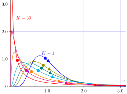
Figure 6: Evolution of the probability density function of $x_{K}$ for $K=1,2,3,5,10,15$, and $30$. The mean values of each $x_{K}$ distribution are indicated by triangles and the median values are indicated by solid dots. As $K\longrightarrow\infty$ the mean of $x_{K}$ increases and the median decreases.

We illustrate the median stable/mean unstable case by simulating 200 sample paths. The $f_{\text{a}}\!\left(a\right)$ distribution is the lognormal distribution with probability density function shown as Case 3 of Figure 5 ($\mu_{a}=1.0283$, $\sigma_{a}=0.4389$). Figure 7 illustrates the sample paths and the evolution of the distribution, $f_{\alpha}\!\left(\alpha\right)$. As $K$ increases the median stability condition ensures that the sample paths go to zero almost surely. However $\mu_{a}>1$ and so the $\operatorname{mean}(x_{K})$ is unstable and goes to $\infty$. For $K$ very large this results in an $x_{K}$ distribution with a very high peak close to $x_{K}=0$, but still having enough weight in the positive tail that the mean of $x_{K}$ is very large (and growing with $K$). The sample estimate of $\operatorname{mean}(x_{K})$ (denoted by $\hat{\mu}_{x_{K}}$) drops below the theoretical mean, $\mu_{x_{K}}$ as increasingly fewer sample paths are near or above the mean. This phenomenon is investigated in more detail in Section IV.

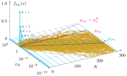
Figure 7: Simulation of the median stable/mean unstable case. The vertical axis shows the evolution of the probability density function, $f_{x_{K}}(x)$ for a range of values of $K$. The horizontal plane shows 200 simulation sample paths of $x_{K}$ as a function of $K$. Also shown are the sample median (blue line) and sample mean (red line: $\hat{\mu}_{x_{K}}$), along with the theoretical median (cyan line: $\text{e}^{K\mu_{\alpha}}$) and theoretical mean (magenta line: $\mu_{x_{K}}$). The theoretical values are derived by mapping the $\alpha$-space distribution in (9) through the equations (15) and (14).

III-G Stochastic gain stabilisation

The stability results for stochastic feedback can easily be applied to the slightly more problem of stabilising a general first order system via stochastic feedback. Figure 8 illustrates the configuration for this problem. This is a simple case of a more general stochastic stabilisation problem, referred to as stabilisation by noise. This problem has been studied in stochastic vibration control context (see the review [27]). In vibration control the assumption of an oscillatory nominal response is usually exploited. The more general case is studied in [28] and is based on earlier work in [29]. This work focuses the continuous-time equivalent to the mean stability case considered in this paper. The application example given here has also been studied in [13], where a result which is essentially equivalent to the median stability boundary below is presented.

Figure 8: Stochastic stabilisation problem. A first order plant is connected in feedback with a stochastic gain $\delta_{k}\sim f_{\delta}\!\left(\delta\right)$.

The plant is given and has the transfer function $G(z)$,

$$G(z)\>=\>\frac{\gamma}{z-\tau}.$$

Denote the plant output by $y_{k}$. The closed loop dynamics of the feedback system illustrated in Figure 8 are given by,

$$y_{k+1}\>=\>\left(\tau+\gamma\delta_{k}\right)\,y_{k},$$

where $\delta_{k}\sim f_{\delta}\!\left(\delta\right)$ is the stochastic feedback drawn from a known distribution at each time instant.

Now define $x_{k}$ = $|y_{k}|$ and note that,

$$x_{k+1}\>=\>|\tau+\gamma\delta_{k}|\,x_{k}.$$

As $x_{k}\geq 0$ for all $k$, the results summarised in Table II are directly applicable by defining

$$a_{k}\>=\>|\tau+\gamma\delta_{k}|.$$

The mean of the $f_{\text{a}}\!\left(a\right)$ distribution is,

$$\mu_{a}\>=\>|\tau+\gamma\mu_{\delta}|.$$

The variance may be more difficult to evaluate precisely but can be easily estimated numerically. If the distribution $f_{\delta}\!\left(\delta\right)$ were such that $\delta_{k}>0$ then,

$$\sigma^{2}_{a}\;=\;\gamma\sigma^{2}_{\delta}.$$

However the absolute value in the definition of $a$ complicates this somewhat, particularly in the case of interest where $\tau\neq 0$.

As expected the conditions for median, mean, and variance stability differ and for a given distribution, $f_{\delta}\!\left(\delta\right)$, a stability boundary diagram, analogous to that in Figure 4, can be drawn. Figure 9 illustrates the stability regions for the case where $\delta_{k}$ is drawn from a normal distribution, $\delta_{k}\sim{\cal N}(\mu_{\delta},\sigma^{2}_{\delta})$.

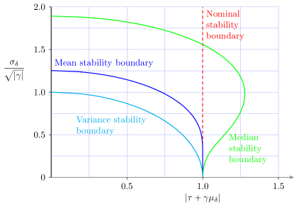
Figure 9: Stability boundaries for the state-magnitude evolution for the plant, $G(z)=\gamma/(z-\tau)$, in feedback with a stochastic gain, $\delta_{k}\sim{\cal N}(\mu_{\delta},\sigma^{2}_{\delta})$. Unstable open-loop plants may be median stabilised by a stochastic gain with the appropriate mean and variance.

An $f_{\delta}\!\left(\delta\right)$ distribution with a non-zero mean can be viewed as a constant feedback gain of $\mu_{\delta}$ in parallel with a zero-mean stochastic gain. The static feedback effect of $\mu_{\delta}$ is accounted for in the stability boundary figure by plotting the nominal case as $|\tau+\gamma\mu_{\delta}|$. Similarly, the standard deviation of the stochastic feedback is scaled by $1/\sqrt{|\gamma|}$ to normalise for the gain scaling effect of $\gamma$.

The condition for the nominal stability of the plant is that $|\tau+\gamma\mu_{\delta}|<1$. The median stability boundary shows that for a range of variance, the median of $|y_{k}|$ is stable. Note however, the if the nominal plant is not stable, then neither the mean, nor the variance, of $|y_{k}|$ can be stabilised by stochastic feedback. It is also interesting to note that for any given nominal stability margin there are increasingly large values of the variance of the stochastic feedback that will destabilise the variance, mean, and median, in that order.

Another observation is that the stability boundaries involve the absolute values of functions of the plant parameters $\tau$ and $\gamma$. This has an interesting robustness interpretation and implies that in the $\mu_{\delta}=0$ case the plant can be median stabilised for a range of $\tau$ and $\gamma$ irrespective of their signs. For example for a plant with $\tau$ in the range $-1.05\leq\tau\leq 1.05$ there exists a zero-mean normally distributed stochastic feedback of a certain variance which will median stabilise the plant.

This exceptional robustness should not be interpreted as an indication that the stochastic controller is practical. The mean and variance of the realisations of the trajectories are still growing without bound and the random excursions could be extremely large. The stochasticity in the feedback loop leads to distributions of $y_{k}$ which are heavy-tailed. The potential value of these results is in avoiding the case where stochasticity in a feedback loop inadvertently leads to destabilisation.

IV Cumulative Distributions and Concentration Results

The above observation, that in the median stable case, the mass of the distribution falls below the mean, is examined in more detail. More specifically we would like to calculate, or at least provide an upper bound for, the probability that $x_{K}$ exceeds a certain value. Denote the complementary cumulative distribution function by,

$$\bar{F}_{\text{a}_{K}}\!\left(x_{\text{bnd}}\right) = \operatorname{Prob}\{x_{K}>x_{\text{bnd}}\}$$

$$= \operatorname{Prob}\left\{\prod_{k=1}^{K}a_{k}>x_{\text{bnd}}\right\},$$

where we haved assumed that $x_{0}=1$. Furthermore we are interested in the properties of $\bar{F}_{\text{a}_{K}}\!\left(x_{\text{bnd}}\right)$ as $K\longrightarrow\infty$ as this gives us information about the mass of the distribution of $x_{K}$ as $K$ increases.

Results of this nature are referred to as concentration inequalities in the statistics literature and have a long history. For a much more extensive treatment of concentration inequalities in stochastic processes similar to the ones considered here see [30].

We assume that $\mu_{\alpha}<0$ (median stable case) and observe that two choices of $x_{\text{bnd}}$ are of potential interest:

• $x_{\text{bnd}}=1$. This gives the probability that $x_{K}>x_{0}$. This addresses the question of the probability that a realisation of the $x_{k}$ trajectory decays over the interval $[0,K]$.
  

• $x_{\text{bnd}}=\operatorname{mean}(x_{K})=\mu_{a}^{K}$. This provides insight into our ability (or lack thereof) to estimate the mean of $x_{K}$ from a finite number of sample path realisations.

For simplicity this paper will focus on the first case. The results are easily extended to the second at the expense of more complex formulae in some cases.

The analysis is of course easier in the $\alpha$-space and so we consider,

$$\operatorname{Prob}\{x_{K}>1\}\;=\;\operatorname{Prob}\{\zeta_{K}>0\}.$$

The objective is to provide bounds on this probability as a function of $K$.

IV-A Log-normal distribution case

We first consider the lognormal $f_{\text{a}}\!\left(a\right)$ case as exact formulae are easily derived. In this case,

$$f_{\alpha_{K}}\!\left(\alpha\right)\>=\>f_{\cal N}\!\left(\alpha,K\mu_{\alpha},K\sigma^{2}_{\alpha}\right),$$

$$F_{\alpha_{K}}\!\left(\alpha\right)\>=\>\int_{-\infty}^{\alpha}f_{\cal N}\!\left(y,K\mu_{\alpha},K\sigma^{2}_{\alpha}\right)\mathop{}\!\mathrm{d}y,$$

and

$$\bar{F}_{\alpha}\!\left(\alpha\right)\>=\>\frac{1}{2}\left(1-\text{erf}\!\left(\frac{\alpha-K\mu_{\alpha}}{\sqrt{2K\sigma^{2}_{\alpha}}}\right)\right),$$

where $\text{erf}\!\left(x\right)$ is the error function. The tail probability is then,

$$\operatorname{Prob}\{x_{K}>1\}\;=\;\frac{1}{2}\left(1-\text{erf}\!\left(\frac{-\sqrt{K}\mu_{\alpha}}{\sqrt{2\sigma^{2}_{\alpha}}}\right)\right).$$ (23)

In the median stable case $\mu_{\alpha}<0$ and so the argument of the error function is positive.

Figure 10 illustrates the application of the bound in (23) to the example simulated in Figure 7. When the distribution is known, $\operatorname{Prob}\{x_{K}\,>\,1\}$ can be calculated numerically and this probability is shown as a function of $K$ for the $f_{\text{a}}\!\left(a\right)\sim{\cal LN}$ case. Also shown is

$$\operatorname{Prob}\{x_{K}\,>\,\mu_{x_{K}}\}\>=\>\operatorname{Prob}\{x_{K}\,>\,\mu_{a}^{K}\},$$

and the exponential decrease of this probability illustrates why the sample-based estimate of $\mu_{x_{K}}$ rapidly deteriorates with increasing $K$.

Figure 10: Concentration inequalities and tail distributions for $x_{K}$. The probability that $x_{K}>1$ is calculated for the lognormal distribution case studied in Figure 7 (blue line). Also shown is the probability that $x_{K}>\mu_{x_{K}}$ (cyan line). For comparison several concentration inequalities are also illustrated: the Cantelli inequality (red), and Chernoff inequality (magenta) for the same distribution. For the simulation shown in Figure 7 the probability that a sample trajectory will exceed the mean ($\mu_{x_{K}}=\mu_{a}^{K}$), at the end of the interval ($K=300$) is 0.0002.

At first glance the exponential decay in Figure 10 might seem counter-intuitive as the complementary cumulative distribution of a standard normal distribution satisifies,

$$\bar{F}_{\alpha}\!\left(\alpha\right)\><\>\frac{1}{\sqrt{2\pi}\alpha}\text{e}^{\frac{-\alpha^{2}}{2}},$$

for all $\alpha>0$, which appears to be a significantly faster decay. However (23) and Figure 10 consider the decay with respect to $K$ and the effect of the mean, $\mu_{\alpha_{K}}=K\mu_{\alpha}$, becoming more negative as $K$ increases is countered to some extent by the convolution with $f_{\alpha}\!\left(\alpha\right)$ broadening the distribution as it evolves with increasing $K$.

This approach also shows that as $K\longrightarrow\infty$ the probability that $x_{K}$ exceeds any arbitrarily small number goes to zero. The following lemma states this more formally.

Lemma 7 (Lognormal convergence to zero)

Assume that $a\sim{\cal LN}(\mu_{a},\sigma^{2}_{a})$, $\mu_{\alpha}<0$, and for simplicity $x_{0}=1$. For any $\epsilon>0$,

$$\lim_{K\longrightarrow\infty}\,\operatorname{Prob}\{x_{K}>\epsilon\}\;=0.$$

Proof:

We can again write

$$\operatorname{Prob}\{x_{K}>\epsilon\} = \operatorname{Prob}\{\alpha_{K}\,>\,\ln(\epsilon)\}$$

$$= \left(1-\text{erf}\!\left(\frac{\ln(\epsilon)-K\mu_{\alpha}}{\sqrt{2K\sigma^{2}_{\alpha}}}\right)\right).$$

For all $K>\ln(\epsilon)/\mu_{\alpha}$, the argument of the erf function is positive and increasing without bound as a function of $K$. As

$$\lim_{x\longrightarrow\infty}\text{erf}\!\left(x\right)=1,$$

the result follows. ∎

It is interesting that this result holds even though $\operatorname{mean}(x_{K})$ may be growing to $+\infty$.

IV-B More general distributions

The tail probability results above can be generalised to a wider range of distributions and the strength of the bound depends upon the assumptions placed on the underlying distribution. For a wide range of distributions exponential bounds are still possible, and some examples are provided below.

A decaying bound is available under the assumptions that $\mu_{\alpha}<0$ and that the distribution $f_{\alpha}\!\left(\alpha\right)$ has a finite variance, $\sigma_{\alpha}^{2}$. These conditions are weaker than those considered for median stability in Theorem 5. Under the assumption of pairwise independence of the $\alpha_{k}$ variables, which is satisfied here by assumption, Cantelli’s inequality [31] leads to the following bound.

Lemma 8

Assume that $\alpha\sim f_{\alpha}\!\left(\alpha\right)$ has a finite mean, $\mu_{\alpha}<0$, and a finite variance, $\sigma_{\alpha}^{2}$. Then,

$$\operatorname{Prob}\{x_{K}\;>\;1\}\>\leq\>\frac{1}{1+K\frac{\mu_{\alpha}^{2}\IEEEstrut}{\sigma_{\alpha}^{2}}}.$$ (24)

This bound is also illustrated in Figure 10. In this general case the distribution converges to zero with a $1/K$ rate. A more general version of Lemma 7 is immediate.

Lemma 9

Assume that $\alpha\sim f_{\alpha}\!\left(\alpha\right)$ has a finite mean, $\mu_{\alpha}<0$, and a finite variance, $\sigma_{\alpha}^{2}$. Then for any $\epsilon>0$,

$$\lim_{K\longrightarrow\infty}\,\operatorname{Prob}\{x_{K}\,>\,\epsilon\}\;=0.$$

The Cantelli inequality (Lemma 8) requires the fewest assumptions on the distribution $f_{\alpha}\!\left(\alpha\right)$ and has only a decay rate approximating $1/K$ for large $K$. For smaller values of $K$ this bound is actually more accurate than some of the other bounds. There exist distributions for which the Cantelli bound is tight and so in some cases it is not possible to find a better bound.

Tighter bounds are possible if higher moments are known and the next most significant assumption is that $\alpha\sim f_{\alpha}\!\left(\alpha\right)$ comes from a distribution that has a finite moment generating function within an open interval around zero. This is equivalent to all moments of the distribution being bounded. Distributions not satisfying this assumption can be defined as being “heavy-tailed”. Note that this assumption is on the $\alpha$ random variable—the $a\sim f_{\text{a}}\!\left(a\right)$ may be heavy tailed and Section IV-C gives a rather extreme example.

The moment generating function is defined as,

$$\phi_{\alpha}(\lambda)\;:=\;{\cal E}\left[\rule{0.0pt}{8.99994pt}\text{e}^{\lambda\alpha}\right],$$

and this is assumed to be finite within a region of the origin,

$$\phi_{\alpha}(\alpha)\,<\,\infty,\quad\text{for all }|\lambda|\leq\beta,\>\beta>0.$$ (25)

The moment generating function is used in the calculation of the Chernoff bound on the tail on the distribution. In this case,

$$\operatorname{Prob}\{\alpha-\mu_{\alpha}\,>\,t\}\\[5.0pt] \leq\;\text{e}^{-\left(\displaystyle\sup_{\lambda\in[0,\beta]}\left(\lambda(t-\mu_{\alpha})-\ln(\phi_{\alpha}(\lambda))\right)\right)}.$$

This is not the most general form of the Chernoff bound and other forms give tighter bounds for low values of $t$. However the behaviour of the $f_{\text{x}_{K}}\!\left(x\right)$ distribution for large values of $K$ is the primary concern of this paper and is addressed by the simpler bound given above. This can be applied directly to evolution of the $f_{\alpha}\!\left(\alpha\right)$ distribution in the following way.

Lemma 10

Assume that $\alpha\sim f_{\alpha}\!\left(\alpha\right)$ has a moment generating function that is finite over an open interval including zero (25). Assume also that $\mu_{\alpha}<0$. Then,

$$\operatorname{Prob}\{x_{K}\,>\,1\}\>=\>\operatorname{Prob}\left\{\prod_{k=1}^{K}a_{k}\,>\,1\right\}\>\leq\>\text{e}^{-cK},$$

where,

$$c\>=\>\displaystyle\sup_{\lambda\in[0,\beta]}-\lambda\mu_{\alpha}-\ln(\phi_{\alpha}(\lambda)).$$

The proof of Lemma 10 follows immediately from substituting,

$$\phi_{\alpha_{K}}(\lambda)\;=\;\phi_{\alpha}(\lambda)^{K},$$

and $t=0$ into the Chernoff bound. So the existence of a finite moment generating function around zero implies an exponential decay of the distribution of $x_{K}$ as $K\longrightarrow\infty$. However, calculating the constant for the exponent requires knowledge of the moment generating function.

The Chernoff bound (Lemma 10) is also shown in Figure 10. The exponent on this bound is the closest single exponent bound for the actual tail distribution. Tighter exponential bounds require sums of exponentials. This bound can also be tightened by scaling by 0.5. See the discussion in [32] and references therein for further details. However, having $\phi_{\alpha}(\alpha)$ finite in an open interval of the origin uniquely determines the probability density function and the corresponding cumulative probability density function. This can then be integrated numerically to calculate the required probability.

IV-C A heavy-tailed example

It is natural to ask how “heavy-tailed” the distribution of $f_{\text{a}}\!\left(a\right)$ can be and still lead to median stability,

$$\lim_{K\longrightarrow\infty}\operatorname{median}(x_{k})\;=\;0.$$

To illustrate an extreme case consider the $f_{\text{a}}\!\left(a\right)$ probability distribution to be given by,

$$f_{\text{a}}\!\left(a\right)\>=\>\left\{\begin{array}[]{ll}\displaystyle\frac{2}{\pi\gamma}\,\frac{1}{1+(a/\gamma)^{2}}&\text{for }a\geq 0,\\ \vskip 6.0pt plus 2.0pt minus 2.0pt\cr 0&\text{for }a<0,\end{array}\right.$$ (26)

where $\gamma>0$ is a real-valued parameter. The left plot in Figure 11 illustrates this distribution on a log-log scale for three choices of the parameter $\gamma$. The distribution is equal to the magnitude of a Cauchy distribution and all of the moments of this distribution, including the mean, are infinite. This is also clear from the $a^{-2}$ power law decay in the tail shown in Figure 11(left).

The calculation of the $f_{\alpha}\!\left(\alpha\right)$ distribution is given by (8) and in this case is,

$$f_{\alpha}\!\left(\alpha\right) = \frac{2}{\pi}\,\frac{\text{e}^{\alpha}/\gamma}{1+\left(\text{e}^{\alpha}/\gamma\right)^{2}}\>=\>\frac{2}{\pi}\,\frac{\text{e}^{(\alpha-\ln(\gamma))}}{1+\text{e}^{2(\alpha-\ln(\gamma))}}$$ (27)

$$= \frac{1}{\pi}\,\frac{1}{\cosh(\alpha-\ln(\gamma))}$$

$$= \frac{1}{\pi}\,\operatorname{sech}(\alpha-\ln(\gamma)).$$

This distribution—without the $\gamma$ parameter—is known in the statistics literature as a hyperbolic secant distribution and has been studied for almost 100 years [33, 34, 35, 36]. Most of the main properties of the distribution can be found in [37]. The applications of the hyperbolic secant distribution are not all that common [38, 37]. There are a range of generalisations to the distribution with application to specific domains in finance and actuarial statistics; see [36, 39] and [37].

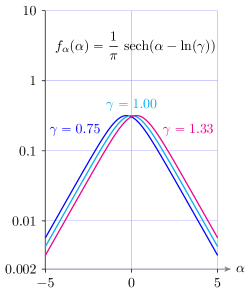
Figure 11: Heavy-tailed example probability distributions. (Left) $f_{\text{a}}\!\left(a\right)$ distribution on a log-log scale. The linear decay of the tail on the log-log plot shows a power law characteristic with decay $a^{-2}$. All moments of the $f_{\text{a}}\!\left(a\right)$ distribution are infinite. (Right) $f_{\alpha}\!\left(\alpha\right)$ distribution on a log-linear scale. All moments of the $f_{\alpha}\!\left(\alpha\right)$ distribution are finite.

Figure 11(right) shows the probability density function of the $f_{\alpha}\!\left(\alpha\right)$ distribution for three choices of $\gamma$. The exponential decay of the PDF is clear from the log-linear plot. All moments of this distribution are finite and the moment generating function (for $\gamma=1$) is,

$$\phi_{\alpha}(\lambda)\>=\>\frac{1}{\cos(\pi\lambda/2)},\quad|\lambda|<1.$$ (28)

The symmetry of (27) about $\alpha=\ln(\gamma)$ shows that,

$$\mu_{\alpha}\>=\>\ln(\gamma).$$

So by applying Theorem 5,

$$\lim_{K\longrightarrow\infty}\operatorname{median}(x_{K})\,=\,0\quad\iff\quad\gamma<1.$$

Note however that for all $\gamma>0$,

$${\cal E}\left[\rule{0.0pt}{8.99994pt}x_{K}\right]\;=\;\infty$$

for all $K$. This is an extreme example of an unstable mean.

The symmetry of the $f_{\alpha}\!\left(\alpha\right)$ distribution implies that the median and mean are equal and the median of the state $x_{K}$ can therefore be given analytically,

$$\operatorname{median}(x_{K}) = \text{e}^{\operatorname{median}(\zeta_{K})}$$

$$= \text{e}^{\operatorname{mean}(\zeta_{K})}\>=\>\text{e}^{K\ln(\gamma)}\>=\>\gamma^{K}.$$

For illustration, and comparison with Figure 7, 500 random trajectories of $\zeta_{K}=\ln(x_{K})$, for $K=1,\dots,100$ are shown in Figure 12. The predicted evolution of the median of $\zeta_{K}$ is compared to a sample-based estimate and found to be accurate. As a result of the very heavy nature of the $f_{\text{a}}\!\left(a\right)$ distribution, the range of the $\zeta_{K}$ trajectories in Figure 12 is much greater than in the normal/lognormal case shown in Figure 7.

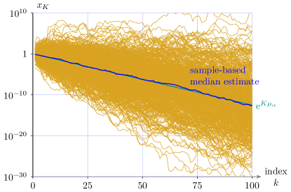
Figure 12: 500 sample trajectory simulations for $\gamma=0.75$. The median of the $\zeta_{K}$ distribution is compared with a sample estimate of the median.

The behaviour of the distribution of $\zeta_{K}$, as $K\longrightarrow\infty$ is given by the distribution of the $K$-fold sum of random variables, $\alpha_{k}$, each drawn from the $f_{\alpha}\!\left(\alpha\right)$ distribution. So the distribution of $\alpha_{K}$ is the $K$-fold convolution of $f_{\alpha}\!\left(\alpha\right)$ and this has been numerically calculated (using the Chebfun Matlab Toolbox [40]) in Figure 13. The characteristics of a sum of hyperbolic secant random variables were first studied in [41].

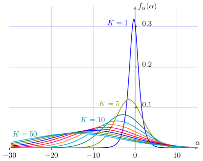
Figure 13: Evolution of the probability distribution function of $\zeta_{K}$ for $K=1,5,\dots,50$. The initial ($K=1$) distribution is that shown in Figure 11(right) for $\gamma=0.75$.

As the moment generating function for $f_{\alpha}\!\left(\alpha\right)$ in (28) is finite in a range around zero the probability that $x_{K}>1$ decays to zero exponentially as $K\longrightarrow\infty$. The bound can be calculated from the moment generating function in (28) and Lemma 10.

$$\operatorname{Prob}\left\{\prod_{k=1}^{K}x_{k}\,>\,1\right\}\;\leq\;\text{e}^{-cK},$$ (29)

where,

$$c\;=\;-\lambda^{*}\ln(\gamma)+\ln\left(\cos(\pi\lambda^{*}/2)\right),$$ (30)

and

$$\lambda^{*}\;=\;\frac{2}{\pi}\arctan\left(\frac{-2\ln(\gamma)}{\pi}\right).$$ (31)

Figure 14 shows this bound. The actual probably can be calculated numerically from the distributions in Figure 13, and estimated from samples in the simulation in Figure 12. Both of these comparisons are made and indicate that the exponent in the Chernoff bound is tight but the bound itself could be divided by a factor of at least two.

Figure 14: Comparison between the Chernoff bound (red) given in (29), (30) and (31) and $\operatorname{Prob}\{x_{K}>1\}$ as a function of $K$ for $\gamma=0.75$. For $K$ up to 50 the numerical evaluation (via Chebfun [40]) of tail of the $K$-fold convolution of $f_{\alpha}\!\left(\alpha\right)$ gives the actual probability and is shown (magenta). For $K>50$ (where numerical limitations prevent the numerical probability calculation) the probability is estimated from 100,000 sample trajectories (blue circles).

This is an extreme example and it is interesting to put it into the context of a simple investment finance problem. Consider the accumulated return on an investment with an independent, identically distributed, random rate of return at every time step. In this context $x_{0}$ is the initial investment, $f_{\text{a}}\!\left(a\right)$ is the probability distribution of the rate of return at each time step, and $x_{K}$ is the investment value after $K$ time steps. Then this example is a case where the expected rate of return is infinite for each of the time steps, and yet the probability of making a profit after $K$ time steps decays exponentially to zero as $K$ increases.

V Discussion

Our goal in this paper has been to precisely specify and illustrate the conditions for the stability of the median, mean and variance in discrete-time stochastic feedback settings. The discrete-time setting enables a far wider range of distributions to be considered than is possible in the continuous-time case, and is at the same time relevant to a wide range of problems. The focus on the scalar variable case is of course much more restrictive and has allowed precise statements to be made about the probability of the distributions of solutions to the difference equations. This is particularly true for the median statistics.

The differences between the stability conditions arise because of the heavy-tailed nature of the resulting distributions. This allows the phenomenon of the mean growing exponentially while the distribution converges exponentially to zero to arise. Note that the stochastic component of the system need not be heavy-tailed for this to be observed; it suffices that the effect of the stochastic component is integrated via a feedback interconnection with a dynamical system.

The variance stability condition given here is a simple case of the more widely known mean-square stability criterion dating from the 1970s [3]. This condition has the advantage that it is also exact for the multi-variable case. However, it is acknowledged that mean-square stability is a strong form of stability [4, p. 136]. This results in this paper emphasise this point, particularly in comparison to median stability.

The conditions for median, mean, and variance stability are different and it is a natural question to consider which is more appropriate for use in any particular problem. Very different answers can arise from the exact statement of the problem and can easily lead to interpretations which are—at least from a cursory point of view—in contradiction. For example, in an investment problem there are a relatively wide range of circumstances in which a return-on-investment will have an expected value greater than one, and consequently the expected profit grows with time, and yet in which the probability of making any profit at all decays to zero. The equivalent conditions in a population dynamics context would indicate that a survival rate may be greater than one and yet the probability of extinction is also going to one.

These apparent paradoxes illustrate that in stochastic feedback situations seemingly similar questions may have widely divergent answers and it is important to pose the correct measure of stability in the problem formulation and the analysis. The increasing use of interconnected feedback networks, and particularly those where online data-based updating leads to stochasticity in the feedback components, requires that we make a careful choice of analysis criteria and design methods.

VI Acknowledgements

The authors would like to thank Tryphon Georgiou, Sean Meyn, Vikram Krishnamurthy, and Subhrakanti Dey for useful discussions on this topic.

References

- [1] R. Kalman, “Control of randomly varying linear dynamical systems,” Proc. Symp. Appl. Math., vol. 13, pp. 287–298, 1962.
- [2] J. C. Willems and G. L. Blankenship, “Frequency domain stability criteria for stochastic systems,” IEEE Trans. Automatic Control, vol. AC-16, no. 4, pp. 292–299, 1971.
- [3] J. Willems, “Mean square stability criteria for stochastic feedback systems,” Int. J. Systems Sci., vol. 4, no. 4545–564, 1973.
- [4] S. Boyd, L. El Ghaoui, E. Feron, and V. Balakrishnan, Linear matrix inequalities in system and control theory. Society for Industrial Mathematics, 1994, vol. 15.
- [5] K. Åström, “On a first-order stochastic differential equation,” International Journal of Control, vol. 1, no. 4, pp. 301–326, 1965.
- [6] G. Blankenship, “Stability of linear differential equations with random coefficients,” IEEE Trans. Automatic Control, vol. AC-22, no. 5, pp. 834–838, October 1977.
- [7] S. Ethier, “The Kelly system maximizes median fortune,” J. Appl. Probability, vol. 41, pp. 1230–1236, 2004.
- [8] H. Kesten, “Random difference equations and renewal theory for products of random matrices,” Acta Math., vol. 131, pp. 207–248, 1973.
- [9] C. M. Goldie, “Implicit renewal theory and tails of solutions of random equations,” Annals of Applied Probability, vol. 1, no. 1, pp. 126–166, 1991.
- [10] A. Brandt, “The stochastic equation with stationary coefficents,” Adv. Appl. Prob., vol. 18, no. 211–220, 1986.
- [11] B. de Saporta, “Tail of the stationary solution of the stochastic equation with Markovian coefficents,” Stochastic Processes and their Applications, vol. 15, pp. 1954–1978, 2005.
- [12] S. Meyn and R. L. Tweedie, Markov Chains and Stochastic Stability, 2nd ed. Cambridge University Press, 2009.
- [13] M. Milisavljević and E. I. Verriest, “Stability and stabilization of discrete systems with multiplicative noise,” in Proc. European Control Conference, 1997, pp. 3503–3508.
- [14] B. Sinopoli, L. Schenato, M. Franceschetti, K. Poolla, M. I. Jordan, and S. S. Sastry, “Kalman filtering with intermittent observations,” IEEE Trans. Automatic Control, vol. 49, no. 9, pp. 1453–1464, 2004.
- [15] N. Elia, “Remote stabilization over fading channels,” Systems & Control Letters, vol. 54, pp. 237–249, 2005.
- [16] ——, “Emergence of power laws in networked control systems,” in Proc. IEEE Conf. on Decision & Control, 2006, pp. 490–495.
- [17] J. Wang and N. Elia, “Distributed averaging under constraints on information exchange: Emergence of Lévy flights,” IEEE Trans. Automatic Control, vol. 57, no. 10, pp. 2435–2449, 2012.
- [18] Y. Mo and B. Sinopoli, “Kalman filtering with intermittent observations: Tail distribtution and critical value,” IEEE Trans. Automatic Control, vol. 57, no. 12, pp. 677–689, 2012.
- [19] S. Dey and L. Schenato, “Heavy-tails in Kalman filtering with packet losses: confidence bounds vs second moment stability,” in Proc. European Control Conference, 2018, pp. 1480–1486.
- [20] A. Rantzer, “Concentration bounds for single parameter adaptive control,” in Proc. American Control Conference, 2018, pp. 1862–1866.
- [21] J. Aitchison and J. Brown, The Lognormal Distribution with special reference to its use in economics. Cambridge University Press, 1957.
- [22] D. Finney, “On the distribution of a variate whose logarithm is normally distributed,” Supplement to J. Royal Statistical Soc., vol. 7, no. 2, pp. 155–161, 1941.
- [23] G. Shellard, “Estimating the product of several random variables,” Journal of American Statistical Assoc., vol. 47, no. 258, pp. 216–221, 1952.
- [24] L. A. Goodman, “The variance of the product of K random variables,” Journal of American Statistical Assoc., vol. 57, no. 297, pp. 54–60, March 1962.
- [25] P. Hall, “On the limiting behaviour of the mode and median of a sum of independent random variables,” Annals of Probability, vol. 8, no. 3, pp. 419–430, 1980.
- [26] S. Bittanti and P. Colaneri, Periodic Systems: Filtering and Control. Springer, 2009.
- [27] J. Roberts and P. Spanos, “Stochastic averaging: an approximate method of solving random vibration problems,” Int. J. Non-Linear Mechanics, vol. 21, no. 2, pp. 111–134, 1986.
- [28] L. Arnold, H. Crauel, and V. Wihstutz, “Stabilization of linear systems by noise,” SIAM J. Control & Optimization, vol. 21, no. 3, pp. 451–461, 1983.
- [29] V. Oseledec, “A multiplicative ergodic theorem; Lyapunov characteristic numbers for dynamical systems,” Trans. Moscow Math. Soc., vol. 19, pp. 197–231, 1968.
- [30] B. Bercu, B. Delyon, and E. Rio, Concentration Inequalities for Sums and Martingales. Springer, 2015.
- [31] F. Cantelli, “Sui confini della probabilità,” Atti del Congresso Internazionale dei Matematici, vol. 6, pp. 47–59, 1928.
- [32] S.-H. Chang, P. C. Cosman, and L. B. Milstein, “Chernoff-type bounds for the Gaussian error function,” IEEE Trans. Communications, vol. 59, no. 11, pp. 2939–2944, 2011.
- [33] R. A. Fischer, “On the ‘probable error’ of a coefficient of a correlation deduced from a small sample,” Metron, vol. 1, pp. 3–32, 1921.
- [34] E. L. Dodd, “The frequency law of a function of variables with given frequency laws,” Annals of Mathematics, vol. 27, no. 1, pp. 12–20, 1925.
- [35] E. Roa, “A number of new generating functions with applications to statistics,” Ph.D. dissertation, Univ. of Michigan, 1924.
- [36] W. Perks, “On some experiments in the graduation of mortality statistics,” J. Institute of Actuaries, vol. 63, no. 1, pp. 12–57, 1932.
- [37] M. J. Fischer, Generalized Hyperbolic Secant Distributions with Applications to Finance. Springer, 2014.
- [38] P. Ding, “Three occurrences of the hyperbolic-secant distribution,” The American Statistian, vol. 68, no. 1, pp. 32–35, 2014.
- [39] W. Harkness and M. Harkness, “Generalized hyperbolic secant distributions,” American Statistical Association Journal, pp. 329–337, March 1968.
- [40] T. Driscoll, N. Hale, and L. Trefethen, Eds., Chebfun Guide. Oxford: Pafnuty Publications, 2014.
- [41] W. Baten, “The probability law for the sum of independent variables, each subject to the law ,” Bull. American Mathematical Society, vol. 40, no. 4, pp. 284–290, 1934.