Morphological Star-Galaxy Separation

Abstract

We discuss the statistical foundations of morphological star-galaxy separation. We show that many of the star-galaxy separation metrics in common use today (e.g. by SDSS or SExtractor) are closely related both to each other, and to the model odds ratio derived in a Bayesian framework by Sebok (1979). While the scaling of these algorithms with the noise properties of the sources varies, these differences do not strongly differentiate their performance. We construct a model of the performance of a star-galaxy separator in a realistic survey to understand the impact of observational signal-to-noise ratio (or equivalently, $5\sigma$ limiting depth) and seeing on classification performance. The model quantitatively demonstrates that, assuming realistic densities and angular sizes of stars and galaxies, 10% worse seeing can be compensated for by approximately 0.4 magnitudes deeper data to achieve the same star-galaxy classification performance. We discuss how to probabilistically combine multiple measurements, either of the same type (e.g., subsequent exposures), or differing types (e.g., multiple bandpasses), or differing methodologies (e.g., morphological and color-based classification). These methods are increasingly important for observations at faint magnitudes, where the rapidly rising number density of small galaxies makes star-galaxy classification a challenging problem. However, because of the significant role that the signal-to-noise ratio plays in resolving small galaxies, surveys with large-aperture telescopes, such as LSST, will continue to see improving star-galaxy separation as they push to these fainter magnitudes.

1 Introduction

Classification of detected objects into stars and galaxies is a basic ingredient for a wide range of science cases for astronomical surveys. At bright magnitudes this problem is relatively simple, since stars outnumber galaxies and the galaxies which do exist are obviously extended on the sky. As surveys push to deeper depths, certainly in the SDSS regime and even more so with surveys on 8-meter class telescopes such as LSST, the statistics become much less favorable for star/galaxy (hereafter abbreviated S/G) separation as galaxy numbers rapidly increase and their apparent size on the sky decreases. This poses a considerable risk for these surveys, particularly for Galactic and stellar science cases where, for example, searches for rare objects or low contrast stellar overdensities in the Galactic halo can be particularly hampered by the “noise” of misclassified galaxies contaminating the stellar sample.

The focus of this work is specifically on morphological separation by distinguishing point-sources from non-point sources (other methods such as color-based separation, e.g. Fadely et al. 2012, are complementary but outside the scope of this work). There are two main steps in the S/G separation problem: the first is to perform some sort of measurement on the pixel values obtained in an image with the goal of constructing a suffient statistic, and the second is to interpret these resulting measurements as a classification into stars or galaxies (either individually or in an ensemble).

The first automated classifiers were developed during the advent of large digitized surveys in the 1970s, owing to the availability of high speed microdensitometers and eventually small CCDs. This necessitated the development of algorithms to summarize this pixel-level data. Sebok (1979) presented one of the first detailed analyses of the S/G separation problem in a Bayesian framework, deriving the theoretically optimal classifier under the assumption of accurate models of the point-spread function (PSF) and galaxies (i.e. an accurate model of the scene). Kron (1980) developed a classifier based on the mean value of inverse squared radius of a source, which would measure deviations from the PSF profile.

A common thread amongst many of these algorithms is the comparison of a pure PSF-fit with a broadened measurement, where the wider profile may or may not have free parameters. Valdes (1982) compared the likelihoods of the observed source over a set of template models, which included both stellar, broadened stellar, and measurement artifact profiles. The SDSS classifier used the ratio of the flux in the best-fit galaxy model to the flux measured with a pure-PSF model. As reported in Lupton et al. (2001), “We initially hoped to use the relative likelihoods of the PSF and galaxy fits to separate stars from galaxies, but found that the stellar likelihoods were tiny for bright stars, where the photon noise in the profiles is small, due to the influence of slight errors in modeling the PSF.” Leauthaud et al. (2007) found that for space-based data, the ratio of the peak surface brightness of an object to the total flux performed better than the neural-network classifier used by Source Extractor (known as CLASS_STAR). More recent versions of Source Extractor have used a parameter spread_model (Desai et al., 2012, and also see Section 2.7 herein), which compares the flux in the PSF fit to the flux in a PSF broadened by a fixed factor (rather than fitting a galaxy model). As we will argue in this work, the commonality of these methods derives from the fact that this type of comparison is closely related to the theoretically optimal Bayesian classification, with the primary differences arising in the handling of noise and deviations from any simplifying assumptions.

After one or more measurements are produced for each source in an image, the task of assigning S/G classifications still remains. Approaches to this problem vary considerably, ranging from the assignment of fixed cut-off values (e.g. SDSS), to decision trees (Weir et al., 1995), neural networks (Odewahn et al., 1992), hybrid ensemble methods (Kim et al., 2015), or Bayesian methods incorporating priors on the object populations (Henrion et al., 2011). In contrast to the similarity of most pixel measurements, the diversity of these methods reflects the fact that there is no single correct way to use a classifier—for a realistic survey the desired trade-off between completeness and contamination, and the evolution of that desired trade-off with signal-to-noise ratio, is a choice that depends on the specific scientific goals of the survey. The tradeoff between completeness and purity of a sample is characterized by the receiver operating characteristic (ROC) curves, which plots these two metrics against each other for a binary classifier.

Our goal in this work is to provide pedagogical but fully technical answers to the following questions:

1. What is the statistical basis for the various pixel-level measurement techniques in common use, and how do they relate to the optimal Bayesian procedure outlined in Sebok (1979)?

2. How can the performance of a classifier on a single object be quantified in terms of the (candidate) galaxy size and the signal-to-noise ratio of the observation? In other words, what is the theoretical information content of a single observation of an object?

3. For a realistic population of objects observed in a survey, what overall performance can be expected under various observing conditions? In particular, can we expect adequate performance in case of LSST, which will survey the sky $\sim 5$ magnitudes deeper than SDSS? Should LSST use the same star-galaxy morphological classification algorithm as SDSS, or could it achieve better performance?

4. How should one combine multiple independent measurements of a star-galaxy separator in a statistically justifiable way? Examples could include repeated measurements of the same type, morphological measurements in different passbands, or combinations of morphological and color-based information.

One topic that we will not address is the treatment of closely-spaced sources, where the light from the sources overlaps on the image and they cannot be treated as isolated from each other. While blended sources are one of the principal challenges of a realistic image processing pipeline, we wish to lay out the theory for isolated sources first without the complication of blending.

In Section 2 we review and compare a number of classification techniques for morphological S/G separation. In Section 3 we evaluate and compare these classifiers with simulated observations using Gaussian light profiles. Section 4 details realistic modeling of the theoretically optimal performance for single objects, using populations of stars and galaxies in a survey such as LSST. We discuss a probabilistic framework for combining multiple independent measurements in Section 5, and summarize our conclusions in Section 6.

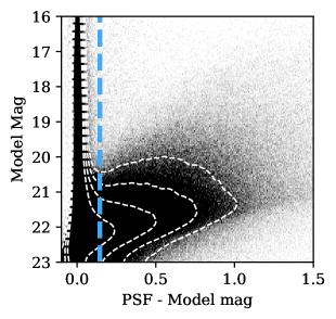
Figure 1: “PSF – Model” classification metric used by SDSS, shown for a set of Stripe 82 observations. The PSF magnitude is the best fitting flux assuming the object is unresolved, while the galaxy model magnitude also fits for an intrinsic size of the object. The stellar locus is at PSF–model = 0, and objects where PSF – model $<0.145$ (dashed vertical line) were classified by SDSS as stars. The plume of galaxies to the right of this division shows good separation at bright magnitudes, but at faint magnitudes tends to merge with the stellar locus due to both the decreasing apparent size of faint galaxies and the less precise measurements of faint objects. Density contours are shown as white dashed lines to illustrate the shape of the distribution.

2 Candidate Classifiers

In this section, we derive and compare expressions for a number of metrics derived from images that can be used for star-galaxy separation. In the following section we compare their performance using analytic Gaussian profiles.

2.1 Morphological Star-Galaxy Separation

Statistically speaking, the problem of morphological star-galaxy separation represents a case of hypothesis testing in frequentist statistics, or a case of model selection in Bayesian statistics (for an introduction and comparison of the two frameworks, see Chapters 4 and 5 in Ivezić et al. 2014, hereafter ICVG). Following the notation from ICVG, we ask whether model $G$ (galaxy) or model $S$ (star) is better supported by data $D$. Here data $D$ are represented by measurements (counts) $\{f_{i}\}$ for $N$ pixels, and their uncertainties, $\sigma_{i}$.

Models $G$ and $S$ give model predictions for data $\{f_{i}\}$. Assuming that the profile corresponding to model $S$ is known (e.g., from analysis of bright stars), and equal to the point-spread-function (PSF), $\phi$,

$$f_{i}^{S}=C_{\textrm{psf}}\,\phi_{i}+{\rm noise},$$ (1)

the only free model parameter is the normalization factor $C_{psf}$, or the so-called “PSF” counts (it is assumed that $\sum_{i=1}^{N}\phi_{i}=1$). To simplify our analysis we are assuming that the position of the source is known a priori and is not a model parameter. In practice, uncertainity in the source center contributes to uncertainty in S/G separation, and covariance between the centroid and the flux measurement may need to be accounted for in the likelihood function for accurate results.

We assume that the galaxy model $G$ is more involved and described by a normalization factor $C_{gal}$ (galaxy model counts) and a vector of additional free model parameters $\theta$,

$$f_{i}^{G}=C_{\textrm{gal}}\,g_{i}(\boldsymbol{\theta})+{\rm noise}.$$ (2)

In the case of the SDSS galaxy models, for example, the vector of free model parameters has three components: axis ratio, position angle, and characteristic radial scale, evaluated for two fixed Sersic indices (exponential profile with $n=1$ and de Vaucouleurs profile with $n=4$) with a parameter $F_{\textrm{deV}}$ controling the fractional contribution of each, and normalized such that $\sum_{i=1}^{N}g_{i}=1$ (again neglecting the centroid.) Our parameterization assumes that the galaxy model function $g(\boldsymbol{\theta})$ “knows” the image PSF, and that the two components can be appropriately convolved together to obtain the model pixel values. In practice, for our modeling we will assume that the PSF and galactic light distribution are both Gaussian, and that the convolved light profile is a Gaussian with width equal to the quadrature sum of the PSF and galaxy widths. This assumption slightly overestimates the accuracy with which galaxies can be measured, since real galaxies are less centrally-concentrated than a Gaussian. In this work we are most interested in the galaxies which are only marginally resolved (and thus are closest to being distinguished by a classifier), so the convolution of the source with the PSF dominates in setting the shape more than the detailed galaxy model. Realistic surveys will of course fit more sophisticated models.

2.2 The Data Likelihood

A common starting point for both Bayesian analysis and the frequentist maximum likelihood and likelihood-ratio analysis, is the likelihood of data. The data likelihood, given a model $M=(S,G)$ and the corresponding model parameters $C$ and $\theta$, as well as prior information $I$, can be expressed as

$$p(D|M,C,\boldsymbol{\theta},I)=\\ (2\pi)^{-N/2}\,\prod\limits_{i=1}^{N}\,\sigma_{i}^{-1}\,\exp\left(-{(f_{i}-f_{i}^{M}(C,\boldsymbol{\theta}))^{2}\over 2\sigma_{i}^{2}}\right),$$ (3)

where we assume that measurements include independent Gaussian noise parametrized by $\sigma_{i}$. Although the data likelihood is often interpreted as “the probability of the data given the model”, it is not properly normalized to be a probability distribution function, PDF (the likelihood of individual data points is a proper PDF).

In frequentist statistics, the maximum likelihood method maximizes $p(D|M,C,\boldsymbol{\theta},I)$ over model parameters $C$ and $\theta$ to obtain their best-fit values, $\hat{C}$ and $\boldsymbol{\hat{\theta}}$ (note that the likelihood itself cannot be interpreted as probabilities for model parameters). The likelihood-ratio test for two models, with likelihoods evaluated with these best-fit parameters, is then used to select the more likely model (when competing models are not nested like here, where the $S$ model is the same as a $G$ model with vanishing intrinsic size, various generalizations of the likelihood-ratio test can be used instead; see Protassov et al. 2002). In other words, an object is declared a galaxy when the maximum likelihood ratio,

$$\Lambda\equiv{p(D|G,\hat{C}_{\textrm{gal}},\boldsymbol{\hat{\theta}},I)\over p(D|S,\hat{C}_{\textrm{psf}},I)}=\\ \prod\limits_{i=1}^{N}\,\exp\left(-{(f_{i}-\hat{C}_{\textrm{gal}}\,g_{i}(\boldsymbol{\hat{\theta}}))^{2}-(f_{i}-\hat{C}_{\textrm{psf}}\,\phi_{i})^{2}\over 2\sigma_{i}^{2}}\right),$$ (4)

is larger than some likelihood-ratio threshold $\Lambda_{SG}$.

The assumption of Gaussianity in the second line of Equation 4 makes $\Lambda$ very brittle, especially in the high signal-to-noise ratio (SNR) limit and in case of non-negligible model errors (i.e. when observed galaxies have profiles different than those included in the model library, or when the point spread function is not adequately modeled).

As discussed earlier, the optimal value of threshold $\Lambda_{SG}$ depends on the desired completeness-purity tradeoff, which implies that it also reflects relative numbers of stars and galaxies in a given sample.

2.3 Maximum likelihood estimate for PSF counts

Before proceeding with a discussion of Bayesian model selection, we briefly review derivation of the maximum likelihood estimate for PSF counts, $C_{\textrm{psf}}$. Using Equations 1 and 3, the data likelihood is

$$p(D|S,C_{\textrm{psf}},I)=\\ (2\pi)^{-N/2}\,\prod\limits_{i=1}^{N}\,\sigma_{i}^{-1}\,\exp\left(-{(f_{i}-C_{\textrm{psf}}\,\phi_{i})^{2}\over 2\sigma_{i}^{2}}\right).$$ (5)

The maximum likelihood value of $C_{\textrm{psf}}$, denoted as $\hat{C}_{\textrm{psf}}$, can be found by maximizing the log-likelihood $\textrm{ln}\,L$:

$$\textrm{ln}\,L(C_{\textrm{psf}})\equiv\ln(p(D|S,C_{\textrm{psf}},I))=\\ {\rm const.}-{1\over 2}\sum_{i=1}^{N}{(f_{i}-C_{\textrm{psf}}\,\phi_{i})^{2}\over\sigma_{i}^{2}},$$ (6)

that is, using the condition $d(\textrm{ln}\,L)/dC_{\textrm{psf}}=0$. The associated uncertainty of $\hat{C}_{\textrm{psf}}$ could be estimated from $\sigma_{C}=(d^{2}(\textrm{ln}\,L)/dC_{\textrm{psf}}^{2})^{-1/2}$, evaluated at $C_{\textrm{psf}}=\hat{C}_{\textrm{psf}}$.

Assuming homoscedastic noise, i.e., $\sigma_{i}\sim\sigma_{0}=$ constant as is the case when the noise is dominated by the background contribution, yields the maximum likelihood estimate

$$\hat{C}_{\textrm{psf}}={\sum_{i=1}^{N}f_{i}\phi_{i}\over\sum_{i=1}^{N}\phi_{i}^{2}},$$ (7)

and its uncertainty (which implies a Gaussian PDF)

$$\sigma_{C}=\sigma_{0}\,\left(\sum_{i=1}^{N}\phi_{i}^{2}\right)^{-1/2}=\sigma_{0}\,(n_{\textrm{eff}}^{\textrm{psf}})^{1/2}.$$ (8)

In the last expression, we have introduced the effective number of pixels, $n_{\textrm{eff}}^{\textrm{psf}}$ (the variance $\sigma_{C}^{2}$ is the sum of variances in each pixel, $\sigma_{0}^{2}$, over the effective number of pixels). For reference, with a Gaussian psf $n_{\textrm{eff}}=4\pi\alpha^{2}$ where $\alpha$ is the Gaussian width in pixels, or $n_{\textrm{eff}}=2.266(\textrm{FWHM})^{2}$ in terms of the Gaussian full-width at half-maximum in pixels (a three-pixel FWHM has $n_{\textrm{eff}}\sim 20$.)

For the case of the broadened model, the maximum likelihood model counts can be estimated as

$$\hat{C}_{\textrm{gal}}={\sum_{i=1}^{N}f_{i}g_{i}(\boldsymbol{\hat{\theta}})\over\sum_{i=1}^{N}g_{i}(\boldsymbol{\hat{\theta}})^{2}},$$ (9)

where the vector of model parameters $\boldsymbol{\hat{\theta}}$ corresponds to the maximum likelihood point.

2.4 The star-galaxy separation based on the likelihood-ratio test

Using Equations 4, 7 and 9, it can be shown that

$$\ln(\Lambda)={1\over 2\sigma_{0}^{2}}\,\left(\hat{C}^{2}_{\textrm{gal}}\sum_{i=1}^{N}g_{i}(\boldsymbol{\hat{\theta}})^{2}-\hat{C}^{2}_{psf}\sum_{i=1}^{N}\phi_{i}^{2}\right),$$ (10)

This expression can be recast as

$$\ln(\Lambda)={1\over 2}\,\textrm{SNR}^{2}\,\left[\left({n_{\textrm{eff}}^{\textrm{psf}}\over n_{\textrm{eff}}^{\textrm{gal}}}\right)\,\left({\hat{C}_{\textrm{gal}}\over\hat{C}_{\textrm{psf}}}\right)^{2}-1\right],$$ (11)

where the PSF signal-to-noise ratio is

$$\textrm{SNR}={\hat{C}_{\textrm{psf}}\over\sigma_{0}\,\sqrt{n_{\textrm{eff}}^{\textrm{psf}}}},$$ (12)

and the effective number of pixels for galaxy profile is

$$n_{\textrm{eff}}^{\textrm{gal}}={1\over\sum_{i=1}^{N}g_{i}(\boldsymbol{\hat{\theta}})^{2}}.$$ (13)

Equation 10 can also be recast as

$$\ln(\Lambda)={1\over 2}\,\left(\chi^{2}_{\textrm{psf}}-\chi^{2}_{\textrm{gal}}\right)\equiv{1\over 2}\,\Delta\chi^{2},$$ (14)

where $\chi^{2}$ is the usual “goodness-of-fit” parameter, evaluated for the maximum likelihood model; therefore, for a galaxy image larger than the PSF size $\Lambda$ increases as the point spread function profile becomes less able to provide a good fit to the observed profile.

2.5 SDSS Classifier

The star-galaxy separator implemented in SDSS image processing pipeline photo (Lupton et al., 2001, 2002) is equal to the difference between the point-spread-function magnitude and the best-fit galaxy model magnitude. This magnitude difference was named concentration by Scranton et al. (2002),

$$c=m_{\textrm{psf}}-m_{\textrm{gal}}.$$ (15)

In the nomenclature of this section, this can also be expressed as

$$c_{\textrm{SDSS}}=2.5\log\left(\frac{\hat{C}_{\textrm{gal}}}{\hat{C}_{\textrm{psf}}}\right).$$ (16)

This expression shows a strong similarity to Equation 11, and indeed these equations can be brought to a close analogy. Since the ratio $(n_{\textrm{eff}}^{\textrm{gal}}/n_{\textrm{eff}}^{\textrm{psf}})$ increases monotonically with the ratio $(\hat{C}_{\textrm{gal}}/\hat{C}_{\textrm{psf}})$, we can write the maximum likelihood estimate as

$$\ln(\Lambda)={1\over 2}\,{\rm SNR}^{2}\,\rho(\hat{C}_{\textrm{gal}}/\hat{C}_{\textrm{psf}})>\ln(\Lambda_{\textrm{SG}}),$$ (17)

where $\rho$ is some monotonic function of the $(\hat{C}_{\textrm{gal}}/\hat{C}_{\textrm{psf}})$ ratio. As a result, a source can be classified as resolved when

$$\left({\hat{C}_{\textrm{gal}}\over\hat{C}_{\textrm{psf}}}\right)>\rho^{-1}\left({2\,\ln(\Lambda_{\textrm{SG}})\over{\rm SNR}^{2}}\right)\equiv\left({C_{\textrm{gal}}\over C_{\textrm{psf}}}\right)_{min}.$$ (18)

Thus for any individual object, the SDSS classifier contains the same information as the likelihood ratio test. However, the likelihood ratio case shows that for a range of observations, the optimal classifier must vary with SNR. SDSS adopted a single value that was optimized for the faint end of their data, which in practice was very effective despite not being theoretically optimal. Because of this, it is likely that some barely-resolved binary stars in SDSS imaging data could be recognized as such by adopting a lower value of $({C_{\textrm{gal}}/C_{\textrm{psf}}})_{\textrm{min}}$ at the bright end.

2.6 Bayesian model selection

To find out which of the two models is better supported by data $D$, in Bayesian framework we compare their posterior probabilities via the model odds ratio in favor of model $G$ over model $S$

$$O_{\textrm{GS}}\equiv{p(G|D,I)\over p(S|D,I)},$$ (19)

where $I$ stands for “prior information”. Note that the concept of “model probability” is distinctively Bayesian. The posterior probability (a number between 0 and 1) of model $M$ ($G$ or $S$) given data $D$, $p(M|D,I)$, follows from the Bayes theorem

$$p(M|D,I)={p(D|M,I)\,p(M|I)\over p(D|I)}.$$ (20)

The marginal likelihood or evidence for model $M$, $p(D|M,I)$, can be obtained using marginalization (integration) over the model parameter space (spanned by $C_{\textrm{gal}}$ and $\theta$ for model $G$, and $C_{\textrm{psf}}$ for model $S$) as

$$E(M)\equiv p(D|M,I)=\\ \int p(D|M,C,\boldsymbol{\theta},I)\,p(C,\boldsymbol{\theta}|M,I)\,dC\,d\boldsymbol{\theta}$$ (21)

The evidence quantifies the probability that the data $D$ would be observed if the model $M$ were the correct model. The evidence is also called the global likelihood for model $M$ because it is a weighted average of the data likelihood $p(D|M,C,\boldsymbol{\theta},I)$, with the priors for model parameters acting as the weighting function.

The hardest term to compute is the probability of the data, $p(D|I)$, but it cancels out when the odds ratio is considered:

$$O_{\textrm{GS}}={E(G)\,p(G|I)\over E(S)\,p(S|I)}=B_{GS}\,{p(G|I)\over p(S|I)}.$$ (22)

The ratio of global likelihoods, $B_{\textrm{GS}}\equiv E(G)/E(S)$, is called the Bayes factor, and is equal to

$$B_{\textrm{GS}}={\int p(D|G,C_{\textrm{gal}},\boldsymbol{\theta},I)\,p(C_{\textrm{gal}},\boldsymbol{\theta}|G,I)\,dC_{\textrm{gal}}\,d\boldsymbol{\theta}\over\int p(D|S,C_{\textrm{psf}},I)\,p(C_{\textrm{psf}}|S,I)\,dC_{\textrm{psf}}}.$$ (23)

The integration of the data likelihood over the model parameter space is an expensive numerical operation. As is well known in Bayesian statistics, and first pointed out in this context by Sebok (1979), the variation of data likelihood around its maximum value can be approximated by a Gaussian (unless the signal-to-noise ratio is very low). In this case, the Bayes factor reduces to the likelihood ratio given by Equation 4, with an additional term accounting for different numbers of free model parameters. The result is related to the Bayesian Information Criterion (BIC, see e.g., Chapter 5 in ICVG) as

$$2\,\ln(B_{\textrm{GS}})\approx\Delta BIC=2\,\ln(\Lambda)-\,M_{\theta}\,\ln(N),$$ (24)

where $M_{\theta}$ is the dimensionality of the vector of free parameters $\theta$, and $N$ is the number of data points. Although the maximum likelihood ratio method is now extended with a “penalty” for increased number of model parameters, this approximation results in identical classification performance as that based on $\Lambda$ alone when the classification cutoff is optimized rather than prescribed a priori.

In the low signal-to-noise ratio limit, integrals from Equation 23 should be explicitly evaluated. Assuming uniform priors for all model parameters,

$$B_{\textrm{GS}}=k\,{\int p(D|G,C_{\textrm{gal}},\boldsymbol{\theta},I)\,dC_{\textrm{gal}}\,d\boldsymbol{\theta}\over\int p(D|S,C_{\textrm{psf}},I)\,dC_{\textrm{psf}}},$$ (25)

where coefficient $k$ depends only on the limits for assumed priors. Here, instead of comparing the maximum values of data likelihoods as in Equation 4, the Bayes factor now compares the mean values of the two data likelihoods over the range of model parameters allowed by priors. Hence, the two classification methods should have different performance, with the maximum likelihood method expected to be inferior. An example of this comparison will be presented in the next section, including a discussion of the Occam’s razor built in the above expression.

2.6.1 Sebok’s ansatz

Sebok (1979) performed a similar analysis to the above in a full Bayesian framework, but added the simplifying assumption that

$$\int p(D|S,C_{\textrm{psf}},I)\,p(C_{\textrm{psf}}|S,I)\,dC_{\textrm{psf}}=p(D|\hat{C}_{\textrm{psf}},I),$$ (26)

and similarly for galaxies. This ansatz allows the integrals from Equation 23 to be replaced with a comparison of the maximum likelihood flux estimates for both models, and results in a likelihood calculation of the same form as Equation 10. Sebok (1979) then required that the term in square brackets in Equation 11 be positive to classify an object as galaxy. This requirement yields a condition

$$\left({\hat{C}_{\textrm{gal}}\over\hat{C}_{\textrm{psf}}}\right)\,\left({n_{\textrm{eff}}^{\textrm{psf}}\over n_{\textrm{eff}}^{\textrm{gal}}}\right)^{1/2}>1.$$ (27)

Compared to Equation 11, Sebok’s ansatz and the assumption of equal priors on star and galaxy density results in the dependence on SNR vanishing.

Sebok (1979) also simplifies the evaluation of this condition by using a single fixed-size galaxy model for comparision, on the basis that it is primarily the marginally-resolved galaxies where the classification is most sensitive and the PSF size dominates in those cases. Despite these differences, we show in the Section 3 that the condition given by Equation 27 acts similarly to the SDSS galaxy separator (in case of Gaussian profiles, Equations 35 and 36 imply a monotonic relationship between the two separators).

2.7 New Star-Galaxy Separator in SExtractor

We also consider a parameter called spread_model, computed by the code SExtractor (Bertin & Arnouts, 1996), that has been recently developed as part of the Dark Energy Survey Data Management program (Mohr et al., 2012). According to Desai et al. (2012), spread_model is a superior star-galaxy classification parameter compared to class_star, SExtractor’s traditional star-galaxy separator (see their Figure 13). The distribution of sources in the spread_model vs. apparent magnitude diagram is reminiscent of the $m_{\textrm{psf}}-m_{\textrm{gal}}$ vs. magnitude diagram constructed with SDSS data (Figure 1).

The spread_model parameter is a normalized simplified linear discriminant between the best-fitting local PSF model ($\Phi$) and a slightly more extended model ($G$) made from the same PSF convolved with a circular exponential disk model with scale length equal to FWHM/16 (here FWHM is the full width at half-maximum of the PSF model). It is defined as (Desai et al., 2012)

$$\texttt{spread\_model}={G^{T}x\over G^{T}\Phi}-{\Phi^{T}x\over\Phi^{T}\Phi}$$ (28)

where $x$ is the image vector centered on the source; see also Soumagnac et al. (2015). The corresponding expression in Desai et al. (2012) has a sign error, which we corrected above (E. Bertin, priv. comm.). For $x=\Phi$, $\texttt{spread\_model}=0$ by construction, and for resolved sources, $\texttt{spread\_model}>0$.

SExtractor also computes spreaderr_model, the uncertainty for spread_model parameter. Using this uncertainty, Bechtol et al. (2015) compute weighted mean of spread_model for a set of images with varying depth, and Koposov et al. (2015) propose a criterion for binary star-galaxy separation that accounts for deteriorating signal-to-noise ratio close to the faint end

$$|\texttt{spread\_model}|<0.003+\texttt{spreaderr\_model}.$$ (29)

Both $G$ and $\Phi$ in Equation 28 are normalized to the observed source flux (in the maximum likelihood sense, c.f. § 2.3). It is easy to show, using nomenclature from this section, that

$$\texttt{spread\_model}=\eta\,\left({\hat{C}_{\textrm{gal}}\over\hat{C}_{\textrm{psf}}}\right)\left({n_{\textrm{eff}}^{\textrm{psf}}\over n_{\textrm{eff}}^{\textrm{gal}}}\right)^{1/2}-1,$$ (30)

where

$$\eta\equiv{(\sum_{i=1}^{N}\phi_{i}^{2})^{1/2}\,(\sum_{i=1}^{N}g_{i}^{2})^{1/2}\over\sum_{i=1}^{N}\phi_{i}g_{i}},$$ (31)

and with an important caveat that the model profile $g$ is fixed, rather than optimized. For a given seeing profile, $\eta$ is fixed and, with the chosen $g$, very close to unity (to within a few percent, see Equation 37 below). Hence, as a comparison with Equations 11 and 27 reveals, spread_model parameter is essentially equivalent to the classifier proposed by Sebok (apart from the fact that here $g$ is fixed).

2.8 Summary of different classifiers

As shown above, there are five closely related candidate classification parameters:

1. SDSS classifer, $C_{\textrm{SDSS}}=2.5\log\left({\hat{C}_{\textrm{gal}}\over\hat{C}_{\textrm{psf}}}\right)$.

2. From Equation 27,
   $C_{\textrm{Sebok}}=\left({\hat{C}_{\textrm{gal}}\over\hat{C}_{\textrm{psf}}}\right)\left({n_{\textrm{eff}}^{\textrm{psf}}\over n_{\textrm{eff}}^{\textrm{gal}}}\right)^{1/2}\\ =10^{(0.4\,C_{\textrm{SDSS}})}\,\left({n_{\textrm{eff}}^{\textrm{psf}}\over n_{\textrm{eff}}^{\textrm{gal}}}\right)^{1/2}$.

3. From Equation 30, $C_{\textrm{spread}}=\eta\,C_{\textrm{Sebok}}-1$.

4. From Equation 11,
   $C_{\Delta\chi^{2}}=\left(\chi^{2}_{\textrm{psf}}-\chi^{2}_{\textrm{gal}}\right)=SNR^{2}\,\left(C_{\textrm{Sebok}}^{2}-1\right)$.

5. From Equation 23, $C_{\textrm{Bayes}}=2\,\ln(B_{\textrm{GS}})$.
   For high SNR, $C_{\textrm{Bayes}}\approx C_{\Delta\chi^{2}}-M_{\theta}\,\ln(N)$.

In addition, when analyzing the behavior of Gaussian profiles in the next section, we will also consider the best-fit profile width, $C_{\sigma}$, as the sixth classification parameter.

Note that the first three classification parameters do not include dependence on the signal-to-noise ratio SNR. In the high SNR limit, all six classifiers are expected to have similar performance. Our aim in the next section is to quantify their behavior in the low SNR limit, using Gaussian profiles. On general statistical grounds, we expect $C_{\textrm{Bayes}}$ to perform the best, and seek to quantify whether its performance gain compared to, e.g., $C_{\textrm{SDSS}}$ or $C_{\Delta\chi^{2}}$, might be significant in practice.

3 Comparison of Classifiers in case of Gaussian profiles

3.1 Outline

In order to compare the statistical properties of the six classifiers summarized in the preceding section, we use an idealized case based on Gaussian profiles for both the source and the PSF. The main goal is to compare their performance in the low-SNR limit. Given SNR, specified by the total number of counts and (Gaussian) noise per pixel, and the values of the PSF width, $\theta_{\textrm{psf}}$, and the intrinsic source width, $\theta_{g}$, we generate a large number of sources (10,000) and equal number of the corresponding PSFs. The profile variations are entirely due to random realizations of the assumed noise. For each source, we fit two free parameters, the profile width and its normalization, using uniform priors (that is, the best fit corresponds to maximum likelihood solution). Given these best-fits, we evaluate the six classification parameters (note that for $C_{\textrm{Bayes}}$ fitting can be bypassed) and compare their distributions for the sources and for the PSFs. Instead of specifying a priori classification threshold, we evaluate the full ROC (receiver operating characteristic) curve, which is a standard tool for quantifying the completeness vs. contamination tradeoff. Although for some classifiers there are some pre-defined numerical values, e.g. a threshold value of 1 for $C_{\textrm{Sebok}}$, or the properties of fixed galaxy profile in case of $C_{spread}$, we optimize over them for a fair comparison of all classifiers. We study the performance of classification parameters as a function of SNR and the $({\theta_{g}/\theta_{\textrm{psf}}})$ ratio. In the rest of this section, we discuss and illustrate these steps in more detail.

3.2 Model profiles and fitting method

We assume a circular Gaussian profile

$$p(r|\alpha)={1\over 2\pi\alpha^{2}}\exp{\left(-{r^{2}\over 2\alpha^{2}}\right)},$$ (32)

which satisfies $2\pi\int_{0}^{\infty}p(r|\alpha)rdr=1$, and $\theta\equiv$ FWHM=2.355$\alpha$. The counts from a source are then described by

$$C(r)=C\,p(r|\alpha)+n(\sigma_{0}),$$ (33)

where $n(\sigma)$ is Gaussian noise with a mean of zero and standard deviation equal to $\sigma$. The source profile width parameter $\alpha$ is a result of the convolution of the PSF and an intrinsic source profile, and is obtained by

$$\alpha=(\alpha_{\textrm{psf}}^{2}+\alpha_{g}^{2})^{1/2}.$$ (34)

We use $\alpha_{\textrm{psf}}$=1.5 pixel, corresponding to $\theta_{\textrm{psf}}=3.5$ pixel (motivated by the median expected seeing for LSST, which has the same $\theta_{\textrm{psf}}$ is pixel units). Given this large $\theta_{\textrm{psf}}$, for simplicity we evaluate the profile at the pixel center. For a Gaussian profile, $n_{\textrm{eff}}=4\pi(\alpha/{\rm pix})^{2}=28.3$.

We get the best-fit values of $C$ and $\alpha_{g}$ by a grid search. Given a 15 pix by 15 pix image generated with chosen input values of $C$, $\alpha_{\textrm{psf}}$, $\alpha_{g}$ and $\sigma_{0}$, we compute the data likelihood $L$ using Equation 3 as a function of two free model parameters, $C$ and $\alpha_{g}$ (and a related quantity $\chi^{2}=-2\ln(L)$). The maximum likelihood best-fit is a pair of ($C$, $\alpha_{g}$) values that maximizes $L$ (or minimizes $\chi^{2}$). An example of such fitting is shown in Figure 2.

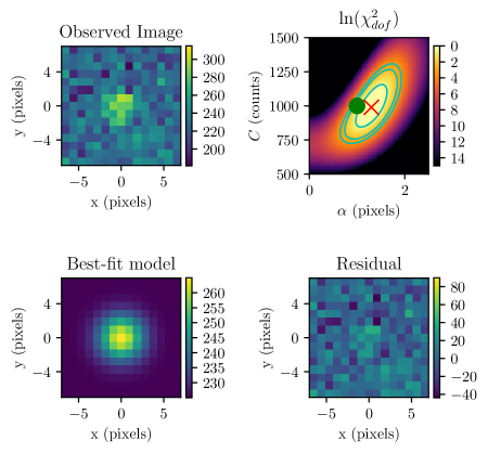
Figure 2: An illustration of fitting an image generated with noise per pixel of $\sigma_{0}=15$ counts, PSF with $\alpha_{\textrm{psf}}=1.5$ pix, the intrinsic profile width $\alpha_{g}=1.0$ pix, and a source with $C=1000$ counts. With an effective number of pixels of $\sim$40, the SNR is $\sim$10. The top left panel shows data image and the top right panel shows the $\chi^{2}$ image as a function of two free parameters, $\alpha_{g}$ and $C$. The standard $1\sigma$, $2\sigma$ and $3\sigma$ contours are shown by the lines, the maximum-likelihood best-fit values of the free parameters by the $\times$ symbol, and the input values of fitted parameters by the dot. The best-fit model is shown in the bottom left panel, and the data-model residuals in the bottom right panel.

3.3 Analytic predictions for Gaussian profiles

Before proceeding with numerical experiments, we summarize analytic predictions for the behavior of classifiers for the case of noise-free Gaussian profiles. For profiles described by $\alpha_{\textrm{psf}}$ (PSF) and $\alpha_{g}$ (source; before convolution with the PSF), it can be shown analytically (and numerically in case of $\eta$) that in the noise-free case,

$$\left({C_{\textrm{gal}}\over C_{\textrm{psf}}}\right)=1+{1\over 2}\,\left({\alpha_{g}\over\alpha_{\textrm{psf}}}\right)^{2},$$ (35)

$$\left({n_{\textrm{eff}}^{\textrm{gal}}\over n_{\textrm{eff}}^{\textrm{psf}}}\right)=1+\left({\alpha_{g}\over\alpha_{\textrm{psf}}}\right)^{2},$$ (36)

and

$$\eta=1+0.06\,\left({\alpha_{g}\over\alpha_{\textrm{psf}}}\right)^{3}.$$ (37)

Hence, all classifiers are only functions of the ratio $(\alpha_{g}/\alpha_{\textrm{psf}})$ and are uniquely related to each other. The differences in the statistical behavior of classifiers are due only to their varying response to noise, as quantitatively discussed below.

The above expressions also elucidate the behavior of classifiers that explicitly depend on SNR. For example, it follows from Equation 11 that ,

$$C_{\Delta\chi^{2}}={\rm SNR}^{2}\,\left({C_{\textrm{gal}}^{2}\,n_{\textrm{eff}}^{\textrm{psf}}\over C_{\textrm{psf}}^{2}\,n_{\textrm{eff}}^{\textrm{gal}}}-1\right)={\rm SNR}^{2}\,\rho\left(\alpha_{g}/\alpha_{\textrm{psf}}\right),$$ (38)

where $\rho(\alpha_{g}/\alpha_{\textrm{psf}})$ is a monotonic function of the ratio $(\alpha_{g}/\alpha_{\textrm{psf}})$ (and note a close relationship to Equation 17). This expression shows that, given a threshold for $C_{\Delta\chi^{2}}$, the smaller values of $\alpha_{g}$ can be “resolved” at a higher SNR. When the star-galaxy separation threshold is optimized at the faint, low-SNR, end of the data, the ability to recognize barely resolved objects at the bright end is not fully exploited. This behavior is generic and not limited to Gaussian profiles as long as $\rho$ is a well-defined monotonic function of $(\alpha_{g}/\alpha_{\textrm{psf}})$.

3.4 Illustration of the $\chi^{2}$ behavior in low SNR case

In the high-SNR regime, the likelihood surface around the maximum likelihood point, such as that shown in the top right panel in Figure 2, can be well approximated by an elliptical Gaussian. As the SNR decreases, the deviations from Gaussianity can be large, with details depending on the profile parameters. Examples of low-SNR likelihood surfaces are shown in Figure 3.

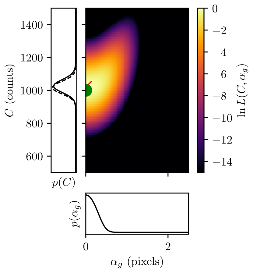
Figure 3: The left panel shows the two-dimensional log-likelihood surface (ln(L)=$-\chi^{2}/2$) for fitting the intrinsic profile width ($\alpha_{g}$) and normalization ($C$, see Equation 33) of an image generated with noise per pixel of $\sigma_{0}=15$ counts, PSF width $\alpha_{\textrm{psf}}=1.5$ pixels, and $\alpha_{g}=1.0$ pixels (same image as shown in the top left panel in Figure 2). The circle marks the true values, and the $\times$ symbol marks the maximum likelihood point. Marginal probability distributions for each parameter are shown to the left and below the panel with solid lines. The dashed line in the panel to the left is the conditional distribution of the normalization $C$ given $\alpha_{g}=0$ (note that its peak corresponds to the maximum likelihood value of PSF counts, $C_{\textrm{psf}}$). The right panel is analogous, except for a profile with $\alpha_{g}=0$ (a noisy realization of the PSF profile). Note that the marginal distributions for $\alpha_{g}$ deviate from a Gaussian shape, especially in the right panel.

3.5 Comparison of Different Classifiers

To compare the behavior of the different classifiers to each other, we created 10,000 random “star” images (with $\alpha_{g}=0$ and $\alpha_{\textrm{psf}}=1.5$) and 10,000 “galaxy” images ($\alpha_{g}=1.0$), all at $\rm{SNR}\approx 10$, which were then classified by all of the algorithms we have considered. Classifier histograms and ROC curves for each classifier’s values are shown in Figure 4, while the different classifiers are plotted against each other in Figure 5. In the ROC panels of Figure 4, the $C_{\textrm{Bayes}}$ curve is shown in each panel by the black dashed line, to provide a visual reference between panels. It is clear from these curves that none of the classifiers do better than the Bayesian result, and with possibly the exception of the $\chi^{2}$ classifier, none of them do substantially worse either. This is despite the rather varied appearance of the classifier histograms; these differences in the values returned for each object do not translate into improved S/G performance, as shown by the ROC curves.

Since we used analytic (Gaussian) profiles, this behavior is easy to understand quantitatively. Expressions listed in §2.8 and §3.3 imply that all classifiers are functions of the $(\alpha_{g}/\alpha_{\textrm{psf}})$ ratio, and thus are uniquely (though non-linearly) related to each other (e.g., $C_{\textrm{SDSS}}$ as a function of the best-fit profile width, see top left panel in Figure 5). The scatter in expected one-to-one relations is seen when at least one of the two plotted classifiers includes explicit SNR dependence (which varies around the input value due to random noise). For example, using expressions listed in §2.8 and §3.3, it is straighforward to show that for Gaussian profiles (see middle left panel in Figure 5)

$$C_{\Delta\chi^{2}}={\rm SNR}^{2}\,{\left(10^{0.4C_{\textrm{SDSS}}}-1\right)^{2}\over 2\,10^{0.4C_{\textrm{SDSS}}}-1}.$$ (39)

The left panel of Figure 6 shows the performance of these classifiers as a function of observation SNR. To do so, it is necessary to distill each ROC curve into a single number; we do so by somewhat arbitrarily reporting the value at which the completeness is equal to the purity. While this is not necessarily the same choice that one would make when performing S/G separation, it is proportional to the overall performance of the classifier (a different choice of a fiducial point will not change the result). While the Bayesian classifier performs somewhat better at very low SNR, at moderate and high SNR the behavior of all classifiers is very similar.

Figure 6 also shows how the Bayesian classifier performs for galaxies of different sizes and at different SNR, but with fixed PSF size. For galaxies similar in size to the PSF (blue dashed line), the performance rapidly improves from relatively modest increases in SNR. Similar gains are also available for objects significantly smaller than the PSF, but only at significantly higher SNR.

We reiterate that Bayesian classifier, although statistically optimal in cases when profile models are known, is brittle in practice and very sensitive to deviations of the observed profiles from assumed models (e.g., galaxies with dust lanes or tidal tails, stars at high SNR).

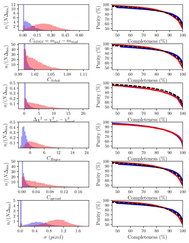
Figure 4: A comparison of the performance of six different classifiers (see §2.8 for definitions) for simulated data. The left column shows distributions of classifier values for 10,000 realizations of a star or galaxy, with noise per pixel of $\sigma_{0}=15$ counts, with blue histograms corresponding to PSF-like sources ($\textrm{SNR}=12.5$) and red histograms to a profile with $\alpha_{g}=1.0$ pix and the same total source counts ($\textrm{SNR}=10.4$.) The right column shows purity vs. completeness ROC curves stars (blue line) and galaxies (red line), where the number of true stars and galaxies in the sample are equal. The dashed black line is the stellar ROC curve for $C_{\textrm{Bayes}}$, replicated to the other plots to aid comparison.

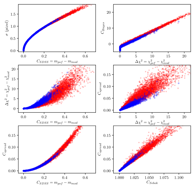
Figure 5: An illustration of correlations between six different classifiers (see §2.8 for definitions). The values for 10,000 random draws are shown, with noise per pixel of $\sigma_{0}=15$ counts, with blue symbols corresponding to PSF-like sources ($\alpha_{\textrm{psf}}=1.5$ pix, $\alpha_{g}=0$) and red symbols to a profile with the same PSF and $\alpha_{g}=1.0$ pix. The distributions of classifier values are shown in Figure 4.

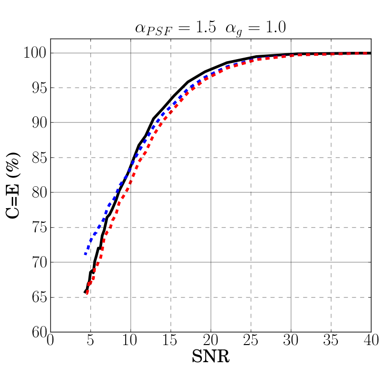
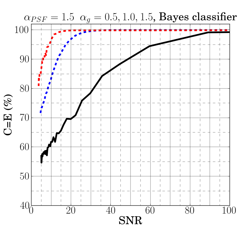
Figure 6: The left panel compares classification performance of different classifiers using the Completeness = Purity point on the ROC curves as metric, for the case $\alpha_{\textrm{psf}}=1.5$ pix and $\alpha_{g}=1.0$ pix. The blue dashed line corresponds to $C_{\textrm{Bayes}}$, the red dashed line to $C_{\Delta\chi^{2}}$ and the other four classifiers are indistinguishable from the black solid line. Note that at SNR=5, $C_{\textrm{Bayes}}$ exceeds the performance of other classifiers by about 7%. The right panel compares the performance of $C_{\textrm{Bayes}}$ for three different values of $\alpha_{g}$ (solid: 0.5 pix; blue dashed: 1.0 pix; red dashed: 1.5 pix).

4 Modeling Star-Galaxy Separation Performance

In this section we show how to predict the star-galaxy separation performance of a particular set of observations, starting only from a pixel-level statistical model of the measurement of individual objects and a simple model of the population of stars and galaxies in the target field. The goal of this modeling is to extract the dependence of star-galaxy separation on the seeing and the signal-to-noise ratio of a given set of observations, and also to show how high SNR observations are able to resolve galaxies with angular size smaller than the size of the PSF.

We first describe how to compute the covariance matrix for objects of a given size and flux using the Fisher matrix formalism. We then combine this result with the true population of stars and galaxies in a given field to obtain a distribution of classifier values as it would be measured in those observations. This is effectively a convolution of the underlying distribution, with the convolution kernel varying across the size-magnitude plane.

4.1 Modeling individual objects

For modeling S/G performance, we need to predict the uncertainty distribution of a chosen star-galaxy separation metric for an object of a given size—which could be zero in the case of a star—and magnitude, under any set of observing conditions. While the Monte Carlo approach from the previous section could be extended to this use case, it is both more illustrative and computationally tractable to approach this analytically using toy models. As we have shown, the various candidate classifiers are in general more similar than they are different, so we will focus on measuring the width of a Gaussian PSF, which may be broadened if the object is a galaxy. We assume that the galaxy light profile is also intrinsically Gaussian. Because the galaxies which are on the verge of being resolved will still have their shape dominated by the PSF, the detailed light distribution in the galaxy is a secondary effect in this context.

We can compute the minimum variance that an unbiased estimator of the observed object size $\hat{\alpha}$ would have via the Fisher information matrix $\mathcal{I}_{\boldsymbol{\theta}}$. This is defined as

$$\mathcal{I}_{\boldsymbol{\theta}}=\mathbb{E}_{I_{1},...,I_{n}\sim f^{n}_{\boldsymbol{\theta}}}\Big{[}\left(\frac{d}{d\boldsymbol{\theta}}\ln L(I_{1},...,I_{n};\boldsymbol{\theta})\right)^{2}\Big{]}$$ (40)

where $I_{n}$ is the measurement of the $n$-th pixel, $\boldsymbol{\theta}$ is a vector of parameters, and $\mathbb{E}$ denotes the expectation value with respect to the function $f_{\boldsymbol{\theta}}$ from which pixel values are drawn.

Our treatment of the Fisher information follows that of Mendez et al. (2013), which showed how to compute the Cramér-Rao bound on astrometric measurements. In this case our interest will be in the accuracy of object size measurements, though the methodology is largely similar. By assuming that the likelihood function can be separated into the product of the likelihoods for each pixel in an object (that is, the noise is not correlated between pixels), one can show that the Fisher information for the measurement of model parameter $\theta$ is

$$\mathcal{I}_{\theta}=\sum_{i=0}^{N}\frac{1}{\sigma_{i}^{2}}\left(\frac{\partial F_{i}(\theta)}{\partial\theta}\right)^{2},$$ (41)

where $F_{i}(\theta)$ denotes the expected value for pixel $i$ of the model being fit to the observations, that is, the noise-free version of Equation 2. The full derivation of this equation is presented in Appendix A. That derivation assumes a Gaussian noise distribution on each pixel, but the result is the same for Poisson noise.

For star-galaxy separation, we will evaluate the Fisher information for the measurement of both the Gaussian width ($\alpha$) and the total flux of the object ($C_{\textrm{gal}}$) under assumed model

$$F_{i}(C_{\textrm{gal}},\alpha)=C_{\textrm{gal}}\,g(r_{i},\alpha)+B,$$ (42)

where $g(r_{i},\alpha)$ denotes the value of a unit-normalized Gaussian of width $\alpha$, evaluated at the radius $r_{i}$ of pixel $i$, the total flux is given by $C_{\textrm{gal}}$, and the background flux $B$.

Evaluating Equation 41 with this model, we obtain

$$\mathcal{I}_{\alpha}=\sum_{i=1}^{N}\sigma^{-2}_{i}\left(C_{\textrm{gal}}\frac{dg(r_{i},\alpha)}{d\alpha}\right)^{2}$$ (43)

$$\mathcal{I}_{\alpha\textrm{Cmod}}=\sum_{i=1}^{N}\sigma^{-2}_{i}g(r_{i},\alpha)\frac{dg(r_{i},\alpha)}{d\alpha}$$ (44)

$$\mathcal{I}_{\textrm{Cmod}}=\sum_{i=1}^{N}\sigma^{-2}_{i}g(r_{i},\alpha)^{2}.$$ (45)

The Fisher matrix containing these elements must then be inverted to obtain the covariance matrix.

In the modeling that follows, we evaluate these functions numerically to compute the S/G performance. To guide our understanding of these results, however, we will also derive a simplified version that characterizes the overall behavior.

Our main quantity of interest is $\mathcal{I}_{\alpha}$, which is inversely proportional to the variance in estimates of the object size. Inserting the Gaussian derivatives into Equation 43 produces

$$\mathcal{I}_{\alpha}=\sum_{i=1}^{N}\frac{C_{\textrm{gal}}^{2}\left(\frac{r_{i}^{2}}{\alpha^{3}}-\frac{2}{\alpha}\right)^{2}g(r_{i},\alpha)^{2}}{C_{\textrm{gal}}\,g(r_{i},\alpha)+B}.$$ (46)

For background-limited observations, we can make the simplifying assumption that individual pixels in the object have values significantly less than the background, such that $C_{\textrm{gal}}\,g(r_{i},\alpha)<B$. This produces

$$\mathcal{I}_{\alpha}=\sum_{i=1}^{N}\left(\frac{r_{i}^{2}}{\alpha^{3}}-\frac{2}{\alpha}\right)^{2}\frac{C_{\textrm{gal}}^{2}\,g(r_{i},\alpha)^{2}}{B}.$$ (47)

This expression can be simplified further by incorporating Equations 12 and 13, and noting that that the $r_{i}^{3}/\alpha^{3}$ term is only significant compared to the $2/\alpha$ term at large radii, but these radii have low weighting in the summation because of the Gaussian function $g(r_{i},\alpha)$. The resulting simplified version is

$$\mathcal{I}_{\alpha}\sim\frac{(\textrm{SNR})^{2}}{\alpha_{\textrm{psf}}^{2}+\alpha_{g}^{2}}.$$ (48)

Seeing and signal-to-noise ratio thus have similar effects on the ability to resolve galaxies. But while seeing has traditionally been understood as the key variable in S/G separation, in practice typical seeing for modern ground-based observatories rarely varies by more than a factor of three to four, even between different sites. The signal-to-noise ratio is far less constrained, and for objects of a given brightness can grow by significant factors either through longer exposure times, larger telescopes, or reduced background. This makes the signal-to-noise ratio the key factor to consider when planning observations or analyzing S/G separation results.

With this qualitative understanding in hand, we can now proceed to a quantitative estimation of S/G performance.

4.2 Modeling Object Populations

We model here distributions of two populations, stars and galaxies, as functions of flux (magnitude) and size.

4.2.1 Galaxy Size and Magnitude Distribution

The general behavior of the underlying distribution of galaxies in the size-magnitude plane is that galaxies become smaller and significantly more numerous at fainter magnitudes. The quantitative description of this distribution is best extracted from space-based data, where there is little confusion between stars and galaxies at the angular sizes that we are concerned with in ground-based observations. For this purpose we use a model that was developed for LSST performance optimization studies, which models the galaxy size distribution as a log-normal function. This was fit to the HST COSMOS-based mock catalogs of Jouvel et al. (2009), which were constructed for optimization of dark energy experiments.

The size distribution as a function of magnitude is well described by a log-normal distribution,

$$p(x=\theta_{\textrm{gal}}|\mu_{\theta},\sigma_{\theta})=(x\sigma_{\theta}\sqrt{2\pi})^{-1}\,\exp\left({-\frac{(\ln x-\mu_{\theta})^{2}}{2\sigma_{\theta}^{2}}}\right),$$ (49)

whose parameters are linear functions of the $i$-band magnitude:

$$\mu_{\theta}=-0.24\,i+5.02\,\,\ln(\textrm{arcsec})$$ (50)

and

$$\sigma_{\theta}=-0.0136\,i+0.778\,\,\ln(\textrm{arcsec}).$$ (51)

The median intrinsic galaxy size (FWHM, in arcsec) is equal to exp($\mu_{\theta}$) and it varies from $\sim 1.0$ arcsec at $i=21$ to 0.35 arcsec at $i=25.3$. An illustration of this model is shown in Figure 7. Figure 8 shows a comparison between these model predictions and the observed COSMOS catalogs from Capak et al. (2007). The observed sizes show a somewhat broader distribution than the log-normal model, but the trends with magnitude are overall sufficiently representative for our modeling.

Figure 7: Model for the distribution of galaxies in the size-magnitude plane, as described in Section 4.2.1. The model assumes a log-normal distribution in size and an exponential distribution over magnitude. The contours are labeled in thousands of stars per square degree per arcsecond FWHM per magnitude.

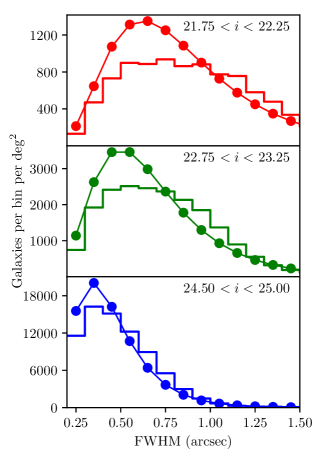
Figure 8: Comparison of the galaxy size distribution from our model (points connected by lines) and the measured object sizes from COSMOS (stepped histogram), in three i-band magnitude bins. While the log-normal model is somewhat more peaked and the real distribution slightly flatter, the overal trend of size and the number counts as a function of magnitude are sufficiently similar for our modeling needs.

For modeling the density of galaxies on the sky, we use a fit to data from the CFHTLS Deep survey (Hoekstra et al., 2006; Gwyn, 2008) from the LSST Science Book (LSST Science Collaboration, 2009). The cumulative galaxy counts between $20.5<i<25.5$ are given by

$$N_{\textrm{gal}}=45\times 10^{0.31(i-25)}\,\,{\rm arcmin}^{-2}.$$ (52)

4.2.2 Stellar Density Distribution

In addition to the model of galaxy counts, our model must also incorporate a stellar density distribution as a function of apparent magnitude. This choice of distribution is subject to much greater variation than the galaxy distribution, as the position of any given survey pointing relative to the Milky Way disk has a very significant impact on the overall normalization and shape of the observed distribution.

Additionally, studies that target stellar samples (and for whom galaxies are the contaminant) are in general not interested in any star, they are nearly always tuned to select stars with specific properties that make them tracers of some target phenomenon. For example, studies of the Milky Way stellar halo often select main sequence turn-off (MSTO) stars via their color because they have roughly constant luminosity and can be used to probe varying distance intervals. The apparent magnitude distribution of MSTO stars thus acts primarily as a proxy for the density distribution as a function of distance and it essentially reflects the structure of the Milky Way. In contrast, the apparent magnitude distribution of a sample of stars without this color-based selection tends to show increasing numbers of red, low-luminosity disk stars at faint magnitudes, even at high Galactic latitudes, and thus also reflects the steepness of the main sequence luminosity function.

In our modeling we will assume that the target stellar sample is the Milky Way halo, rather than nearby stars in the disk. The density profile of the halo can be modeled as a power law which transitions from $r^{-2.5}$ inside of $\sim 25$ kpc (Jurić et al., 2008) to approximately $r^{-3.6}\sim r^{-4}$ in the outer halo (Slater et al., 2016; Cohen et al., 2017). Rather than creating a detailed model for the density distribution along a particular line of sight through the halo, we adopt a constant stellar number density per unit magnitude, which corresponds to an $r^{-3}$ density profile. This is meant to provide a broadly representative approximation of the true halo density profile. As discussed above, the normalization of this profile is strongly dependent on Galactic latitude and longitude, along with color-based selection criteria. We chose to normalize the stellar density such that it equals the density of galaxies at magnitude 20.5, and emphasize that because of the uncertainties in this choice, our focus will be on the variation in S/G separation performance rather than any absolute statements about completeness or purity in a given scenario. Figure 9 shows the ratio of stars to galaxies in our model as a function of magnitude.

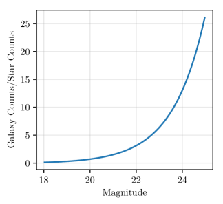
Figure 9: Ratio of the galaxy density to stellar density in the input model. The galaxy and stellar densities are equal at magnitude 20.5.

4.2.3 Convolving the Galaxy Distribution

The left panel of Figure 10, shows examples of the covariance contours from the Fisher matrix modeling that we use as convolution kernels. On a dense grid covering the size-magnitude space, we evaluate for each grid cell the number of galaxies that would be intrinsically present in that cell, then compute the covariance matrix and thus the contribution of that cell to each cell in the as-observed size-magnitude distribution. Summing over these cells produces the distributions shown in the center and right panels of Figure 10. The trend for the “observed” distribution of galaxies to be both wider (due to increased counts and observational scatter) and shifted towards smaller sizes at faint magnitudes can be clearly seen.

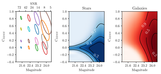
Figure 10: An illustration of the modeling procedure described in Section 4. The left panel shows the covariance ellipses for observations of a grid of galaxies; galaxies at faint magnitudes (or alternatively, low SNR) have large uncertainties in the S/G separation parameter $C_{\textrm{SDSS}}$, while high SNR objects are tightly constrained. The middle panel shows the distribution of measured stellar parameters (magnitude and $C_{\textrm{SDSS}}$) after convolution by the covariance ellipses, while the right panel shows the same model output for galaxies. The contours are labeled with the fraction of objects falling inside each contour. The stars intrinsically lie along $C_{\textrm{SDSS}}=0$, while the galaxies are intrinsically distributed over a wide range of widths (as shown in Figure 7).

4.3 Defining the S/G Separation Criterion

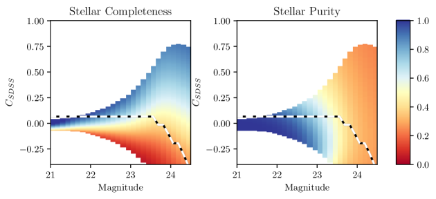
Figure 11: Stellar completeness (left) and purity (right) for an example model ($m_{5}=24.5$ and seeing FWHM of $0.7\arcsec$). At bright magnitudes, the completeness rapidly transitions from 0% to 100% as one moves vertically across the stellar locus at $C_{\textrm{SDSS}}=0$, and the loss of purity (alternatively, increasing contamination) does not begin until very high $C_{\textrm{SDSS}}$ values. At faint magnitudes, the stellar locus is more diffuse and the galaxies begin to dominate in number at small sizes, causing a reduction in stellar purity for separator values close to the stellar locus. Our fiducial separator metric is shown by the dashed black-white line, which traces the point at each magnitude where the completeness is equal to the purity. Areas of very low stellar density are omitted from the colored shading.

The result of this model is a map of the observed sizes and magnitudes of a set of stars and galaxies in a given set of observations. In order to enable quantitative discussion of S/G classification, hereafter we adopt $C_{\textrm{SDSS}}$ classifier. We have yet to apply any sort of classification to the observed set of objects though, and there are many issues that now arise when trying to do so. Defining a morphological classifier is equivalent to drawing some line through the size-magnitude plane that defines two regions (we will focus on a binary classification at the moment and defer discussion of probabilistic classifiers to §5). How one defines this line is entirely dependent on the scientific goals one is trying to achieve. Different levels of contamination and completeness may be acceptable to different science programs and thus a binary classifier that is universally applicable cannot be uniquely defined. We therefore define here a classifier which is sufficiently representative of S/G performance, but is not necessarily what one would always use in practice. We draw a line in size-magnitude space such that, at any given magnitude, the purity of the stellar sample (defined as the number of correctly-labeled true stars divided by all objects classified as stars) is equal to the completeness of the sample of stars (correctly-labeled true stars divided by all true stars).

This separator is illustrated in Figure 11. For a given magnitude column, these plots show what the purity and completeness of a stellar sample would be if everything lower than a chosen y-axis point was classified as a star. This choice of the classifier cutoff can vary with magnitude. As our desired classification goal is for completeness to equal purity, we draw our cutoff (dashed black-white line in Figure 11) such that for every magnitude, the cutoff sits on the same color in both left and right panels of the plot. This is equivalent to a diagonal line in the ROC curve plots. One can see that at faint magnitudes, the classifier must be exceedingly stringent to maintain this criterion, to the extent of reaching 30% completeness or less even by selecting only objects that appear smaller than the PSF (purely for statistical reasons). At some point we decide that such a diminished sample of stars is no longer useful, and we thus define a fiducial completeness level and define the magnitude at which this level is reached as the S/G separation “limit” for this set of observations. This choice is again arbitrary in detail, but will be useful for characterizing the relative S/G performance between different observations. These choices act as means of reducing the dimensionality of the model output, from the completeness and purity planes down to a single number.

4.4 Validating the Model with Stripe 82

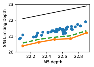
Figure 12: The blue points indiciate measured star/galaxy performance for several Stripe 82 runs (measured at a fiducial point where completeness is equal to purity at 80%) compared to the $5\sigma$ limiting depth of each run. The orange dash-dotted line shows the model prediction for S/G performance over this range of depths (assuming Gaussian PSFs), while the dashed green line accounts for the overestimation of S/G performance due to the imperfect ground-based “truth” catalog. The black line shows where S/G performance equals $5\sigma$ depth, which is unrealistic in practice but shown as a visual aid.

Before any extensive usage of this model, we need to verify that its results accurately characterize the S/G separation performance of real observations. To do so, we need a set of observations under varying seeing and depth conditions, along with a set of “truth” labels for objects in these observations. SDSS Stripe 82 fits these criteria as it consists of numerous repeat observations of the same equatorial stripe, yielding approximately 80 measurements of any given patch of sky, and which were observed in both photometric and various degraded observing conditions (Abazajian et al., 2009). We compare the S/G measurements from these observations those from the Dark Energy Survey, Data Release 1 (Abbott et al., 2018), which is significantly deeper and has better seeing than the SDSS data. In the r-band, the DES data reaches a $\textrm{SNR}=10$ at $24.08$, and has a median seeing of $0.96\arcsec$. This extra depth enables us to use this deep catalog as an approximate “truth” table, since objects which are on the verge of being resolved in the single epoch data, and thus which contribute most to any changes in S/G performance, will be identified in the coadd data. There will still be some unresolved galaxies in this coadded data, and we will discuss the implications and effects of this contamination below.

To model these Stripe 82 performance, we created a stellar density distribution that was normalized to the galaxy density at an r-band magnitude of 20.8, as is seen in the observed Stripe 82 coadd data. The galaxy distribution was the same as measured in COSMOS (see Section 4.2.1). The stellar density model was slightly rising, such that it doubled after two magnitudes of increased depth, again to approximate the observed density distribution.

While our model allows us to specify the observed depth, often characterized by the $5\sigma$ limiting magnitude or “$m_{5}$”, separately from the seeing, in practice these variables are strongly correlated for data from a single telescope even under varying observing conditions. For this reason, we test our model on SDSS assuming that only the $m_{5}$ depth varies independently, and the seeing is linked to this by $m_{5}=\log(0.7/\theta)+C$, where $\theta$ is the seeing FWHM and C is a constant fit to the SDSS data (Ivezić et al., 2019). Reducing the model to one parameter simplifies validation and visualization, but this restriction will be lifted when using the model to make predictions.

For computing the S/G limiting magnitude of the individual Stripe 82 runs, we follow a similar procedure as in the modeling to define the value of $C_{\textrm{SDSS}}$ for each magnitude bin at which the stellar completeness is equal to the purity. This takes advantage of the deeper data in measuring completeness and purity, which most surveys normally lack (otherwise they would simply use the deeper data), but does not introduce the extra uncertainty of trying to estimate these parameters from only the shallow data. This additional information does not improve S/G separation, it only improves our measurement of S/G performance.

Figure 12 shows the result of this verification exercise. The blue points show the depth of individual Stripe 82 runs, while the solid orange line shows the depth estimated using our modeling. In general the reported Stripe 82 S/G depth is somewhat deeper that predicted by the modeling, but some of this difference certainly comes from the ground-based reference catalog used for the comparison, which itself has some contamination fraction. Thus the measured Stripe 82 points slightly overestimate the S/G depth, by failing to recognize some unresolved objects as contaminant galaxies. We roughly estimate the significance of this effect by drawing the dashed line in Figure 12, which mimics this unrecognized contamination by modeling a less-stringent S/G separation purity, equivalent to a 20% unrecognized contamination rate. The resulting model tracks the change of S/G performance with observation depth quite well, although there remains a modest offset of $\sim 0.3$ mag between the absolute predicted performance and the measured performance. As our main interest is in using the model for understanding the seeing and depth dependence of S/G performance, we consider this level of agreement acceptable.

4.5 Model Lessons

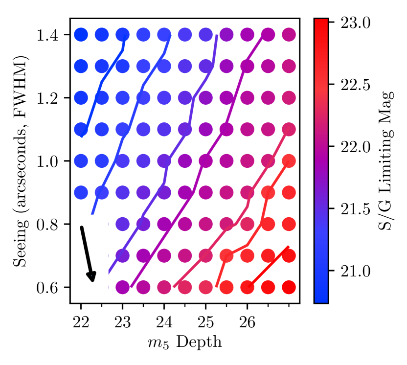
Figure 13: S/G separation limit, defined as completeness equal to purity reaches 80%, as a function of survey seeing and $5\sigma$ limiting depth. The bottom left arrow indicates the vector of changing observational seeing; i.e., the difference between the head and tail represents the $m_{5}$ improvement resulting from a change in seeing alone.

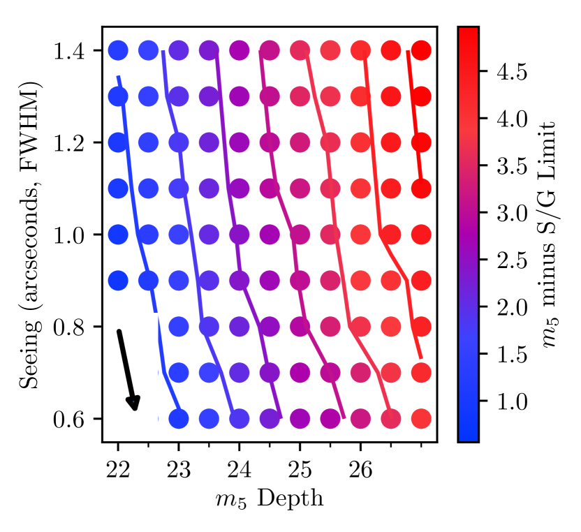
Figure 14: Same as Figure 13, but S/G limiting magnitudes have had the $5\sigma$ depth subtracted. This figure thus shows how the S/G limit diverges from the photometric depth at faint magnitudes.

Figure 15: Left: predicted S/G limiting depth for three example seeing values. These correspond to horizontal slices of Figure 13, and have an average slope of $0.27$ mag S/G per mag $m_{5}$. Right: predicted S/G depth for example $m5$ depths, corresponding to vertical slices of Figure 13. The average slope is $-1.0$ mag S/G per arcsecond of seeing.

For the purpose of discussion in this section, we adopt as the S/G limiting depth the magnitude at which both purity and completeness for stellar sample are 80%. We evaluate it over a grid of $5\sigma$ limiting depths and seeing values, as illustrated in Figures 13 and 14. Several qualitative and quantitative conclusions can be readily derived from features visible in these figures.

These figures show that at constant seeing the S/G limiting depth does not improve as fast as $5\sigma$ limiting depth. For example, in 1 arcsec seeing, the difference $m_{5}-m_{\textrm{SG}}$ increases from about 1.5 mag at $m_{5}=22.5$ to about 2.5 mag at $m_{5}=24.5$. In other words, although $m_{5}$ improved by 2 magnitudes, $m_{\textrm{SG}}$ improved by only 1 magnitude. The same conclusion is valid for other values of seeing (the lines of constant $m_{5}-m_{\textrm{SG}}$ difference in Figure 14 are nearly straight and parallel to each other), and it is a direct result of increasing galaxy-to-star count ratio and decreasing intrinsic galaxy size with magnitude.

When seeing varies, its impact on $m_{5}$ has to be taken into account via $\Delta m_{5}=2.5\log_{10}(\theta_{2}/\theta_{1})$; for example, when seeing improves from 1.4 arcsec (typical for SDSS) to 0.7 arcsec (anticipated as typical for LSST), $m_{5}$ improves by 0.75 magnitudes. In this case, figures show that $m_{5}-m_{\textrm{SG}}$ difference stays approximately constant and thus $m_{\textrm{SG}}$ improves by about 0.75 magnitudes. In order to improve $m_{\textrm{SG}}$ by the same amount in constant seeing, $m_{5}$ would have to be improved by at least 0.75 magnitudes, which implies an increase of exposure time (assuming that background brightness and other observing properties remain unchanged) of at least a factor of 4.

Finally, it is illustrative to compare the performance of star-galaxy separation in our model for fiducial seeing and $m_{5}$ corresponding to SDSS (seeing of 1.4 arcsec and $m_{5}=22.5$) and LSST (seeing of 0.7 arcsec and $m_{5}=27$). While the LSST performance, relative to that of SDSS, will be affected negatively by the increasing galaxy-to-star count ratio and decreasing intrinsic galaxy size with magnitude, it will benefit from better seeing and deeper data. As Figures 13 and 14 show, if LSST had the same seeing as SDSS, due to $m_{5}$ improvement of 4.5 magnitudes, $m_{\textrm{SG}}$ would improve by (only) 1.5 mag (from about 21.0 to 22.5). However, because the seeing is also improved, $m_{\textrm{SG}}$ would improve by about 2.0-2.5 magnitudes (to 23.0-23.5). However, note that this statement is valid only for the definition of $m_{\textrm{SG}}$ adopted here (and it depends strongly on the actual star-to-galaxy count ratio).

5 Probabilistic S/G Separation Cookbook

While the preceding sections have focused on the measurement of images and the expected performance of a classifier, they have not addressed how to best use the results from a catalog of measurements. In this section we present a brief “cookbook” for how a measurement such as $C_{\textrm{SDSS}}$ can be used to construct a probabilistic S/G separator, which will enable the combination of information from multiple measurements in a theoretically sound manner.

The basic outline of the process is as follows:

1. Obtain both survey data and a set of accurate labels. The most common method for obtaining star and galaxy labels is with space-based observations, where galaxies are readily resolved, but other methods such as spectroscopy could also provide this classification. We will assume that these labels are perfectly accurate in our description below. It is also important that data used for training spans the range of SNR and seeing conditions present in the survey for which the classifier will be used, as the probabilistic classification is dependent on the noise properties of the training set matching that of the target observations.

2. Compute $p(c|m,\theta_{\textrm{psf}},\textrm{SNR},[S/G])$. That is, we must construct a function that transforms the raw measurement $c$ from the classifier algorithm (e.g. the SDSS model minus PSF magnitude, and which can have arbitrary scaling) into a properly normalized probability $p(c|\dots)$. One simple way to do this, ignoring for the moment the dependence on magnitude, SNR, and seeing, is to use the high resolution data to separate stars from galaxies, then for each set compute a kernel density estimator on the classifier values measured in the target survey data (one can think of this as a slightly more sophisticated version of histogramming the data as a function of $c$). This function must then be normalized such that the integral over the classifier value $c$, at a given magnitude, is unity. This is $p(c|m,[S/G],\dots)$. Note that this function encodes information about how the measurement of $c$ responds to intrinsic object sizes and shapes in the presence of measurement noise, along with the distribution of object shapes and sizes in the sample. Because of this complexity it is more effective to fit $p(c|m,\dots)$ empirically than to develop a forward model for this function. Additional parameters could be included here to handle effects such as, e.g., PSF chromaticity (Carlsten et al., 2018).

3. Combine multiple measurements of $p(c|S,\dots)$. For objects that are measured multiple times, either in different images or different filters, the appropriate way to combine these measurements is by computing $p(c|S,\dots)$ for each of the different measurements individually and multiply these factors together, i.e.,

   $$L_{S}=\prod_{i=1}^{N}\,p(c_{i}|m,\theta_{\textrm{psf}},{\rm SNR},S),$$ (53)

   and analogously for $L_{G}$. This cannot be done with the classifier value $c$ directly, which is why step 2 in our outline is critical. While it is important that all individual probabilities are properly normalized (the integral over $c$ must be unity), the combined data probability need not be a proper PDF since we will only use it in the ratio of $L_{S}/L_{G}$, where the normalization cancels.

4. Use Bayes’ theorem to obtain $p(G|c,\dots)$ and $p(S|c,\dots)$. Because we require that $p(S|\dots)+P(G|\dots)=1$, we can use Bayes’ theorem to obtain

   $$p(G|\{c_{i}\},m,\theta_{\textrm{psf}},{\rm SNR})=\\ \left[1+\frac{L_{S}\,p(S|m)}{L_{G}\,p(G|m)}\right]^{-1}.$$ (54)

   This equation combines all of the measurements of an object with a prior on the ratio of stars to galaxies. This choice of prior is extremely important, as the ratio of stars to galaxies can vary by more than an order of magnitude across the sky. While one could have empirically used the fitting of the training sample to estimate $p(S)$ or $p(G)$ directly, it would have then carried an assumption that the relative number density of stars and galaxies is the same in the training sample as in the target sample of interest. Computing $p(c|[S/G])$ first decouples these two samples, enabling a training sample at high Galactic latitude, for example, to be used for calibrating S/G separation of a survey at a wide range of stellar densities (though the effects of crowding will at some point alter the properties of the classifier measurement).

The resulting probabilities $p(G|\dots)$ and $p(S|\dots)$ can be directly used in analysis, or as an input to a judiciously chosen classification procedure. For example, if the use case needs a very complete sample of stars, then all objects with $p(S|\dots)>0.5$ could be classified as stars, but if a very clean sample of stars is required, then $p(S|\dots)>0.99$ might be a more appropriate condition. As before, there is no universal optimum and the choice of a position on ROC curve depends on the chosen completeness vs. purity tradeoff. Alternatively, if the desired scientific quantity is the number of stars or galaxies in a region of sky or other parameter-space, simply summing the $p(S)$ or $p(G)$ over all objects in the target region produces an estimate of the number in either class.

As an illustration of probabilistic combination of multiple measurements using eq. 54, we consider a simple case of just two measurements (note that they correspond to likelihoods),

$$p_{G}^{i}\equiv p(c_{i}|m,\theta_{\textrm{psf}},{\rm SNR},G),$$ (55)

with $i=1,2$ and $p_{S}^{i}=1-p_{G}^{i}$. These two measurements could be based on two images in the same bandpass, two images in different bandpasses, or perhaps correspond to one morphological and one color-based measurement. It follows from eq. 54 that the final probability that the source under consideration is resolved is

$$p(G)=\frac{1}{\displaystyle 1+\frac{p(S|m)}{p(G|m)}\frac{(1-p_{G}^{1})(1-p_{G}^{2})}{p_{G}^{1}\,p_{G}^{2}}}.$$ (56)

Note that $p(G)=0$ when at least one of $p_{G}^{1}$ and $p_{G}^{2}$ is zero, and $p(G)=1$ when at least one of $p_{G}^{1}$ and $p_{G}^{2}$ is unity, as intuitively expected. For a given value of the prior $p(S|m)/p(G|m)$, $p(G)$ is a two-dimensional function of $p_{G}^{1}$ and $p_{G}^{2}$, illustrated in Figure 16. The figure shows how high confidence measurements ($>0.9$) can outweigh ambiguous measurements, leading to high confidence of the resulting classification.

Further insight can be obtained by taking the $p_{G}^{1}=p_{G}^{2}$ slice through the top panel of Figure 16. With abbreviations $p_{\textrm{SG}}\equiv p(S|m)/p(G|m)$ and $x\equiv p_{G}^{1}=p_{G}^{2}$,

$$p(G)=\frac{x^{2}}{x^{2}+p_{\textrm{SG}}(1-x)^{2}},$$ (57)

which is illustrated in the lower panel of Figure 16. As evident, $p(G)$ is a monotonic function of $x$, with a value of $x$ that corresponds to $p(G)=0.5$ strongly dependent on the prior $p_{\textrm{SG}}$. Consider two uninformative measurements, $x=0.5$. When $p_{\textrm{SG}}=1$, the final probability remains uninformative, $p(G)=0.5$. However, when $p_{\textrm{SG}}=10$, for example, this prior that strongly favors $S$ results in $p(G)=0.09$ (and symmetrically, $p(G)=0.91$ for $p_{\textrm{SG}}=0.1$). On the other hand, when measurements strongly favor $G$, e.g. $x=0.9$, then $p(G)=0.99$ for $p_{\textrm{SG}}=1$ and $p(G)=0.89$ even when $p_{\textrm{SG}}=10$ (and $p(G)=0.999$ for $p_{\textrm{SG}}=0.1$). Overall, ambiguous measurements lean towards the prior, while high confidence measurements are required when the underlying prior strongly disfavors a particular classification. As always, an evaulation of the ROC curve is still required to deliver the desired completeness and contamination properties for a given scientific use case.

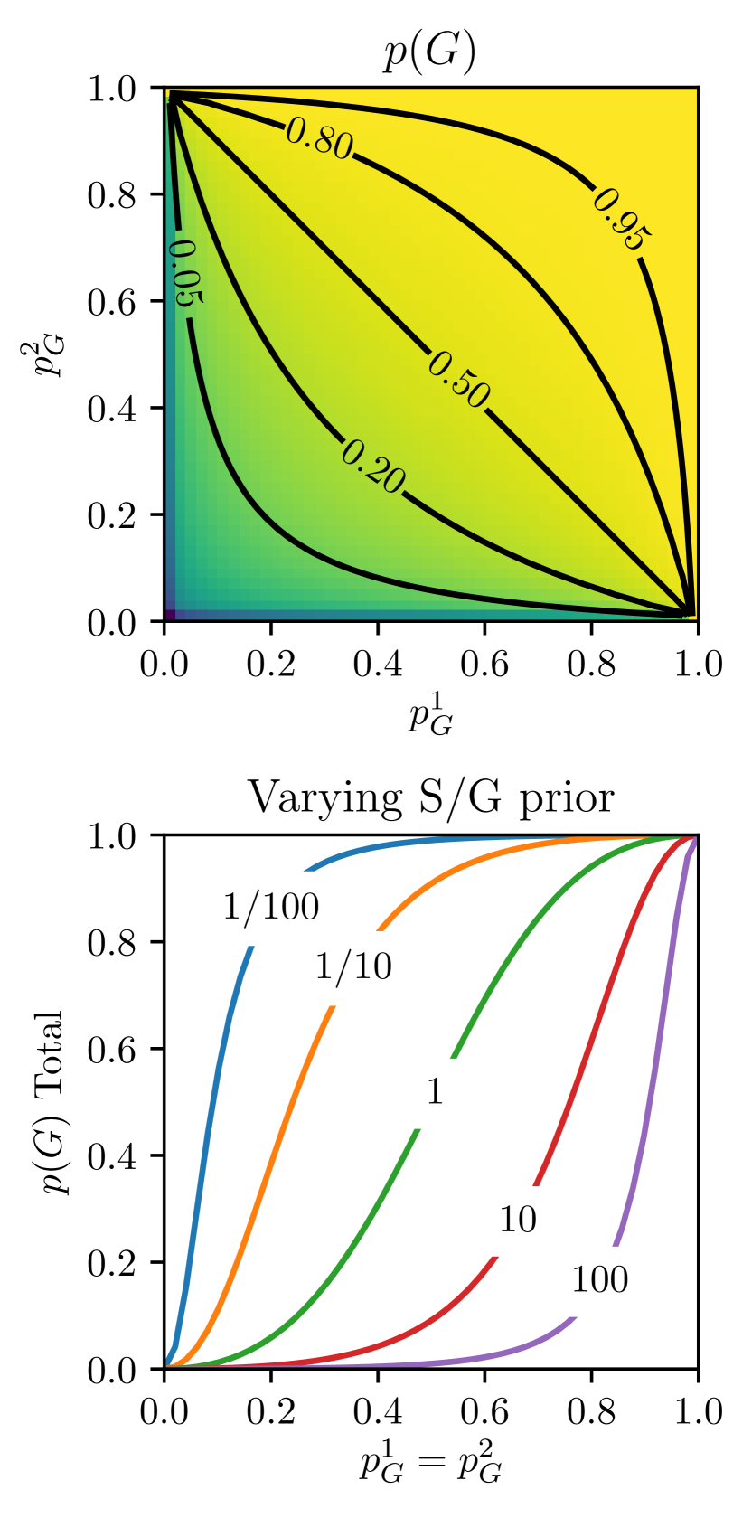
Figure 16: Top: Combined probabilitiy of that an observed object is a galaxy, given two input measurements $p_{G}^{1}$ and $p_{G}^{2}$, and assuming an equal density of stars and galaxies as a prior. Bottom: Combined probability, given two input measurements which are equal to each other, but under varying assumed priors for the ratio of stars to galaxies. These correspond to slices along the lower-left to upper-right diagonal of the top panel.

6 Discussion and Conclusion

Our work has also shown that many of the commonly used measurement techniques for S/G separation are all closely related to each other, and also related to the theoretically optimal technique described by Sebok (1979). The resulting performance of these classifiers is thus very similar, with the primary differences resulting from their treatment of noise and the evolution of their numerical values with SNR or depth. These similarities suggest that the measurements on the pixels themselves are unlikely to see dramatic improvement from new algorithms. There are of course simplifying assumptions in our analysis that may be addressed by practical implementations of these techniques, and gains in S/G performance to be had from such methods, but the basic comparison of a broadened profile with a PSF profile appears firmly planted.

Our modeling of the theoretical performance of an idealized S/G classifier emphasizes the importance of the image SNR on the resulting completeness and contamination. This is often under-appreciated, and angular resolution is often assumed to be the key factor in S/G performance. The distinction between these two mechanisms is subtle but significant. Low SNR objects have poorly-constrained size measurements, making it difficult to distinguish PSF-shaped objects from broadened ones. Deeper observations can increase the SNR of objects, which enables more precise shape measurement and thus better S/G separation. Such deeper observations can come from longer exposure times, better seeing, or by observing on a larger-aperture telescope.

Improved seeing also increases the observed size difference between point sources and galaxies of a given size, and hence enables less precise (lower SNR) size measurements to successfully distinguish stars from galaxies. This effect is obviously well-known, but we emphasize in this work that a substantial portion of its apparent effectiveness is due to the improved SNR in better seeing conditions.

To fully take advantage of the information in high SNR images, however, the image PSF must be precisely characterized. It is beyond the scope of this work to quantify the effect of errors in the PSF model, but it is clear that systematic errors in S/G separation can be introduced by the use of a poor quality PSF model. Extra caution must be used when trying to classify small objects (relative to the PSF size) using high SNR data, since spatial or chromatic PSF variations or detector effects may be relatively more significant, rather than obscured in the noise.

Surveys on 8-m class telescopes, such as the Hyper Suprime-cam Survey and LSST, will place strong demands on S/G separation, relying on SNR to overcome the increasing numbers of galaxies at faint magnitudes. Extracting the most stellar and Galactic science from these surveys will require careful attention at all stages of survey design, image processing, and statistical treatment of the resulting catalogs.

Additionally, the challenge of deep S/G separation on 8-meter class surveys will increase the importance of combining all available information when classifying objects, across images, passbands, and including non-morphological information such as colors or proper motion measurements. We have outlined a blueprint of a procedure for this. Converting each individual type of measurement to a probabilistic form also enables the user to apply appropriate priors, such as models of the star and galaxy density distributions or measurements from other surveys. Placing S/G separation on a rigorously probabilistic basis will maximize the scientific return of these surveys.

Appendix A Fisher Information calculation

In this appendix we derive the Fisher information for a set of pixels $f_{n}$ which are drawn from a Gaussian distribution, and where the expected mean values are

$$f_{n}=C_{\textrm{gal}}g_{i}(\theta)+B,$$ (A1)

where $g_{i}(\theta)$ is the galaxy model with a vector of shape parameters $\theta$, B is a constant background level across all pixels, and $C_{\textrm{gal}}$ is the total flux of the object.

The Fisher information is defined as

$$\mathcal{I}_{\theta}=\mathbb{E}_{f_{1},...,f_{n}\sim f_{\theta}^{M}}\left[\left(\frac{\partial}{\partial\theta}\ln L(f_{1},...,f_{n};\theta)\right)^{2}\right]$$ (A2)

where $f_{n}$ is the measured value of pixel $n$. Our likelihood function $L(f_{1},...,f_{n};\theta)$ was defined earlier in Equation 3 as $p(D|M,C,\theta)$. Inserting this likelihood function and dropping terms inside the partial derivative with no dependence on $\theta$ yields

$$\mathcal{I}_{\theta}=\mathbb{E}_{f_{1},...,f_{n}\sim f_{\theta}^{M}}\left[\left(\frac{\partial}{\partial\theta}\sum_{i=0}^{N}\frac{-[f_{i}-F_{i}(\theta)]^{2}}{2\sigma_{i}^{2}}\right)^{2}\right],$$ (A3)

where $F_{i}(\theta)$ denotes the expected value for pixel $i$ of the model being fit to the observations (i.e., the noise-free version of Equation 2.)

Evaluating the derivative,

$$\mathcal{I}_{\theta}=\mathbb{E}_{f_{1},...,f_{n}\sim f_{\theta}^{M}}\left[\left(\sum_{i=0}^{N}-\frac{\partial F_{i}(\theta)}{\partial\theta}\frac{\left[f_{i}-F_{i}(\theta)\right]}{\sigma_{i}^{2}}\right)^{2}\right].$$ (A4)

We then assume that the measurement residuals are uncorrelated, that is,

$$\mathbb{E}_{f_{1},...,f_{n}\sim f_{\theta}^{M}}\left[\left[f_{i}-F_{i}(\theta)\right]\left[f_{j}-F_{j}(\theta)\right]\right]=0$$ (A5)

for all $(i,j)$ where $i\neq j$. This enables us to obtain

$$\mathcal{I}_{\theta}=\mathbb{E}_{f_{1},...,f_{n}\sim f_{\theta}^{M}}\left[\sum_{i=0}^{N}\left(\frac{1}{\sigma_{i}^{2}}\frac{\partial F_{i}(\theta)}{\partial\theta}\right)^{2}\left[f_{i}-F_{i}(\theta)\right]^{2}\right].$$ (A6)

Pulling the summation out of the expectation value, and using the fact that

$$\mathbb{E}_{f_{i}\sim f_{\theta}^{M}}\left[(f_{i}-F_{i}(\theta))^{2}\right]=\sigma_{i}^{2}$$ (A7)

we obtain

$$\mathcal{I}_{\theta}=\sum_{i=0}^{N}\frac{1}{\sigma_{i}^{2}}\left(\frac{\partial F_{i}(\theta)}{\partial\theta}\right)^{2}.$$ (A8)

This is directly analogous to the solution in the case of Poisson noise (from Mendez et al. 2013), which is

$$\mathcal{I}_{\theta}=\sum^{N}_{i=1}\frac{1}{\lambda_{i}(\theta)}\left(\frac{d\lambda_{i}(\theta)}{d\theta}\right)^{2}$$ (A9)

where $\lambda_{i}$ is the expected value in pixel $i$.

References

- Abazajian et al. (2009) Abazajian, K. N., Adelman-McCarthy, J. K., Agüeros, M. A., et al. 2009, ApJS, 182, 543
- Abbott et al. (2018) Abbott, T. M. C., Abdalla, F. B., Allam, S., et al. 2018, ApJS, 239, 18
- Bechtol et al. (2015) Bechtol, K., Drlica-Wagner, A., Balbinot, E., et al. 2015, ApJ, 807, 50
- Bertin & Arnouts (1996) Bertin, E., & Arnouts, S. 1996, A&AS, 117, 393
- Capak et al. (2007) Capak, P., Aussel, H., Ajiki, M., et al. 2007, ApJS, 172, 99
- Carlsten et al. (2018) Carlsten, S. G., Strauss, M. A., Lupton, R. H., Meyers, J. E., & Miyazaki, S. 2018, MNRAS, 479, 1491
- Cohen et al. (2017) Cohen, J. G., Sesar, B., Bahnolzer, S., et al. 2017, ApJ, 849, 150
- Desai et al. (2012) Desai, S., Armstrong, R., Mohr, J. J., et al. 2012, ApJ, 757, 83
- Fadely et al. (2012) Fadely, R., Hogg, D. W., & Willman, B. 2012, ApJ, 760, 15
- Gwyn (2008) Gwyn, S. D. J. 2008, PASP, 120, 212
- Henrion et al. (2011) Henrion, M., Mortlock, D. J., Hand, D. J., & Gandy, A. 2011, MNRAS, 412, 2286
- Hoekstra et al. (2006) Hoekstra, H., Mellier, Y., van Waerbeke, L., et al. 2006, ApJ, 647, 116
- Ivezić et al. (2014) Ivezić, Ž., Connolly, A., Vanderplas, J., & Gray, A. 2014, Statistics, Data Mining and Machine Learning in Astronomy (Princeton University Press)
- Ivezić et al. (2019) Ivezić, Ž., Kahn, S. M., Tyson, J. A., et al. 2019, ApJ, 873, 111
- Jouvel et al. (2009) Jouvel, S., Kneib, J. P., Ilbert, O., et al. 2009, A&A, 504, 359
- Jurić et al. (2008) Jurić, M., Ivezić, Ž., Brooks, A., et al. 2008, ApJ, 673, 864
- Kim et al. (2015) Kim, E. J., Brunner, R. J., & Carrasco Kind, M. 2015, MNRAS, 453, 507
- Koposov et al. (2015) Koposov, S. E., Belokurov, V., Torrealba, G., & Evans, N. W. 2015, ApJ, 805, 130
- Kron (1980) Kron, R. G. 1980, ApJS, 43, 305
- Leauthaud et al. (2007) Leauthaud, A., Massey, R., Kneib, J.-P., et al. 2007, ApJS, 172, 219
- LSST Science Collaboration (2009) LSST Science Collaboration. 2009, ArXiv e-prints, arXiv:0912.0201
- Lupton et al. (2001) Lupton, R., Gunn, J. E., Ivezić, Z., Knapp, G. R., & Kent, S. 2001, in Astronomical Society of the Pacific Conference Series, Vol. 238, Astronomical Data Analysis Software and Systems X, ed. F. R. Harnden, Jr., F. A. Primini, & H. E. Payne, 269
- Lupton et al. (2002) Lupton, R. H., Ivezic, Z., Gunn, J. E., et al. 2002, in Society of Photo-Optical Instrumentation Engineers (SPIE) Conference Series, Vol. 4836, Survey and Other Telescope Technologies and Discoveries, ed. J. A. Tyson & S. Wolff, 350–356
- Mendez et al. (2013) Mendez, R. A., Silva, J. F., & Lobos, R. 2013, PASP, 125, 580
- Mohr et al. (2012) Mohr, J. J., Armstrong, R., Bertin, E., et al. 2012, in Proc. SPIE 8451, Software and Cyberinfrastructure for Astronomy II, Vol. 8451
- Odewahn et al. (1992) Odewahn, S. C., Stockwell, E. B., Pennington, R. L., Humphreys, R. M., & Zumach, W. A. 1992, AJ, 103, 318
- Protassov et al. (2002) Protassov, R., van Dyk, D. A., Connors, A., Kashyap, V. L., & Siemiginowska, A. 2002, ApJ, 571, 545
- Scranton et al. (2002) Scranton, R., Johnston, D., Dodelson, S., et al. 2002, ApJ, 579, 48
- Sebok (1979) Sebok, W. L. 1979, AJ, 84, 1526
- Slater et al. (2016) Slater, C. T., Nidever, D. L., Munn, J. A., Bell, E. F., & Majewski, S. R. 2016, ApJ, 832, 206
- Soumagnac et al. (2015) Soumagnac, M. T., Abdalla, F. B., Lahav, O., et al. 2015, MNRAS, 450, 666
- Valdes (1982) Valdes, F. 1982, in Proc. SPIE, Vol. 331, Instrumentation in Astronomy IV, 465–472
- Weir et al. (1995) Weir, N., Fayyad, U. M., & Djorgovski, S. 1995, AJ, 109, 2401