Lightweight and Robust Representation of Economic Scales
from Satellite Imagery

Abstract

Satellite imagery has long been an attractive data source providing a wealth of information regarding human-inhabited areas. While high-resolution satellite images are rapidly becoming available, limited studies have focused on how to extract meaningful information regarding human habitation patterns and economic scales from such data. We present READ, a new approach for obtaining essential spatial representation for any given district from high-resolution satellite imagery based on deep neural networks. Our method combines transfer learning and embedded statistics to efficiently learn the critical spatial characteristics of arbitrary size areas and represent such characteristics in a fixed-length vector with minimal information loss. Even with a small set of labels, READ can distinguish subtle differences between rural and urban areas and infer the degree of urbanization. An extensive evaluation demonstrates that the model outperforms state-of-the-art models in predicting economic scales, such as the population density in South Korea ($R^{2}$=0.9617), and shows a high use potential in developing countries where district-level economic scales are unknown.

Introduction

Satellite images captured through remote sensing technology provide useful information regarding human activities and land covers without having to visit the region. Analyzing satellite images provides new insights for establishing policies and for understanding population-level behaviors in districts and broader areas. Another advantage of satellite imagery is its ability to search historical data, which can reveal the temporal dynamics of specific locations. Several techniques have been proposed to analyze satellite images.

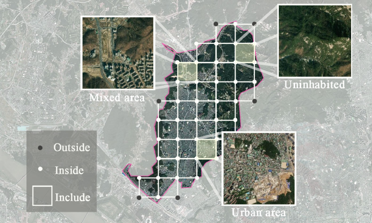
Figure 1: Methods for selecting satellite imagery of target districts. Unlike the previous methods (?), our neural network model can utilize all image tiles belonging to the target. At least three points should belong to the district. The mixed area is a mixed landscape composed of urban and rural interaction.

Many studies measure the critical factors of socioeconomic scales from satellite images, and the demand has been rapidly increasing. For example, demographic research represents a popular application area in which scholars have leveraged the light intensity of nighttime satellite images to extract economic activities (?; ?; ?). Nighttime satellite images have also been used to predict the population density of counties in the United States (?). Although nighttime images are subject to noise, such as saturation effects, they have shown to yield a meaningful linear relationship between brightness and various economic scales.

More recently, high-resolution daytime satellite imagery has emerged as an attractive data source that could reveal fine-grained information at an unprecedented scale. For example, transfer learning has been used to extract socioeconomic indicators to create an accurate poverty map of Uganda (?). Such research has considerable implications for sustainable development growth in developing countries. A convolutional neural network (CNN) has been used to predict grid cell estimates of county-level population counts (?). This work produced a high-resolution grid-shaped population map from satellite images at a 30 arc-second resolution ($\approx$ 1$km^{2}$). However, this method is not applicable outside of the United States because conventional statistics are produced based on districts that can be of any polygon shape rather than at the grid-level, which leads to a mismatch when attempting to use satellite images.

The method proposed in this paper is inspired by the mean-teacher model in semi-supervised learning (?) and the full-convolution CNN model with transfer learning capacity used to predict poverty (?). Our method, which is called ‘Representation Extraction over an Arbitrary District’ (READ), utilizes daytime satellite image tiles whose three vertices belong entirely to the polygon representing each district. This method is depicted in Fig. 1. As the picture demonstrates, a single district can contain vastly different land covers such as urban built-up, water, forest, etc. Our task is to learn these sophisticated spatial features of an arbitrarily shaped district based on high-resolution satellite images to produce a fixed-length representation of economic scales.

The model has considerable implications for monitoring the urbanization process not only in developing countries but also in developed countries. Cities are rapidly evolving; however, it is far slower to detect this process, often using decade-cycled demographic surveys. Notably, these surveys are even extraordinarily costly and time-consuming; our model offers a possible alternative with a reasonable budget and time requirement. Our method can measure diverse urban phenomena such as urban sprawl with improved temporal resolution.

READ is a lightweight method of measuring economic scales from high-resolution images. The learned features are robust to the size of the original labels. They are highly informative when estimating critical economic scales, such as population density, age, education, income, etc. We present a comprehensive evaluation of the model based on a rich set of data from one developed country, South Korea, and demonstrate its potential use in a developing country, Vietnam. The code is released at GitHub.

Related works

Satellite images have become available for public use. These images allow the constant monitoring of the earth and reveal the detailed land cover during both nighttime and daytime, rendering them an excellent resource for the prediction of human activities. Nighttime satellite images are in a lower resolution and have been used to predict the gross domestic product (?; ?), energy consumption (?; ?), epidemic fluctuations (?), and regional economic productivity (?) at the national level. In contrast, high-resolution daytime satellite imagery can reveal detailed land appearance over smaller areas.

Scholars have applied daytime satellite images to a CNN-based model of the Visual Geometry Group 16 (VGG16) architecture to predict the population density (?). Other scholars (?) used 250m-resolution Landsat-7 satellite imagery as input to estimate the population density of Kenya. A regression model was used in the study, while a subsequent study (?) used a classification model to determine the electricity use levels of the population using US Census Summary Grids. Furthermore, This approach (?) is used to integrate nighttime lighting data with 30m-resolution Landsat-8 satellite images and apply machine learning techniques to detect urban markets that help capture real economic activity. The latest study conducted by Facebook Research and Columbia University released an online high-resolution population density map of Africa and Asia (?). Their basic idea is to perform a binary classification of each satellite image that verifies the existence of a building and rankings the likelihood of an area having urban structures. While previous models had adapted VGG for training, this new model applied residual neural nets. This work contributed to the construction of the gridded population of the world version 4 (?), which is known as the current state-of-the-art global population density map.

Satellite images have also been used for poverty prediction. At the national level, a previous study reported a linear relationship between nighttime lights and the percent of the population living on $2 per day or less using the Defense Meteorological Satellite Program (DMSP) F-15 images (?). Another study predicted the income level in India using developmental statistics (?). These authors trained a convolutional network to predict parameters and income levels. However, the parameters utilized in this model are specific to the country analyzed.

Deep learning methods can predict demographic information through satellite images at the national level. The performance of models trained using supervised learning largely depends on the quality and number of the labeled data (?). This is because of the lack of labeled data, which makes it challenging to train deep neural networks. A recent study proposed a novel approach to address this deficiency by adopting two-staged transfer learning and testing a linear regression of fine-tuned feature extractors (?). However, this method is subject to noise because the satellite images had to be randomly chosen for each target area to reduce the computation overhead. Compared to this study, the current paper proposes to utilize all available images instead of sampling via its unique lightweight structure. Our approach also enables computation over smaller and flexible geographical boundaries.

Model

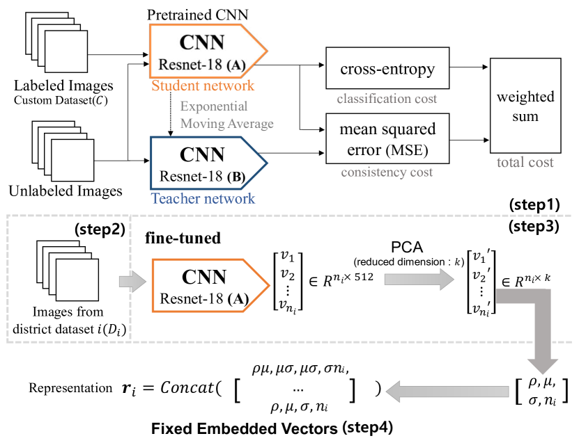
Figure 2: Our model operates in four steps: (step1) training embedding via semi-supervised learning and transfer learning, (step2) data pruning, (step3) dimensionality reduction, and (step4) calculating the embedded spatial statistics and conducting regression for validation.

We first state the problem. Let $d_{j}^{i}$ be the $j$-th satellite imagery of district $i\in U$, where $U$ is the complete set of districts in a country. Let $D_{i}$ be the set of satellite imagery of district $i$. Since districts can be of any shape and size, the number of satellite images in $D_{i}$ varies from one district to another. We define this number for district $i$ as $n_{i}$, i.e., $d_{j}^{i}\in D_{i}$ where $1\leq j\leq n_{i}$. Then, the main problem is defined as follows:

Problem:  Given an image set $D_{i}$ of district $i$, can we extract fixed-sized ($s$) representations $\mathbf{r}_{i}$ (i.e., $\mathbf{r}_{i}\in\mathbf{R}^{s}$ of any district $i$) and predict $y_{i}$ the attribute of interest in the district $i$?

In Fig. 1, this would be equivalent to extracting a representation and predicting the related attributes of a district given its complete set of satellite image tiles.

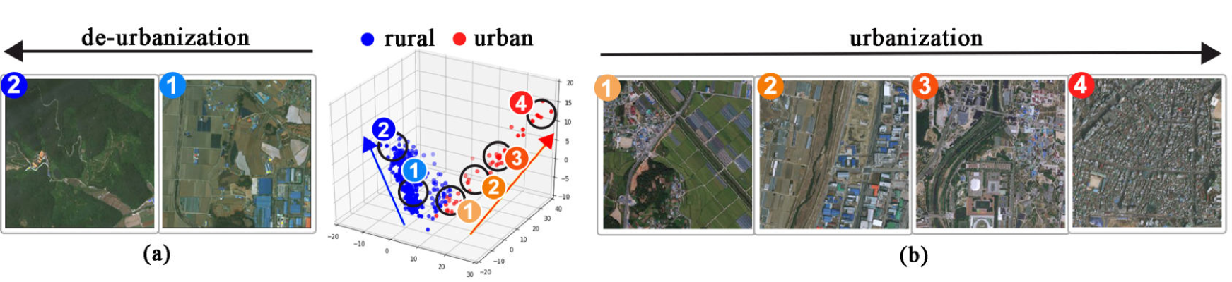
Figure 3: Embedded space analysis shows that rural images (blue) are well separated from more urban images (red). For the blue cluster, as we observe images from anchor points 1 to 2, the de-urbanization trend becomes more pronounced. In contrast, for the red cluster, as we observe images from anchor points 1 to 4, the degree of urbanization becomes more intense.

Training embedding via semi-supervised learning and transfer learning

Network learning with supervision was used to extract meaningful information from satellite imagery. We constructed a labeled custom dataset ($\mathcal{C}$) that includes 1,000 randomly selected satellite images and employed the following three labels, which are directly related to economic scales: urban, rural, and uninhabited. We hired four annotators to obtain the labels of the images. We integrated the decisions of all annotators as soft labels (i.e., average votes), which were then used to build a classifier that divides satellite images into three classes. However, obtaining reliable labels for each satellite image tile was a time-consuming task. Here, a key challenge was the relatively small number of labeled data, which was addressed by adapting a semi-supervised learning approach.

Semi-supervised learning trains classifiers baesed on a combination of a small amount of labeled data and a large amount of unlabeled data. Mean Teacher (?), which is a powerful model in this domain, utilizes unlabeled data to penalize predictions that are inconsistent between the student and teacher models. This regularization technique can provide smoothing in the decision boundary for a robust and accurate forecast. We used the Mean Teacher architecture with the ResNet18 backbone for training, where the loss for a labeled and unlabeled dataset is as follows:

$$\mathcal{L}_{labeled}=-\sum_{i\in label}{\tilde{y}_{i}\log f({d})_{i}}$$

$$\mathcal{L}_{unlabeled}=\|f({d})-\tilde{f}({d})\|_{2}^{2}$$

$$\mathcal{L}_{total}=\mathcal{L}_{labeled}+w(t)\times\mathcal{L}_{unlabeled}$$

, where $\tilde{y}$ is the ground truth class probability (i.e., rural, urban, and uninhabited), $f$ is the student mode we aim to optimize, and $\tilde{f}$ is the teacher model whose weight follows the exponential moving average of the student model. The total loss is the sum of two losses, and we increase the weight of the unlabeled loss from 0 to 12.5 during the first 40 epochs.

Transfer learning is another powerful approach to overcoming small data. The knowledge transferred from a similar but larger labeled dataset can efficiently help tune a model with a small labeled dataset (?; ?). In addition to semi-supervised learning, we concurrently adopted transfer learning by first pretraining the CNN model with the ImageNet dataset (?) and then using the pretrained model as an initial student network in the Mean Teacher model.

We used 1,000-sample labeled data and 22,577-example unlabeled data and apportioned the labeled data into the train and test sets by an 80-20 split. The model achieved a 92.0% accuracy when evaluated based on the majority-voted label of the test set. Then, the fine-tuned model was used as the feature extractor, replacing the final fully connected layer. Images with large dimensions ($d_{j}^{i}\in\mathbf{R}^{256\times 256\times 3}$, 256x256 pixels with an RGB band) can be reduced to relatively low dimensional vectors ($v_{j}^{i}\in\mathbf{R}^{512}$, where 512 is the size of the final layer in ResNet18 excluding the fully connected layer).

To determine whether the classifier extracts essential features, we visualized sample images into three-dimensional space by reducing the embedded vectors by PCA. Fig. 3 displays the extracted features in the reduced vector space of sample images of various urban and rural areas. Here, the rural and urban images are separated and aligned well in the virtual direction (i.e., red and blue arrows). Furthermore, these virtual axes represent the degree of urbanization. The left-hand side of the picture shows two satellite image tiles. Both tiles have rural characteristics, and the images that seem to contain a smaller human population are positioned further toward the blue arrow (i.e., tile “2” seems less urbanized than tile “1”). The image tiles on the right-hand side contain capture more populated areas. Tiles “3” and “4” that are toward the end of the red arrow show a highly urbanized cityscape, whereas tiles “1” and “2” contain fewer residential areas. This figure demonstrates the strength of our model in its ability to learn high-level features and align satellite images along these virtual axes.

Data pruning

According to the Global Rural-Urban Mapping Project, only 3% of the land cover is an urban area, and approximately 40% of the land over is an agricultural area (?; ?). The remaining uninhabited area accounts for the largest portion of the earth. Since such regions do not show human artifacts, they could act as noise when extracting representations related to human activities. We built a CNN classifier by filtering areas that are probably uninhabited. For the training, we reused a custom dataset that included 1,000 randomly selected satellite images. Three annotators labeled the images as either inhabited or uninhabited, and their majority votes were used as the ground truth labels. This process labeled 53.9% of the images as inhabited, and the remaining 46.1% of the images were labeled uninhabited.

The CNN classifier included the pretrained ResNet18 model with the ImageNet dataset. The dataset was randomly shuffled and split into a training set (80% of the data) and a test set (20%). The model was trained to minimize cross-entropy loss for binary classification. Stochastic gradient descent was used to reduce the loss term, and data-augmentation methods, such as rotating or flipping figures, were used to increase the amount of training data. As a result, the classifier achieved 95.5% accuracy in the test set. We removed all images that were labeled uninhabited from each district. Of the initial 96,131 images, 51,618 (53.702%) images were removed in this manner.

Dimensionality reduction of embedding

The next step reduced the 512 dimensions from the final layer in ResNet18 into smaller sizes. Since our goal is to predict attributes of interest $y_{i}$ and obtain a unique representation from a pruned image set $\hat{D_{i}}$ across districts (i.e., $n$=230 administrative districts), we aimed to produce a dimension size $v_{i}$ smaller than the number of districts $n$ to avoid overfitting. We implemented a principal component analysis (PCA) to reduce the dimensions of the embedded features $v_{i}$, which appears in the center of Fig. 2.

PCA is nonparametric and does not require a parameter tuning process. PCA uses orthogonal linear transformations of the original vectors to extract principal components with the maximum variance. A sufficient number of principal components should explain most of the variance in the data while efficiently reducing dimensions. To determine this number ($k$), we investigated how each new principal vector explained much variance. The trend shows that the first four components explain approximately 80% of the variance and that additional gains rapidly become marginal. After the 10th component, the gain is less than 0.5% of the total variance. We consider up to the first ten principal components for the dimensionality reduction, i.e., $k$ $(1\leq k\leq 10)$.

Presenting the embedded spatial statistics

This final step addresses the challenge arising from the varying input size in which a different number of image tiles define districts. Previous studies in a different domain have attempted to address such arbitrary input length problems via preprocessing techniques, such as adding sequence padding or recurrent neural network-based learning (?; ?). However, these methods cannot resolve the substantial differences in input lengths that are typical in demographic research. The smallest district could be covered by fewer than ten image tiles, whereas the largest district requires more than hundreds of tiles, resulting in orders of magnitude difference.

We present a technique to summarize any length of image features into a fixed set of vectors. Let $g$ be the composition of the fine tuned feature extractor and $k$ $(1\leq k\leq 10)$ be the resulting principal components. All images $d_{j}^{i}$ in $\hat{D_{i}}$ are transformed to $v_{j}^{\prime}\in\mathbf{R}^{k}$ by $g$. Let the matrix of the final embedded vectors from district $i$ be $R_{i}\in\mathbf{R}^{n_{i}\times k}$.

To produce a fixed-length embedding from vast geographic areas, we propose to utilize the following descriptive statistics: (i) the mean $\mu$, (ii) the standard deviation $\sigma$, (iii) the number of satellite images of a district $n$, and (iv) Pearson’s correlation of the dimensionally reduced features $\rho$. These four quantities are fundamental embedded spatial statistics capturing the observation that satellite images of areas with geo-proximity exhibit similar traits. Descriptive statistics represent data by central tendency (mean, median, and mode), dispersion (variance, standard deviation, and skewness), and association (chi-square and correlation). The proposed quantities are descriptive statistics representing satellite images that belong to the same district.

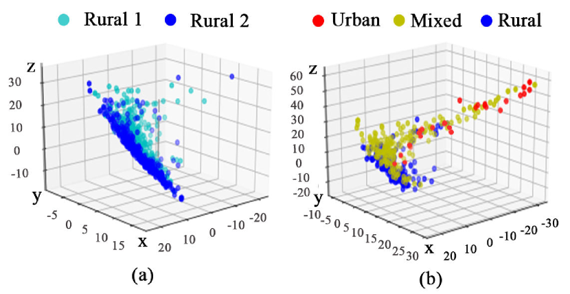
Figure 4: Embedding examples: (a) two rural areas show similar traits on the reduced dimensions; (b) semi-urban areas (marked as mixed) possess both traits of rural and urban areas.

Fig. 4 displays the feature vectors of the satellite images of five districts over a 3-dimensional space. Two rural districts appearing on the left-hand side exhibit a similar embedding space, whereas the three districts on the right-hand side exhibit different embedding spaces. Densely urbanized areas (red dots) have high variances ($y$-axis) and high mean values ($z$-axis) in the figure. In contrast, vast rural areas, which are denoted by blue or light blue dots, have comparatively low variances and low mean values ($z$-axis). The images on the right-hand side were chosen from a new district town that has a mixture of rural and urban areas and reports its embedded space in ‘mixed’ (yellow dots). The satellite images belonging to this mixed district indeed possess statistical characteristics intermediate between urban and rural. Similar to these examples, areas with distinct characteristics have different statistical values; thus, the summarized features can reflect the characteristics of districts.

Finally, cross-products of features were added to consider interactions to enrich the information regarding unknown embedded space distributions. These complete sets of features were learned per district $i$, as illustrated in the bottom part of Fig. 2 and became a fixed-sized representation $\mathbf{r}_{i}$. To predict the $y_{i}$ value for district $i$, we used $\mathbf{r}_{i}$ to fit a regressor.

Data

This study utilizes the following data: regional-level demographics and high-resolution satellite imagery. Both data types from many developed countries are accessible via the REST APIs of Esri®ArcGIS, a famous repository of maps and geographic (?). We chose South Korea as a representative developed country for training the model. Then, among all available satellite images of South Korea, we further identified those in which at least three vertices of an image tile belong to the polygon representing the boundaries of each district, as illustrated in Fig. 1. This heuristic is simple but reasonable for addressing various polygon shapes. In total, 96,131 satellite images (256x256 pixels) of 230 South Korean districts were collected in this manner. The utilization of all image tiles per district distinguishes our work from those of others, c.f., previous studies used a fixed set of satellite images; – for example, a seminal study conducted in African countries used 100 randomly chosen images tiles over 10x10$km^{2}$ areas (?).

Satellite imagery data

The World Imagery satellite data captured by DigitalGlobe provides 256x256-pixel image tiles over a wide range of zoom levels, $Z$ (0$\sim$18). While a single increment in the zoom level enlarges the area within both the vertical and horizontal directions, the overall number of pixels maintains the same size. Hence, the resolution becomes double, and the coverage becomes quarter per increment.

The highest freely available resolution is 0.6m-resolution, which is $Z$=18. However, under such resolution, image annotation becomes challenging because of the small spatial coverage of each image tile. Moreover, the size of district data increases exponentially, leading to computation overhead in training the model. In contrast, choosing a zoom level below 15 results in poor performance because one image tile may contain multiple districts. The smallest district in data spans 2.8$km^{2}$, which cannot be distinguished at a zoom level 14. We chose the zoom level of 15 with 4.7m-resolution, which allows for the identification of large objects that cover more than 5x5$m^{2}$. For example, we can start to recognize buildings and roads but not the cars on the street at $Z$=15. Each image covers approximately 1.4$km^{2}$, which is considered appropriate for observing human settlements in the previous research (?) using a satellite image of coverage 1$km^{2}$.

Table 1: Example of demographic attributes

Category	Variable ID	Description
Population	density	Population per square kilometer
Age	0-14	Population density by age 0-14
	15-29	Population density by age 15-29
	30-44	Population density by age 30-44
	45-59	Population density by age 45-59
	60+	Population density by age 60+
Education	nodegree	Population density by no degree
	elementary	Population density by elementary school
	middle	Population density by middle school
	…	…
	phd	Population density by Ph.D. degree
Household	count	Household count per square kilometer
	size	Average household size
Income	total	Total purchasing power per household
	capita	Purchasing power per capita

Demographics data

The Esri Demographics by Michael Bauer Research GmbH provides 2018 demographics data and the boundary polygon shapes of districts in 135 countries. For South Korea, the following data types were available: Population, Age, Education, Household, and Income. The population density and 27 other demographics measured per capita were used as representative ground truth data in this paper. Table 1 displays example demographic fields and their descriptions.

Results

Performance evaluation and ablation study

We conduct a set of experiments. The first evaluation takes advantage of the population demographics by dividing these data into a training set and a test set in an 80%–20% ratio. 4-fold cross-validation is applied to the training data set to tune the model’s hyperparameters, such as the PCA dimensions and the regularization term in the cost function.

We implemented nine baselines to evaluate. Nightlight uses the total light intensity of the districts from nighttime satellite imagery to predict economic scales (?). A regressor was built and trained to obtain the sum of nightlights in each district. Then, Auto-Encoder extracts compact features as step2 on our model. An autoencoder is an unsupervised deep learning algorithm that does not need any label information. The model aims to learn an approximate identity function to construct an output that is similar to the input while limiting the number of hidden layers. No-Proxy is identical to the proposed model but lacks any knowledge transfer from the proxy dataset. This model was pretrained only with the ImageNet dataset and, hence, can demonstrate the value of the custom dataset.

To verify the effectiveness of READ compared to a well-known model (?), we trained JMOP (Jean Model with Our Proxy) which is a combination of two models. First, we use a proxy which is predicting for rural, urban, and inhabited classes in the same method of READ. Then, we summarize the features and use them to predict with an identical set of model (?). Finally, SOTA is the best known grid-based approach for population density prediction (?). The implementation details of this model are not published, but the prediction results on each arc-second block (approximately 30x30$m^{2}$) are shared online. We could aggregate the published grid-level data across districts and regress such data with ground truth statistics. The four remaining baselines are ablation studies that remove each feature from READ.

Table 2: Baseline results and ablation study. Performance comparison on predicting population density by READ and nine baselines.

Model	MSE	R-Squared
Nightlight	0.4254$\pm$0.0664	0.6133$\pm$0.0635
Auto-Encoder	1.6242$\pm$0.3445	0.6347$\pm$0.0823
No-Proxy	0.2800$\pm$0.1118	0.7359$\pm$0.1117
JMOP	0.4448$\pm$0.0998	0.8985$\pm$0.0253
SOTA	-	0.9231
READ w/o $\mu$	0.2612$\pm$0.0632	0.9429$\pm$0.0155
READ w/o $\rho$	0.2165$\pm$0.0596	0.9527$\pm$0.0140
READ w/o $n$	0.1921$\pm$0.0471	0.9579$\pm$0.0119
READ w/o $\sigma$	0.1902$\pm$0.0592	0.9586$\pm$0.0130
READ	0.1761$\pm$0.0383	0.9617$\pm$0.0090

All models were trained with an 80%-20% train-test ratio and 4-fold cross-validation. XGBoost (?) was used to enhance prediction accuracy. The models were evaluated 20 times with a randomly split dataset. Table 2 reports the mean and standard deviation of the prediction performances. READ outperforms all of the nine baselines in both the R-squared ($R^{2}$) and mean squared error (MSE) values. Our model even outperforms the current state-of-the-art (SOTA) approach, which is (?). We find that transfer learning from the custom labeled dataset helps produce a more meaningful embedded, by distilling knowledge associated with urban and rural classifications. This finding is demonstrated by the increased prediction quality against two models: No-Proxy and Auto-Encoder. Furthermore, the quality gain over JMOP indicates that the summarizing technique of READ contributes massively to the performance gain. The ablation study shows that removing any of the descriptive statistics lowered the performance, indicating that $n$, $\mu$, $\rho$, and $\sigma$ all make a meaningful contribution.

Comparisons of architecture alternatives

Subsequently, we tested alternative design choices. First, we considered the following networks as the backbone CNNs: 1) DenseNet121, a densely connected convolutional network that connects each layer to each other layer in a feed-forward fashion (?); 2) AlexNet, an 8 layer network that won the ImageNet challenge 2012 (?); and 3) VGG16, a 16 layer very deep convolutional network (?). These options were compared to our choice of ResNet18 (?). Using ResNet18 as the backbone CNN was found to yield the highest $R^{2}$ value, which is demonstrated in Table 3. The difference, however, remains in the range between 0.021 and 0.0253.

Table 3: Comparison across different backbone networks.

Model	ResNet18	DenseNet121	AlexNet	VGG16
$R^{2}$	0.9617	0.9337	0.9364	0.9407

We also apply the following regressors: 1) XGBoost (?); 2) Ridge and Lasso as linear models with different regularization terms; 3) Random Forest (RFT) as a widely used ensemble model; and 4) Gradient Boosting Tree (GBT) as an ensemble model with boosting that nullifies overfitting. Fig. 5 shows the prediction accuracy as a function of the dimension size. The Lasso and Ridge regression showed a decreasing performance over the component count after four components in the case of Ridge and six components in the case of Lasso regression. These results are likely due to high dimensional input features and the lack of effective regularization in those models. In contrast to these methods, XGBoost, Random Forest, and Gradient Boosting Tree were resistant to overfitting, and XGBoost achieved the best performance in our model.

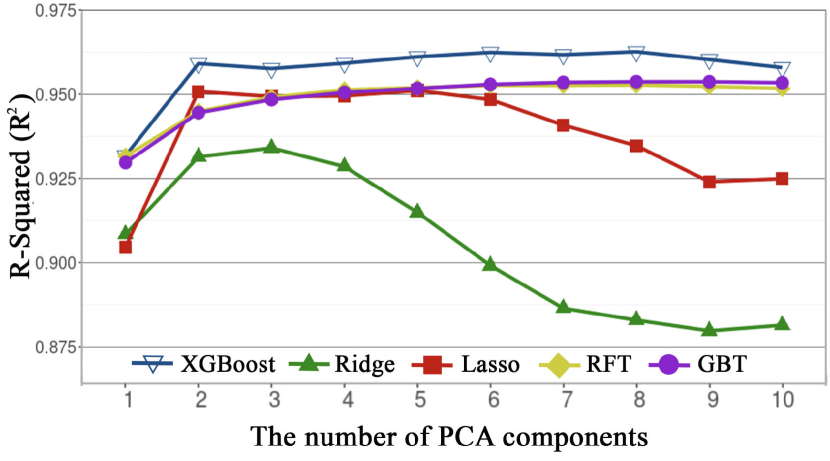
Figure 5: Prediction performances by the number of PCA components.

Evaluation over broader scales and countries

The final evaluation reports predictions of a complete set of economic scales by READ. All values are log-scaled, and XGBoost is used. The average $R^{2}$ of 20 trials of prediction of the study area is shown in Table 4. The third column represents READ applied to South Korea to predict the population density and its subclass divided by age very precisely ($R^{2}$ > 0.95). In the income category, the purchasing power per capita (capita) is predicted by $R^{2}$ as 0.7603. Finally, two demographics in the household category show an extreme difference in their prediction quality. While the household count per square kilometer (count) reports the highest $R^{2}$ of 0.9664, the average household size (size) reports the lowest $R^{2}$, i.e., 0.6181, among the economic scales.

Table 4: Prediction performances of economic scales for South Korea and Vietnam.

Category	Variable ID	South Korea	Vietnam
Population	density	0.9617	0.8863
Age	0-14	0.9520	0.8756
	15-29	0.9570	0.8791
	30-44	0.9575	0.8881
	45-59	0.9624	0.8804
	60+	0.9654	0.8731
Household	count	0.9664	0.8896
	size	0.6181	0.4460
Income	capita	0.7603	0.6822

The high prediction capability of READ may be due to the custom dataset, which was built from the same country (see step1 in Fig. 2). To test its applicability, we gathered a total of 226,305 satellite images along with economic scale data from another country, Vietnam. Then, we applied the model learned from South Korea to predict the economic scales of Vietnam. Surprisingly, READ achieved a high $R^{2}$ value of 0.8863 in predicting the population density in Vietnam, even when it was trained solely on data from a different country.

The above finding demonstrates that the learned spatial representation of READ successfully captures general indicators of socioeconomic scales that extend beyond a single country use. It may be that Asian countries exhibit similar pathways in economic growth and demographic transition (?). Interestingly, we also note a substantial difference in the prediction quality of specific demographic attributes between the two countries. For example, the highest $R^{2}$ value in the age category is found in the ‘60+’ group in South Korea (0.9654) but in the ‘30-44’ group in Vietnam (0.8881), which might have been affected by the concentration of the elderly population in rural areas in South Korea due to demographic transition and rural-urban migration. In contrast, a more substantial younger population is known to live in rural areas in Vietnam (?), compared to South Korea.

Finally, as another way to quantify how much gain building a custom labeled dataset of land covers contribute to the model, we conducted another experiment. We additionally built a custom labeled dataset for Vietnam by hiring two local annotators and obtained the land cover labels for 1,000 randomly selected images. We used this customized dataset to retrain the entire model. However, building a customized dataset for Vietnam only led to a marginal gain in predictions. The prediction of population density improved to the $R^{2}$ value of 0.8876. We expect that the minimal performance gain from building a custom dataset for Vietnam data is due to the quality of satellite images. Unlike in the case of South Korea, many satellite images of the region available from ArcGIS contained clouds, even after applying a cloud filter.

Discussion & Conclusion

This paper proposed a novel model that efficiently limits the number of dimensions via transfer learning to summarize any number of satellite images. The final spatial representation, which is a fixed-length embedded vector, can be used to estimate the socioeconomic growth of urban and rural areas at the district level. This method could benefit developing countries lacking the much-needed infrastructure to monitor their rapid urbanization process closely. Utilizing all of the high-resolution daytime satellite images, without restraining the model to handle random samples as in previous work, led to the substantial performance gain. Our approach can be widely applied by national and regional governments to estimate economic scales, such as the age and purchasing of district-level populations. Below, we discuss two potential application domains of READ.

Revealing sub-district level scales

While we present the results of district-level predictions, the proposed method predicts attributes over smaller levels, i.e., satellite image tiles. The potential to utilize such micro-level inference is magnificent. READ not only distinguishes urban and rural areas, as demonstrated in Fig.6, but also captures the fine-grained layout of land cover. The rural area depicted in the figure indicates that the degree of urbanization is not even across the district and that the regions illustrated in white color, in particular, lack urban infrastructure. Such fine-grained demographic information could be highly valuable in helping answer questions, such as “which areas of the city are growing the fastest or the slowest?” and “which areas outside the city lack critical infrastructure, such as roads?” that could have been answered, otherwise, via expensive offline surveys. Our technique, READ, can sufficiently summarize the high-resolution satellite imagery to benefit neighborhood-level demographic research.

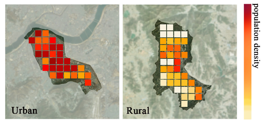
Figure 6: A single district often comprises multiple neighborhoods of different economic scales. READ naturally models such small-scale variations.

Application to measure urban sprawl

Cities are overgrowing worldwide, and this urbanization process is sometimes faster than the development of the necessary infrastructure needed for the urban population. This problem of tracking rapid urban growth, which is called urban sprawl (?), has been challenging due to the lack of data, particularly in rapidly evolving developing countries. We show with an example that applying READ over historical data can help better understand urban sprawls.

Fig. 7 displays the embedded feature vectors of satellite images on the reduced dimensions of one district at different times over a 3-dimensional space. By comparing the embedded feature vectors of the same region in (a) 2010, (b) 2015, and (c) 2018, we observe different types of vector space. The densely urbanized area (c) is diffusing in the $x$-axis direction. However, the less developed area (a) is spreading along the $z$-axis. Our finding indicates the change in a particular area that is relatively fast-growing over time. Detecting the changes in a specific region is recognized as an essential aspect of implementing policy to improve the quality of the local economic activity.

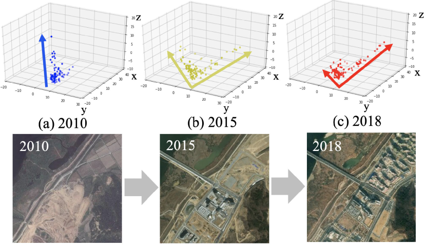
Figure 7: READ can be used to compare the evolution of the same district over multiple years. This given district exhibited mostly rural features in 2010, but its visual composition changed to contain a mix of urban and rural features towards 2018.

Limitations & Future work

This work has several limitations. First, the application of our model will be affected by the urbanization patterns and the quality of satellite imagery. Although we confirmed a high $R^{2}$ value in Vietnam for the model trained from South Korea data, such high applicability may be due to both countries showing similar patterns of urbanization, particularly in terms of building shapes (?). The architectural similarity may have contributed to the consistent performance over a new country, even though the model was solely trained using another country’s data. Nonetheless, we emphasize that land cover labels considered in the current paper (i.e., rural, urban, and uninhabited) are general. The model, therefore, is not specific to describing particular regional characteristics such as agriculture or mining. In the future, we plan to consider other benchmark data from vastly different cultural backgrounds. Second, our model utilizes only freely available data. Currently, rich geospatial data describing the elevation of surfaces such as buildings, vegetation, and other human artifacts, are becoming available, e.g., the Digital Surface Model (DSM) data. While DSM data is costly to obtain, future studies may incorporate alternative datasets to advance characterizing urban agglomerations further. Finally, our approach lacks interpretability. Due to the black-box nature of the deep learning model utilized, the model cannot determine which image feature most contributes to urbanization. We aim to enhance interpretability by adopting explainable structures, such as grad-CAM (?).

References

- [Bagan and Yamagata 2015] Bagan, H., and Yamagata, Y. 2015. Analysis of urban growth and estimating population density using satellite images of nighttime lights and land-use and population data. GIScience & Remote Sensing 52(6):765–780.
- [Bharti et al. 2011] Bharti, N.; Tatem, A. J.; Ferrari, M. J.; Grais, R. F.; Djibo, A.; and Grenfell, B. T. 2011. Explaining seasonal fluctuations of measles in niger using nighttime lights imagery. Science 334(6061):1424–1427.
- [Chaturvedi, Ghosh, and Bhandari 2011] Chaturvedi, M.; Ghosh, T.; and Bhandari, L. 2011. Assessing income distribution at the district level for india using nighttime satellite imagery. proc. of the APAN.
- [Chen and Guestrin 2016] Chen, T., and Guestrin, C. 2016. Xgboost: A scalable tree boosting system. In proc. of the ACM SIGKDD.
- [Chen and Nordhaus 2011] Chen, X., and Nordhaus, W. D. 2011. Using luminosity data as a proxy for economic statistics. PNAS 108(21):8589–8594.
- [CIESIN 2016] CIESIN, C. U. 2016. Documentation for the gridded population of the world. Available at http://dx.doi.org/10.7927/H4D50JX4. Date accessed 05 Sep 2019.
- [Deng et al. 2009] Deng, J.; Dong, W.; Socher, R.; Li, L.-J.; Li, K.; and Fei-Fei, L. 2009. Imagenet: A large-scale hierarchical image database. In proc. of the IEEE CVPR.
- [Doll, Muller, and Morley 2006] Doll, C. N.; Muller, J.-P.; and Morley, J. G. 2006. Mapping regional economic activity from night-time light satellite imagery. Ecological Economics 57(1):75–92.
- [Doupe et al. 2016] Doupe, P.; Bruzelius, E.; Faghmous, J.; and Ruchman, S. G. 2016. Equitable development through deep learning: The case of sub-national population density estimation. In proc. of the ACM DEV.
- [Doxsey-Whitfield et al. 2015] Doxsey-Whitfield, E.; MacManus, K.; Adamo, S. B.; Pistolesi, L.; Squires, J.; Borkovska, O.; and Baptista, S. R. 2015. Taking advantage of the improved availability of census data: a first look at the gridded population of the world, version 4. Papers in Applied Geography 1(3):226–234.
- [Elvidge et al. 2009] Elvidge, C. D.; Sutton, P. C.; Ghosh, T.; Tuttle, B. T.; Baugh, K. E.; Bhaduri, B.; and Bright, E. 2009. A global poverty map derived from satellite data. Computers & Geosciences 35(8):1652–1660.
- [Ewing, Pendall, and Chen 2002] Ewing, R.; Pendall, R.; and Chen, D. 2002. Measuring sprawl and its impacts: the character and consequences of metropolitan expansion. Washington DC: Smart Growth America.
- [Foley et al. 2005] Foley, J. A.; DeFries, R.; Asner, G. P.; Barford, C.; Bonan, G.; Carpenter, S. R.; Chapin, F. S.; Coe, M. T.; Daily, G. C.; Gibbs, H. K.; et al. 2005. Global consequences of land use. Science 309(5734):570–574.
- [Ghosh et al. 2013] Ghosh, T.; Anderson, S.; Elvidge, C.; and Sutton, P. 2013. Using nighttime satellite imagery as a proxy measure of human well-being. Sustainability 5(12):4988–5019.
- [He et al. 2016] He, K.; Zhang, X.; Ren, S.; and Sun, J. 2016. Deep residual learning for image recognition. In proc. of the IEEE CVPR.
- [Hochreiter and Schmidhuber 1997] Hochreiter, S., and Schmidhuber, J. 1997. Long short-term memory. Neural computation 9(8):1735–1780.
- [Hu and Huang 2019] Hu, T., and Huang, X. 2019. A novel locally adaptive method for modeling the spatiotemporal dynamics of global electric power consumption based on dmsp-ols nighttime stable light data. Applied Energy 240:778–792.
- [Huang et al. 2017] Huang, G.; Liu, Z.; Van Der Maaten, L.; and Weinberger, K. Q. 2017. Densely connected convolutional networks. In proc. of the IEEE CVPR.
- [Iimi 2005] Iimi, A. 2005. Urbanization and development of infrastructure in the east asian region. JBICI Review 10(1):88–109.
- [Jean et al. 2016] Jean, N.; Burke, M.; Xie, M.; Davis, W. M.; Lobell, D. B.; and Ermon, S. 2016. Combining satellite imagery and machine learning to predict poverty. Science 353(6301):790–794.
- [Johnston et al. 2001] Johnston, K.; Ver Hoef, J. M.; Krivoruchko, K.; and Lucas, N. 2001. Using ArcGIS geostatistical analyst, volume 380. Esri Redlands.
- [Krizhevsky, Sutskever, and Hinton 2012] Krizhevsky, A.; Sutskever, I.; and Hinton, G. E. 2012. Imagenet classification with deep convolutional neural networks. In proc. of the NIPS.
- [Lab and Center for International Earth Science Information Network 2019] Lab, F. C., and Center for International Earth Science Information Network, C. C. U. 2019. Data for Good program. Available at https://data.humdata.org/organization/facebook. Date accessed 05 Sep 2019.
- [Letu et al. 2011] Letu, H.; Tana, G.; Hara, M.; and Nishio, F. 2011. Monitoring the electric power consumption by lighting from dmsp/ols nighttime satellite imagery. In prof. of the IEEE International Geoscience and Remote Sensing Symposium.
- [McNicoll 2006] McNicoll, G. 2006. Policy lessons of the east asian demographic transition. Population and Development Review 32(1):1–25.
- [Oliver et al. 2018] Oliver, A.; Odena, A.; Raffel, C. A.; Cubuk, E. D.; and Goodfellow, I. 2018. Realistic evaluation of deep semi-supervised learning algorithms. In proc. of the NIPS.
- [Pandey, Agarwal, and Krishnan 2018] Pandey, S. M.; Agarwal, T.; and Krishnan, N. C. 2018. Multi-task deep learning for predicting poverty from satellite images. In proc. of the AAAI.
- [Robinson, Hohman, and Dilkina 2017] Robinson, C.; Hohman, F.; and Dilkina, B. 2017. A deep learning approach for population estimation from satellite imagery. In proc. of the ACM SIGSPATIAL Workshop on Geospatial Humanities.
- [Selvaraju et al. 2017] Selvaraju, R. R.; Cogswell, M.; Das, A.; Vedantam, R.; Parikh, D.; and Batra, D. 2017. Grad-cam: Visual explanations from deep networks via gradient-based localization. In Proceedings of the IEEE International Conference on Computer Vision, 618–626.
- [Simonyan and Zisserman 2014] Simonyan, K., and Zisserman, A. 2014. Very deep convolutional networks for large-scale image recognition. arXiv preprint arXiv:1409.1556.
- [Simonyan and Zisserman 2015] Simonyan, K., and Zisserman, A. 2015. Very deep convolutional networks for large-scale image recognition. In proc. of the ICLR.
- [Sutton et al. 1997] Sutton, P.; Roberts, D.; Elvidge, C.; and Meij, H. 1997. A comparison of nighttime satellite imagery and population density for the continental united states. Photogrammetric Engineering and Remote Sensing 63(11):1303–1313.
- [Sutton et al. 2007] Sutton, P. C.; Elvidge, C. D.; Ghosh, T.; et al. 2007. Estimation of gross domestic product at sub-national scales using nighttime satellite imagery. International Journal of Ecological Economics & Statistics 8(S07):5–21.
- [Tarvainen and Valpola 2017] Tarvainen, A., and Valpola, H. 2017. Mean teachers are better role models: Weight-averaged consistency targets improve semi-supervised deep learning results. In proc. of the NIPS.
- [UNdata 2019] UNdata. 2019. Social indicators. Available at http://data.un.org. Date accessed 05 Sep 2019.
- [Vogel et al. 2018] Vogel, K. B.; Goldblatt, R.; Hanson, G. H.; and Khandelwal, A. K. 2018. Detecting urban markets with satellite imagery: an application to india. Technical report, National Bureau of Economic Research.
- [Xiao et al. 2015] Xiao, T.; Xia, T.; Yang, Y.; Huang, C.; and Wang, X. 2015. Learning from massive noisy labeled data for image classification. In proc. of the IEEE CVPR.
- [Xie and Weng 2016] Xie, Y., and Weng, Q. 2016. World energy consumption pattern as revealed by dmsp-ols nighttime light imagery. GIScience & Remote Sensing 53(2):265–282.
- [Xie et al. 2016] Xie, M.; Jean, N.; Burke, M.; Lobell, D.; and Ermon, S. 2016. Transfer learning from deep features for remote sensing and poverty mapping. In proc. of the AAAI.
- [Yang et al. 2016] Yang, Z.; Yang, D.; Dyer, C.; He, X.; Smola, A.; and Hovy, E. 2016. Hierarchical attention networks for document classification. In proc. of the NAACL-HLT.
- [Yosinski et al. 2014] Yosinski, J.; Clune, J.; Bengio, Y.; and Lipson, H. 2014. How transferable are features in deep neural networks? In proc. of the NIPS.