First-Passage Percolation under extreme disorder: from bond-percolation to Kardar-Parisi-Zhang universality

Abstract

We consider the statistical properties of arrival times and balls on first-passage percolation (FPP) $2D$ square lattices with strong disorder in the link-times. A previous work showed a crossover in the weak disorder regime, between Gaussian and Kardar-Parisi-Zhang (KPZ) universality, with the crossover length decreasing as the noise amplitude grows. On the other hand, this work presents a very different behavior in the strong-disorder regime. A new crossover length appears below which the model is described by bond-percolation universality class. This characteristic length scale grows with the noise amplitude and diverges at the infinite-disorder limit. We provide a thorough characterization of the bond-percolation phase, reproducing its associated critical exponents through a careful scaling analysis of the balls. This is carried out through to a continuous mapping of the FPP passage time into the occupation probability of the bond-percolation problem. Moreover, the crossover length can be explained merely in terms of properties of the link-time distribution. The interplay between the new characteristic length and the correlation length intrinsic to bond-percolation determines the crossover between the initial percolation-like growth and theasymptotic KPZ scaling.

I Introduction

Geometry on random manifolds presents both applied and fundamental interest, with applications ranging from the physics of polymers and membranes Nelson ; Boal to quantum gravity Itzykson_Drouffe ; Booss.book ; Ambjorn_97 . Specifically, geodesics and isochrones on random manifolds, corresponding to non-Euclidean versions of straight lines and circumferences, present a very rich behavior Santalla_15 ; Santalla_17 . It was recently shown that, in the case of random surfaces which are flat in average and with short-range correlations in the curvature, geodesics present fractal structure, governed by exponents corresponding to the celebrated Kardar-Parisi-Zhang (KPZ) universality class Kardar_86 describing random interfacial growth Barabasi ; Krug_97 ; Krug_10 ; Halpin_15 . Specifically, the lateral deviation of a geodesic joining two points separated an Euclidean distance $L$ scales like $L^{1/z}$, where $z=3/2$ is the dynamical exponent of KPZ. Moreover, the deviation of the arrival times scales like $L^{\beta}$, with $\beta=1/3$, and their fluctuations follow the Tracy-Widom distribution for the lowest eigenvalues of random unitary matrices Praehofer_02 ; Takeuchi_11 ; Corwin_13 .

When the manifold is discretized the problem is called first-passage percolation (FPP) Hammersley_65 ; Howard_04 ; Auffinger_17 . Given an undirected lattice, e.g. $\mathbb{Z}^{2}$, a randomly chosen link-time $t$ is assigned to each edge between neighboring nodes. Link-times are independent and identically distributed (i.i.d.) random variables with common probability density function $f(t)$ and cumulative distribution function $F(t)$. Notice that for the model to present the structure of a metric space we must assume $F(0)=0$. This problem bears a strong relation with the directed polymers in random media (DPRM) Kardar_87 ; Krug_91 ; Halpin_95 , where we are asked to find the minimal energy configuration for a polymer of fixed length on a random surface. The most relevant difference between them is the fixed length constraint, which does not hold for geodesics. FPP results have been successfully applied to magnetism Abraham_95 , wireless communications Beyme_14 , ecological competition Kordzhakia_05 and molecular biology Bundschuh_00 .

The main objects of study in FPP are geodesics, i.e. minimal time paths joining pairs of points, and balls $B(T)$ given by the set of nodes which can be reached from the origin in a time less than $T$. There are some rigorously proved results, such as the Galilean invariance, $z(1+\beta)=2$ Chatterjee_13 . It has also been proven (shape theorem) that, when the lattice structure is properly smoothed out, the ball $B(T)$ grows linearly with $T$ and has an asymptotic shape $B_{0}$ which is non-random. Moreover, for suitable conditions on the moments of $F$, $B_{0}$ is a convex set with nonempty interior and it is either compact or equals all of $\mathbb{R}^{d}$ (see Kesten_87 and references therein).

FPP presents a whole new set of features over the continuous version of the problem, such as a direction-dependent crossover associated with the so-called geodesic degeneracy Cordoba_18 , i.e. the number and structure of the geodesics joining two points in absence of noise. A characteristic length $d_{c}$ was found both in the square lattice and in random Delaunay triangulations, determining a crossover between Gaussian and KPZ behavior. This crossover length decreases as the noise amplitude increases following $d_{c}\sim({\rm CV})^{-2}$, where CV is the coefficient of variation of the link-time distribution, defined as ${\rm CV}\equiv s/\tau$, where $\tau$ and $s$ are respectively the mean value and deviation of the link-times Cordoba_18 . Those results are only valid when $d_{c}>1$, i.e. for $\tau>s$ or, in other terms, in the weak-disorder regime. For example, all uniform noise distributions fall into this regime.

Yet, for a strong noise, i.e. $s\gg\tau$, the characteristic length $d_{c}<1$ can not play the same role. In some relevant cases, $s$ and $\tau$ might even be ill-defined. Indeed, in the strong-disorder regime, link-times encompass several orders of magnitude. A limit case is given by the Bernoulli distribution, in which link-times can be zero with probability $p=F(0)$. If we identify now zero-time links with open bonds in a connected lattice we are effectively mapping our system to a problem of bond-percolation Kesten_87 ; Halpin_95 ; Stauffer_03 . Thus, critical FPP is defined by condition $F(0)=p_{c}$ Damron_17 ; Damron_19 ; Yao_18 ; Kesten_97 ; Yao_14 and supercritical FPP is defined by $F(0)>p_{c}$ Zhang_95 ; Garet_07 ; Yao_13 , where $p_{c}$ is the critical probability in bond-percolation Stauffer_03 . For $F(0)\geq p_{c}$ there exists an infinite connected set of edges with zero crossing-time so that traveling across this infinite cluster costs no time Aizenman_87 . As a consequence, the route between two lattice nodes will always stay within the infinite cluster except for a few edges Zhang_95 . Furthermore, it has been shown that the asymptotic shape $B_{0}$ equals all of $\mathbb{R}^{d}$ if and only if $F(0)\geq p_{c}$ Kesten_86 ; Chayes_86 .

Much effort in critical FPP has been devoted to the analytical study of the time constant $\mu$, defined as the limit of the passage time to a site (or to some boundary) normalized by its distance from the origin, as the distance goes to infinity. This limit has been proven to exist for suitable conditions on the moments of $F$ Smythe_78 , and $\mu=0$ if and only if $F(0)\geq p_{c}$ Kesten_87 . Indeed, the existence of large clusters with zero-weight edges leads to a passage time that grows at most logarithmically with distance, yielding a zero time constant Damron_19 ; Yao_18 ; Damron_17 . The work has focused on the characterization of the asymptotics of this arrival time by conditions on the distribution function $F$ Damron_17 ; Damron_19 ; Yao_18 ; Kesten_97 ; Yao_14 , yielding relevant results such as a universal expression for the time constant on $2D$ lattices Damron_19 , the proposition of a central limit theorem for the passage time Yao_18 ; Kesten_97 or a relation between critical FPP and invasion percolation Damron_17 .

The geometry of the minimal paths has also been a matter of study Giles_19 . In the early 80’s, Ritzenberg and Cohen considered shortest paths on a percolation cluster beyond criticality, i.e. spanning an infinite number of nodes Ritzenberg_84 , computing their fractal dimension. Kerstein and coworkers considered FPP with two possible link-times, a slow one and a (extremely) fast one Kerstein_85 ; Kerstein_85b ; Kerstein_86 . As the density of slow links increases, they describe a crossover from chemical to contact propagation. Chemical propagation describes geodesics that only employ fast links, while contact propagation refers to the use of slow links to jump from cluster to cluster. In the first case, the conduction rate is limited by the geodesic tortuosity, i.e. the average number of links along a typical fast path. For contact propagation, on the other hand, the conduction rate is limited by the ratio of slow bonds. The crossover between both regimes takes place at the percolation threshold. Geodesics on critical and super-critical percolation clusters were studied by several authors Zhang_95 ; Garet_07 ; Yao_13 ; Damron_17 ; Yao_18 ; Garet_10 , and a correspondence between geodesics on critical percolation clusters and Schramm-Loewner evolution curves has been recently put forward Pose_14 , lending support to the idea that they might be conformally invariant Di_Francesco .

In this article, we characterize the statistical properties of arrival times and balls on strongly disordered networks. Our purpose is to study the behavior of the model close to the critical case discussed so far, but keeping the condition $F(0)=0$ necessary for it to represent a metric space. We propose a mapping of the passage time into the probability $p$ of a bond being open, that allows us to map the FPP problem into a family of bond-percolation problems. Making use of detailed numerical simulations, we show how the scaling exponents of percolation theory map into those of the geodesic behavior below a certain crossover length, above which the geodesics attain the standard KPZ behavior. This new crossover length increases with the noise amplitude and seems to diverge for infinite noise, which leads us to conjecture that this limit might be related to the critical or supercritical FPP cases, depending on the link-time distribution.

This article is organized as follows. Section II presents the first-passage percolation model and our basic assumptions. Next, in section III we compare the statistical properties of the arrival times in the weak and strong disorder regimes. The mapping of the FPP problem into bond percolation is addressed in section IV, where we also present a comprehensive scaling analysis of the FPP balls that recovers the critical exponents of percolation. In section V we propose a model for the characteristic length that controls the extent of the percolation domain. Large scale behavior and the crossover towards standard KPZ scaling is described in Sec. VI, in which we also discuss the transition between the weak and strong disorder regimes. Section VII is devoted to a summary of our conclusions and our ideas regarding future work.

II Model and definitions

Let us consider a $L\times L$ square lattice (odd $L$), with nodes $\textbf{x}_{i}$ and a central node $\textbf{x}_{0}=(0,0)$. We assign a link-time $t(\textbf{x}_{i},\textbf{x}_{j})$ to each pair of nearest-neighbor nodes, $\textbf{x}_{i}$ and $\textbf{x}_{j}$. Given a path $\Gamma=\{\textbf{x}_{0},\textbf{x}_{1},\cdots,\textbf{x}_{m}\}$ joining the center to site $\textbf{x}_{m}$, in order to traverse that path we would need a time

$$T_{\Gamma}(\textbf{x}_{m})=\sum_{i=1}^{m}t(\textbf{x}_{i-1},\textbf{x}_{i}).$$ (1)

We define the arrival time as the minimal value over all paths reaching arbitrary node x from $\textbf{x}_{0}$:

$$T(\textbf{x})\equiv\min_{\Gamma}\{T_{\Gamma}(\textbf{x})\},$$ (2)

and the corresponding path is the geodesic or optimal path to that point. For a generic distribution of link-times the geodesic will be unique, but geodesic degeneracy can play an important role in some cases Cordoba_18 . Let us remark that arrival times can be efficiently obtained for all sites making use of Dijkstra’s algorithm. Finally, we also define the ball $B(T)$ as the set of nodes which can be reached in a time smaller than a certain value $T$.

We consider the case in which link-times are independent and identically distributed (i.i.d.) random variables with common probability density function $f(t)$ and cumulative distribution function $F(t)$, with the only constraint of positivity: $F(0)=0$. If they exist, the link-time distribution is characterized by a mean value $\tau$ and a variance $s^{2}$,

As discussed in the introduction, it has been shown Cordoba_18 that for weakly disordered distributions with $\tau>s$ (CV$<1$) there exists a crossover length given by $d_{c}=a(\tau/s)^{2}>1$, with the scale factor $a=O(1)$ depending on the geometrical properties of the lattice (e.g. $a\simeq 1/3$ for the square lattice), such that arrival times to sites along the axis at a distance $x\ll d_{c}$ follow Gaussian statistics, and KPZ statistics for $x\gg d_{c}$. Indeed, in that case the geodesic will not deviate from the straight line up to a distance $\sim d_{c}$. This behavior is expected to occur along the non-degenerate directions of regular lattices and also in low degeneration random lattices such as Delaunay triangulations Cordoba_18 . On the other hand, for disordered distributions with $\tau<s$ (CV$>1$) thus giving $d_{c}<1$ we enter the strong disorder regime, and the statistical properties of the arrival times change considerably.

Uniform link-time distributions have necessarily $d_{c}>1$ (note that CV$<3^{-1/2}$), but other distributions interpolate smoothly between these two regimes. That is the case of the three probability distributions employed in this work: Weibull (Wei$(\lambda,k)$), Pareto (Par$(t_{m},\alpha)$) and Log-Normal (LogN$(\mu,\sigma)$), whose definition and basic properties are listed in Appendix A. The three distributions are characterized by a shape parameter determining the amplitude of the noise: the power-law exponents $k$ and $\alpha$ in the Weibull and Pareto distributions respectively, and the variance $\sigma$ in the Log-Normal. As we show there, in all cases $d_{c}$ is a monotonic function of it, increasing for the first two cases and decreasing for the Log-Normal.

In order to unify our description we introduce the concept of order parameter to identify the distribution parameter which, when decreasing, makes the strength of disorder increase (by convention) in a monotonic way. We thus identity $k$, $\alpha$ and $\sigma^{-1}$ as the corresponding order parameters of the above distributions. For the sake of clarity we will denote this order parameter by $o$. As a result of this convention $d_{c}$ is an increasing monotonic function of $o$. We also introduce the symbol $o^{\star}$ to denote the value of the order parameter yielding $d_{c}=1$: $d_{c}(o^{\star})=1$. In other words, $o^{\star}$ determines the crossover point between the weak ($o>o^{\star}$ and $d_{c}>1$) and the strong ($o<o^{\star}$ and $d_{c}<1$) disorder regimes.

There is an interesting limit of the model which will be considered as a reference, the so-called homogeneous case in which link-times have uniform value $\tau_{0}$, and which corresponds to the delta distribution $f(t)=\delta(t-\tau_{0})$. As we show in Appendix A, the homogeneous case is obtained at the limit $o\rightarrow\infty$ (i.e. “infinite” order) of the above distributions (Eq. (35)).

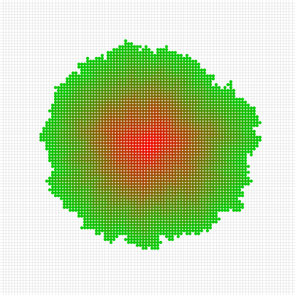
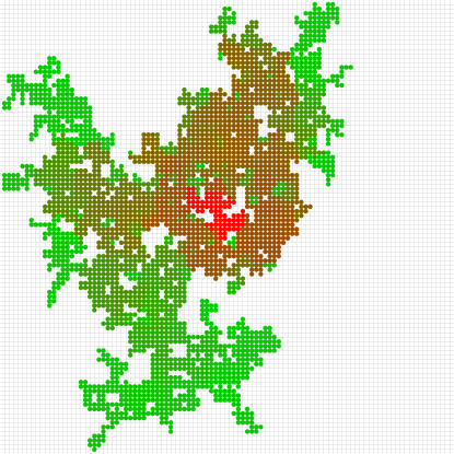
Figure 1: (Left) FPP ball corresponding to $T=25$ on a square lattice, for a link-time Weibull distribution Wei$(1,2)$. Colors are associated to different arrival times. (Right) FPP ball corresponding to $T=0.1$ when the link-times are drawn from Wei$(1,0.1)$. Notice that the crossover value of the order parameter is $k^{\star}\approx 1.79$.

Before going in-depth into the analysis of the model, it is worth having a look at the different behaviors at both sides of this divide. The left panel of Fig. 1 shows the FPP ball $B(T)$ obtained for $T=25$ on a $L=101$ lattice whose link-crossing times are drawn from a Weibull distribution with $k=2$, for which $d_{c}\approx 1.22$. The final ball appears rough, and indeed this roughness can be shown to correspond to the well-known KPZ universality class. Colors provide information about the arrival time to all sites within the ball, which we can see to behave in a reasonable smooth way. On the other hand, the right panel corresponds to $T=0.1$ for a distribution with $k=0.1$, for which $d_{c}\approx 2\cdot 10^{-6}$. Notice that the aspect of the ball is much less round, with abundance of cavities. Another salient feature is the sharpness of the color gradation. Instead of a smooth variation, we can determine clear boundaries within the ball.

III Fluctuations of the arrival times: from weak to strong disorder

Let us explore numerically the statistical properties of the arrival times using a $L\times L=2001\times 2001$ lattice and link-times drawn from the distributions presented above with different values of the order parameter, in order to interpolate smoothly from the weak to the strong-disorder regimes. Moreover, we will always average over $N=10^{4}$ samples, unless otherwise stated. As in Fig. 1, most of the results displayed hereafter will be obtained from the Weibull distribution, for which the crossover value of the order parameter is $o^{\star}=k^{\star}=1.79$ (Appendix A). Unless otherwise stated, it must be assumed that they hold for the other distributions. If results are distribution dependent we will address each distribution separately.

Let us consider the average arrival time in units of the average link-time, $\langle T\rangle/\tau$, for sites on the axis as a function of the distance to the center, $x=\|\textbf{x}\|$. In the weak disorder regime Cordoba_18 this magnitude grows linearly with the distance for $x\gg d_{c}$, with a slope that continuously decreases as the order parameter decreases. This slope represents the inverse of the normalized velocity of growth, closely related to the time constant $\mu$ discussed in the introduction. It is bounded from above by the trivial value obtained in the homogeneous case ($o\rightarrow\infty$): $1$ in the axis and $\sqrt{2}$ for the diagonal, leading to balls with diamond shapes. As the order parameter decreases the slopes found in all lattice directions decrease (velocity increases), and when $o$ approaches the crossover value $o^{\star}$ ($d_{c}\rightarrow 1$), they become equal, thus explaining the circular shape of the balls in average (see e.g. the ball shown in left panel of Fig. 1).

The top panel of Fig. 2 shows $\langle T\rangle/\tau$ when the link-times follow the Weibull distribution for $k=0.2$. The arrival time seems to approach a linear growth with distance giving a slope much smaller than one. For reasons that will become apparent soon, we have employed two different sample sizes: $N=10^{3}$ (black symbols) and $N=10^{4}$ (red symbols), which coincide perfectly. The lower panel of Fig. 2 shows the values of $\langle T\rangle/\tau$ as a function of the distance when the link-times are drawn from a much lower value of the order parameter $k=0.03$, i.e. deep in the strong-disorder regime ($k\ll k^{\star}$). In this case, the times of arrival appear scattered, without a clear dependence on the distance. Moreover, the data for $N=10^{3}$ (black) and $N=10^{4}$ (red) are statistically different. This fact suggests that arrival times in this regime are very difficult to sample, pointing to an extremely broad distribution.

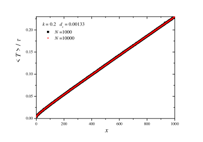
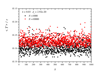
Figure 2: Average passage time, rescaled to the mean link-time $\tau$, to nodes at distance $x$ along the axis for the Weibull distribution with $k=0.2,$ (top) and $k=0.03$ (bottom). Results from two ensembles $N=1000$ and $N=10000$ have been represented in both cases with black and red symbols respectively.

To understand this behavior we have displayed in Fig. 3 the distribution of the arrival times to a given node x, denoted by $g_{\textbf{x}}(T)$. In the top panel we have considered a fixed position along the axis, $x=500$ and link-time distributions of the form Wei(1,$k$) for different values of $k$. The bottom part of Fig. 3 displays the results for the strongly disordered case with $k=0.03$ at different points along the axis.

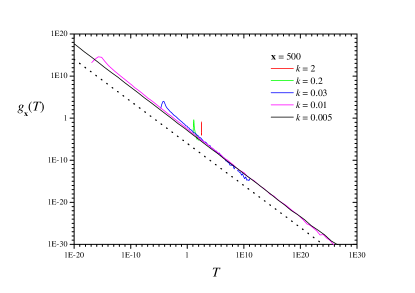
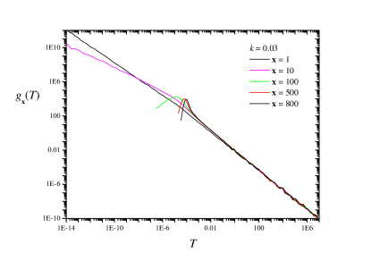
Figure 3: Histogram of passage time $T$ to: (top) site at distance $x=500$ in the axis for different values of $k$; (bottom) different sites along the axis for same $k=0.03$. Dotted line in top panel indicates the scaling $\sim T^{-1}$

In the weak-disorder regime, the distribution of arrival times at distance $x\gg d_{c}$ has been shown to follow the Tracy-Widom distribution for the Gaussian unitary ensemble (GUE) Praehofer_02 ; Takeuchi_11 ; Corwin_13 ; Cordoba_18 , which appears in the top panel of Fig. 3 (case $k=2$) in the form of a small and sharp peak (notice the log scale). However, as the disorder strength increases the distribution becomes right-skewed with the arrival time spanning an increasing range of orders of magnitude. There is still a well defined mode that moves towards smaller values and which is followed by a increasingly longer tail displaying a power-law scaling $\sim T^{-1}$ as $k\rightarrow 0$. As as consequence, for extreme disorder the mean arrival time is not well-defined and its average value is dominated by the largest value: $\langle T\rangle(\textbf{x})={1\over N}\sum_{i}^{N}T_{i}(\textbf{x})\simeq{1\over N}T_{\max N}(\textbf{x})$, where $T_{\max N}(\textbf{x})=\max_{i}\{T_{i}(\textbf{x})\}$, which certainly depends on the sample size thereby explaining the results displayed in Fig. 2 (bottom).

Let us now focus on the dependence of the passage-time distribution on distance for highly disperse distributions (case $k=0.03$, bottom panel of Fig. 3). We observe that the right tails of the skewed distributions merge into a single decay regardless of the position of the target point. This result, together with the max principle stated above, explain the independence of the average time $\langle T\rangle$ with distance displayed in Fig. 2 (bottom). Furthermore, as we move away from the center node, the distributions seem to approach a limit function which reveals that the minimum arrival time required to reach any lattice site is independent of its position. The existence of such minimal arrival time is an evidence of criticality in the model.

Another physical quantity of immediate interest in the study of the FPP model is the standard deviation of the arrival times. In the KPZ regime ($o>o^{\star}$ and for $x\gg d_{c}$) it scales as $\sigma_{T}\sim x^{\beta}$, with $\beta=1/3$, following the Family-Vicsek Ansatz. This standard deviation also corresponds to the roughness of the balls Santalla_15 and is analogous to the free energy fluctuations in directed polymers in random media (DPRM) Halpin_95 .

In Fig. 4 we have plotted the standard deviation of the arrival time $\sigma_{T}$, in units of the deviation of the link-time distribution, $s$, to nodes in the axis as a function of their distance $x$ to the center. In all cases, we are employing Weibull distributions Wei(1,$k$), for a range of values of $k$, which are shown along with the corresponding $d_{c}$. For $k>k^{\star}$ ($k=2$ up to $k=30$) we observe the well-known crossover from Gaussian towards KPZ scaling, with a behavior $\sigma_{T}\sim x^{1/2}$ for $d\ll d_{c}$ and $\sigma_{T}\sim x^{1/3}$ for $d\gg d_{c}$ Cordoba_18 . Moreover, for $x=1$ we have $\sigma_{T}/s\approx 1$, because the geodesic from a site to its neighbor usually consists of traversing the link joining them. On the other hand, we observe that for $k<k^{\star}$, $\sigma_{T}/s$ at $x=1$ is always below 1, and decreases very fast as $k\to 0$, implying that the geodesic between a site and its neighbor may be non-trivial. This fact suggests that geodesics in the strong-disorder regime can take long excursions in order to cover short distances on the lattice. Indeed, the geometric constraints imposed by the lattice are removed by the disorder, and the geodesics are never constrained to follow the axis (such as in the Gaussian regime for $k>k^{\star}$ and $x\ll d_{c}$) and explore the space freely in any direction.

Moreover, Fig. 4 shows that the KPZ regime, $\sigma_{T}\sim x^{1/3}$, is always recovered for distances above a new crossover length, $x\gg\ell_{o}$, with $\ell_{o}$ increasing as $k$ decreases. In the figure we have indicated with vertical segments and shadowed intervals theoretical estimates for the location of this crossover length according to the calculations that we present later. See Sec. VI for an explanation and discussion of these estimates.

A thorough explanation of the results presented in this section will be given in the following sections.

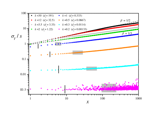
Figure 4: Standard deviation $\sigma_{T}$ of the arrival time to nodes at distance $x$ in the axis of the square lattice with link-times following a Wei(1,$k$) distribution, normalized to the standard deviation of the link-time distribution $s$. The corresponding values of $d_{c}$ are calculated from Eq. (36). Broken lines represent Gaussian pre-asymptotic growth ($\beta=1/2$) and KPZ scaling ($\beta=1/3$). Vertical segments in curves with $d_{c}<1$ ($k<k^{\star}$) indicate the value of length $\ell_{o}(T_{c})$ obtained from the chain model presented in Sec. V. Grey rectangles represent the interval $[\ell_{o}(T(p=0.99)),\ell_{o}(T(p=0.999))]$, as discussed in Sec. VI.

IV Mapping of FPP under extreme disorder into bond percolation

Strongly disordered link-time distributions lead to an interesting phenomenon: the arrival time, which is by definition the sum of all link-times along the geodesic path, is dominated by its largest term. Then, we can assert that

$$T(\textbf{x})=\min_{\Gamma}\sum_{i=1}^{m}t(\textbf{x}_{i-1},\textbf{x}_{i})\approx\min_{\Gamma}\left\{\max_{i}\{t(\textbf{x}_{i-1},\textbf{x}_{i})\}\right\},$$ (3)

i.e. arrival times follow a min-max principle. It is not hard to see that, if the max principle holds exactly, the set of points which can be reached in time $T$ corresponds to the set of points for which there is a path which never crosses a link with crossing-time larger (or equal) than $T$. Moreover, the perimeter of the ball will be surrounded by links with crossing times $t\geq T$. Thus, a clear connection with percolation can be established: the FPP ball obtained at time $T$, $B(T)$, corresponds to the cluster obtained in an equivalent bond percolation problem in which open bonds correspond to those FPP links with crossing-times lower than $T$, whereas closed bonds are given by the FPP links with crossing-time above $T$. To establish this equivalence we need to define the probability $p$ of a bond being open ($1-p$ of being closed). Under the assumption made in Eq. (3) this probability is given by the cumulative distribution function of the link-times evaluated at time $T$:

$$p=F(T)=\int_{0}^{T}f(t)\,dt.$$ (4)

This section is devoted to providing strong evidences that under extreme disorder conditions the FFP problem can be mapped into a bond-percolation problem through relation (4), which is the cornerstone of this work. Clearly the inverse transformation is given by $T=F^{-1}(p)$. For example, for the Weibull distribution we obtain:

$$p(T) =1-\exp\left(-(T/\lambda)^{k}\right),$$ (5)

$$T(p) =\lambda\left(-\ln\left[1-p\right]\right)^{1/k}.$$

Notice that $p(T)$ increases continuously with $T$ from $p(0)=0$ up to $p\rightarrow 1$ when $T\rightarrow\infty$. Also, the passage time corresponding to a given probability decreases monotonically as $k$ decreases, approaching $0$ as $k\rightarrow 0$.

We will show that FPP balls with arrival time under $T$ are equivalent to bond-percolation clusters obtained at bond probability $p=F(T)$. The mapping given in Eq. (4) will allow us to obtain some of the most relevant critical exponents of the associated percolation problem from the scaling analysis of the FPP geodesic balls. In the analysis we will use the standard notation of percolation theory Stauffer_03 . Since we are interested in the strong disorder regime we have to consider very low values of the order parameter $o\ll o^{\star}$. In the case of the Weibull distribution we shall focus on three values: $k=0.03$, $0.01$ and $0.005$, because they are sufficiently low to display the transition to the percolation phase at a reasonable computational cost (we recall that $k^{\star}\approx 1.79$).

IV.1 Ball size distribution

Percolation theory Stauffer_03 deals primarily with the statistical properties of the clusters of neighbouring sites which are occupied (site-percolation) or connected by open bonds (bond-percolation), when each site (or bond) is occupied (open) with a probability $p$. The critical point or percolation threshold $p_{c}$ is defined as the minimal probability $p$ for which an infinite percolation cluster is formed in an infinite lattice. Near the critical point the system is characterized by a set of critical exponents that are independent of the type of percolation or the lattice geometry, depending only on the dimension $D$ of the lattice. On the other hand, the percolation threshold varies with all these factors. For bond-percolation in a $D=2$ square lattice we have $p_{c}=1/2$.

Let $n_{s}(p)$ be the number of clusters of size $s$ (i.e. with $s$ sites), divided by the total number of lattice sites. This observable is known to present the following scaling relation near criticality ($p\rightarrow p_{c}$) and for large clusters ($s\rightarrow\infty$):

$$n_{s}(p)=s^{-\tau}g\left((p-p_{c})s^{\sigma}\right),$$ (6)

where $g(z)$ is a scaling function that approaches a constant value for $|z|\ll 1$ and decays exponentially for $|z|\gg 1$. This scaling relation introduces a crossover size $s_{\xi}$, which scales as $s_{\xi}\sim|p-p_{c}|^{-1/\sigma}$, such that:

$$n_{s}(p)\sim s^{-\tau}\quad{\rm for}\;\;s\ll s_{\xi}.$$ (7)

Beyond $s_{\xi}$, the power-law behavior fails and the number of clusters decays fast. In $2D$ we have $\tau=187/91$ and $\sigma=36/91$.

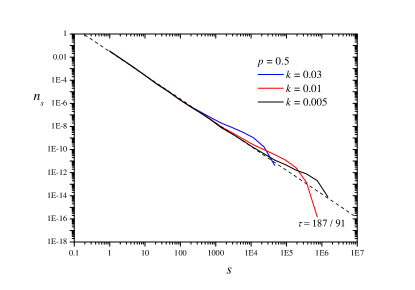
Figure 5: Ball size distribution, derived from the probability $W_{s}$ of obtaining a FPP ball with size $s$, using Eq. (8), for crossing-times following a distribution Wei(1,$k$) with $k=0.03$, $0.01$ and $0.05$, and for the arrival time $T$ which corresponds to $p=p_{c}=1/2$ according to Eq. (5). These arrival times are, respectively: $T=4.95\cdot 10^{-6}$, $T=1.21\cdot 10^{-16}$ and $T=1.46\cdot 10^{-32}$. The broken line indicates the scaling given in Eq. (7).

In a FPP framework we do not have access to this number of clusters. Yet, given a fixed arrival time $T$ we can estimate the probability that the FPP ball contains exactly $s$ sites, denoted here by $W_{s}(T)$. Since the center node always belongs to the FPP ball, this value can be mapped, in the percolation language, to the probability that a randomly chosen cluster site will be part of a cluster of size $s$. Let $w_{s}(p)$ be the probability (in the percolation problem) that the cluster to which a randomly chosen occupied site belongs has size $s$. It is easy to show that $n_{s}(p)=p\,w_{s}(p)/s$. We can now relate $W_{s}(T)$ and $w_{s}(p)$ through the mapping between arrival times and occupation probabilities given in Eq. (4), so we have $w_{s}(p(T))=W_{s}(T)$. Thus, for a given arrival time $T$, we propose that our FPP ball distribution is given by

$$n_{s}\left(p(T)\right)={p(T)\,W_{s}(T)\over s}.$$ (8)

Our analysis of the statistics of the FPP balls begins in Fig. 5, in which we show the ball size distribution calculated from Eq. (8) for the three distributions of reference and for arrival times corresponding to the critical probability $p_{c}=1/2$. We first observe a perfect collapse of the three curves into the scaling law given in Eq. (7) over several orders of magnitude. In bond percolation, the cutoff size $s_{\xi}$ diverges at $p_{c}$, so we should expect a continuous power-law decay. However, the plot shows that distributions deviate from the naively predicted scaling after a given point, showing first an increase with respect to the expected values leading to a final fast decay. Let us denote this cutoff size by $s_{o}(p)$, where we have assumed that, beyond its dependence on the order parameter $o$, it also depends on the probability $p$. It it clear that this crossover size increases as the disorder becomes stronger, which leads us to conjecture that it diverges as $o\rightarrow 0$ for any $p$.

The crossover size $s_{o}$ appears as a consequence of the breakdown of our main assumption: the max principle given in Eq. (3). Let us associate a length scale to $s_{o}$, given for example by the average radius of the balls of size $s_{o}$, and denote it by $\xi_{o}$. For length scales of the order of $\xi_{o}$ the geodesic paths are long enough to include links with crossing-times that, while smaller than the largest term, do significantly contribute to the arrival time. This means that, for a given arrival time $T$, not all the links with a crossing-time lower than $T$ are allowed, which leads to the breakdown of the max principle. As a result, the clusters with sizes larger than $s_{o}$ predicted by percolation theory are trimmed into FPP balls with smaller sizes, a fact that leads to the increase of $n_{s}$ for $s>s_{o}$ displayed in the figure. We will refer to this process as rounding-off. For larger length scales and thus longer geodesics ($s\gg s_{o}$), the round-off effect limits the size of the distributed balls at a given arrival time $T$ and the distribution drops steeply.

To see clearly this effect we can consider the critical point in bond percolation, where an infinite percolation cluster appears. Let us define the arrival time corresponding to the percolation threshold as the critical arrival time $T_{c}$: $T_{c}\equiv T(p_{c})$. For the Weibull distribution we obtain $T_{c}=\lambda(\ln 2)^{1/k}$. An infinite ball $B(T_{c})$ would necessarily imply infinitely long geodesics with an infinite number of links. Since link-times are positive we cannot observe an infinite ball for a finite arrival time. Only for distributions with $F(0)=p_{c}$ (critical FPP) or $F(0)>p_{c}$ (supercritical FPP) we observe infinite balls.

We can thus identify $\xi_{o}$ as the length scale characterizing the crossover observed in the model: for length scales much smaller than $\xi_{o}$ the behavior is the same as in bond percolation with $p=F(T)$.

At length scales of the order of $\xi_{o}$, we may postulate the existence of an equivalent bond-percolation problem characterized by an effective probability smaller than $p=F(T)$, because not all links with times below $T$ are allowed. The upper limit of the integral given in Eq. (4) can no longer be given by $T$, but by $T-\epsilon_{T}$ with some $\epsilon_{T}>0$. We conjecture that this results in an effective critical probability $p_{c,\text{eff}}$ which is slightly larger than the theoretical percolation threshold $p_{c}=1/2$. A rough argument for this is as follows. Let us consider the inverse problem and fix the occupation probability $p$ in the bond-percolation problem. Following the above reasoning we should expect that the effective arrival time $T_{\text{eff}}$ of the equivalent FPP problem should be of the form $T_{\text{eff}}(p)=T(p)+\epsilon_{T}(p)$, with $T(p)=F^{-1}(p)$ and some $\epsilon_{T}(p)>0$. At the critical point $p_{c}$ we can then write $T_{c,\text{eff}}(p_{c})=T(p_{c})+\epsilon_{T}(p_{c})=T_{c}+\epsilon_{T}(p_{c})$. We can now define the effective critical probability $p_{c,\text{eff}}$ as the probability that satisfies $T(p_{c,\text{eff}})=T_{c,\text{eff}}(p_{c})$. We then have $p_{c,\text{eff}}=F(T_{c,\text{eff}}(p_{c}))=\int_{0}^{T_{c,\text{eff}}(p_{c})}f(t)dt=\int_{0}^{T_{c}+\epsilon_{T}(p_{c})}f(t)dt=p_{c}+\epsilon_{p}$, where $\epsilon_{p}=\int_{T_{c}}^{T_{c}+\epsilon_{T}(p_{c})}f(t)dt>0$.

It is expected that $p_{c,\text{eff}}$ will depend on the order parameter. To obtain the effective critical probability for each $k$ we have represented the ball size distribution $n_{s}(p)$ obtained at different values of $p(T)$ and we have identified the value of $p$ at which the cutoff value $s_{o}(p)$ where the ball distribution departs from the theoretical scaling law takes its maximum value (i.e. $p_{c,\text{eff}}$ yields the largest value of $s$ for which $n_{s}$ still lies on the straight line). For case $k=0.03$ we have observed that the maximum cutoff value is obtained at $p\approx 0.505$ so we have $p_{c,\text{eff}}(0.03)\approx 0.505$. Repeating the procedure for cases $k=0.01$ and $k=0.005$ we obtain $p_{c,\text{eff}}(0.01)\approx 0.502$ and $p_{c,\text{eff}}(0.005)\approx 0.501$.

Although these values are far from being accurate, the collapses displayed in the next subsection support our claims. It is very common in percolation studies to consider an effective critical probability different from the theoretical value in order to take into account finite-size effects. In our model these finite size effects appear as a consequence of the fact that the max principle given in Eq. (3) does not hold strictly. We expect that $p_{c,\text{eff}}(k)\rightarrow p_{c}$ as $o\rightarrow 0$.

IV.2 Average cluster size

In percolation theory the average cluster size $\langle s(p)\rangle$ is usually defined Stauffer_03 as the first moment of the size distribution obtained from the random selection of some cluster site (defined above as $w_{s}(p)$). We then have $\langle s(p)\rangle=\sum_{s}s\,w_{s}(p)$. As we approach criticality from below ($p\rightarrow p_{c}^{-}$) the average cluster size diverges according to the following scaling law:

$$\langle s(p)\rangle\sim|p_{c}-p|^{-\gamma},$$ (9)

with the critical exponent $\gamma=43/18$ for $D=2$. This relation also holds when we approach the critical point from above ($p\rightarrow p_{c}^{+}$) provided that we exclude the single infinite cluster in the sum over all cluster sizes.

We can then calculate the average FPP-ball size in a similar way:

$$\langle s(p(T))\rangle=\sum_{s}s\,W_{s}(T).$$ (10)

Numerical evidence that the balls of the FPP model also obey the above scaling is shown in Fig. 6, where we have used the effective critical probabilities discussed above. For values of $p$ much smaller than the critical value we observe an excellent collapse of the three curves into the expected power-law. When $p$ is close to the critical point the main contribution to the sum comes from large values of $s$. In percolation theory the size of these clusters is $s_{\xi}$, which diverges at the critical point. In our model we have found another crossover size, $s_{o}$, above which the round-off prevents balls with larger sizes. The interplay between both characteristic sizes can explain the behavior obtained in our simulations. For probabilities such that $s_{\xi}(p)\ll s_{o}(p)$ the round-off does not affect the dominating size $s_{\xi}(p)$ and FPP-balls scale as percolation clusters. As $p$ approaches the critical point, $s_{\xi}$ diverges becoming larger than $s_{o}$, which now turns into the size that dominates the moments of the mass distribution. This yields smaller average sizes and thus a deviation with respect to the theoretical scaling. The crossover probability $p_{o}^{\star}$ (crossover arrival time $T_{o}^{\star}$) at which it occurs is thus obtained when $s_{\xi}(p_{o}^{\star})$ is of the same order as $s_{o}(p_{o}^{\star})$. In the previous section we obtained that $s_{o}$ increases as the disorder becomes stronger, so $p_{o}^{\star}$ should also increase as $o$ decreases, in agreement with the behavior displayed in the figure. We can thus expect that $p_{o}^{\star}\rightarrow p_{c}$ as $o\rightarrow 0$.

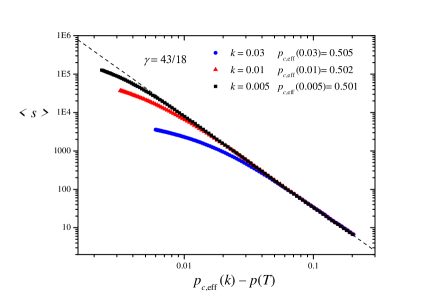
Figure 6: Average cluster size of the FPP balls calculated from Eq. (10) as a function of $p_{c,\text{eff}}(k)-p(T)$ for the three reference distributions. Corresponding $p_{c,\text{eff}}(k)$ are shown in the legend. Straight broken line corresponds to the theoretical scaling given in Eq. (9).

IV.3 Correlation length

Critical behavior in percolation theory is completely dominated by a single characteristic length, the correlation length $\xi$ Stauffer_03 , which stands for the crossover length scale below which the behavior is indistinguishable from that at $p_{c}$.

Given a single percolation cluster, its radius of gyration is defined by the average squared distance between two cluster sites:

$$R_{s}^{2}\equiv{1\over 2}\sum_{i,j}{|\textbf{r}_{i}-\textbf{r}_{j}|^{2}\over s^{2}},$$ (11)

where $\textbf{r}_{i}$ stands for the position vector of the $i$-th site of the cluster and the subscript $s$ stands for the cluster size. We can average this radius over all clusters of size $s$ to obtain $\overline{R_{s}^{2}}$. Finally, the average of $\overline{R_{s}^{2}}$ over all cluster sizes $s$ in the following way provides a standard definition of the squared correlation length Stauffer_03 :

$$\xi^{2}(p)\equiv 2{\sum_{s}\overline{R_{s}^{2}}s^{2}n_{s}(p)\over\sum_{s}s^{2}n_{s}(p)},$$ (12)

which is known to diverge as we approach the critical point ($p\rightarrow p_{c}$) as

$$\xi(p)\sim|p_{c}-p|^{-\nu},$$ (13)

with $\nu=4/3$ for $D=2$. Again, if we approach from above we have to exclude in the sum the contribution of the infinite cluster.

The correlation length is the radius of those clusters which mainly contribute to the second moment of the cluster size distribution. Near the percolation threshold this contribution comes from the clusters of size of the order of $s_{\xi}$ so we find

$$s_{\xi}\sim\xi^{D_{f}},$$ (14)

where $D_{f}$ is the fractal dimension of the infinite percolation cluster, $D_{f}=91/48$ for $D=2$.

If we turn now to our FPP problem and apply the equivalence discussed so far to Eq. (12), we deduce the following expression for the correlation length of the FPP balls:

$$\xi^{2}(p(T))=2{\sum_{s}\overline{R_{s}^{2}}\,sW_{s}(T)\over\sum_{s}sW_{s}(T)}.$$ (15)

Results regarding the correlation length have been displayed in Fig. 7 following the same scheme as in Fig. 6 for the average size. The similarity between both plots is not surprising since they correspond to moments of the same cluster size distribution. According to percolation theory, $s_{\xi}$ is exactly the cluster size that dominates the moments of the mass distribution, including the average cluster size $\langle s\rangle$ and the correlation length $\xi$. As a consequence, $\xi$ represents the radius of the clusters of size $s_{\xi}$. On the other hand, the radius $\xi_{o}$ of balls of size $s_{o}$ gives the crossover length scale below which the balls behave as percolation clusters. We can thus use here the explanation given for the average cluster size by considering the correlation length $\xi$ instead of $s_{\xi}$, and the cutoff radius $\xi_{o}$ instead of $s_{o}$. For probabilities such that $\xi(p)\ll\xi_{o}(p)$, the round-off effect is negligible since it only affects sizes much larger than the dominant size $s_{\xi}$. Thus, the correlation length of the FPP balls behaves as in the percolation problem. As we approach the critical point, $\xi$ diverges, becoming much larger than $\xi_{o}$. Due to the round-off effect size $s_{o}$ becomes the dominant term, yielding a deviation with respect to the scaling law. The crossover probability $p_{o}^{\star}$ is the same as for the average cluster size and is obtained when $\xi(p_{o}^{\star})$ is of the same order as $\xi_{o}(p_{o}^{\star})$.

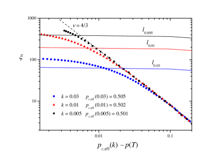
Figure 7: Correlation length of the FPP balls calculated from Eq. (15) as a function of $p_{c,\text{eff}}(k)-p(T)$ for the three reference distributions. Corresponding $p_{c,\text{eff}}(k)$ values are shown in the key. Straight broken line corresponds to the theoretical scaling given in Eq. (13). Continuous curves correspond to the length $\ell_{o}(T(p))$ obtained for each $k$ from the chain model presented in Sec. V.

IV.4 Percolation probability

The order parameter of the second-order phase transition observed in percolation is given by the percolation probability $\mathcal{P}$, or strength of the infinite cluster, defined as the probability that a randomly chosen site belongs to the infinite cluster. For $p\leq p_{c}$ we have $\mathcal{P}=0$, and it goes to zero as a power law as we approach the critical point from above ($p\rightarrow p_{c}^{+}$):

$$\mathcal{P}(p)\sim(p-p_{c})^{\beta},$$ (16)

where $\beta=5/36$ for $D=2$ is yet another critical exponent Stauffer_03 . Our purpose is to recover this exponent from the analysis of the FPP balls.

Let us define $G_{\textbf{x}}(T)$ as the probability that site $\mathbf{x}$ belongs to the FPP ball at passage time $T$,

$$G_{\textbf{x}}(T)=\text{Prob}\{\textbf{x}\in B(T)\}.$$ (17)

$G_{\textbf{x}}(T)$ is also the probability that the arrival time needed to reach site $\mathbf{x}$ is less than T, i.e. the cumulative distribution of the arrival time to node $\mathbf{x}$ at time $T$. Note that $G_{\textbf{x}}(T)$ is related to the probability density function $g_{\textbf{x}}(T)$ addressed in previous section and displayed in Fig. 3, through $g_{\textbf{x}}(T)=dG_{\textbf{x}}(T)/dT$. The behavior of $G_{\textbf{x}}(T)$ as a function of $p=F(T)$ for different sites along the axis for $k=0.005$ is shown in the top panel of Fig. 8.

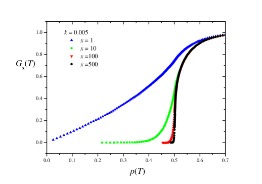
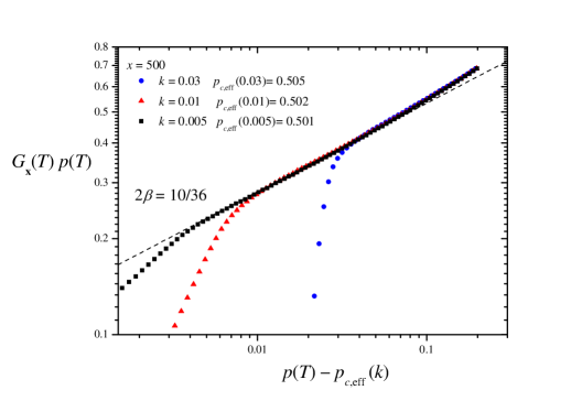
Figure 8: Strength of the infinite cluster. (Top) Probability that a node at position $x$ in the axis will belong to the ball with passage time $T$, as a function of $p=F(T)$ for $k=0.005$ and different distances: $x=1$, $10$, $100$ and $500$. (Bottom) $G_{\textbf{x}}(T)\,p(T)$ product as a function of $p(T)-p_{c,\text{eff}}(k)$ for a node at $x=500$ and the three reference distributions. The straight broken line represents the scaling behavior deduced in Eq. (18).

As we move away from the center node the curves become sharper around $p=1/2$ and, for large $x$, $G_{\textbf{x}}(T)$ tends to a limit function. That limit function is qualitatively very similar to the plot of the order parameter $\mathcal{P}$ as a function of $p$. For distant positions there is a minimum arrival time, which approaches very fast the critical passage time $T_{c}$ as $x\rightarrow\infty$. This result is consistent with the criticality of the percolation problem: at $p=p_{c}$ an infinite cluster that percolates through the lattice appears for the first time.

From these results and Eq. (17) we deduce that for $x\gg 1$, $G_{\textbf{x}}(T)$ is the probability that both the initial and the final points belong to the infinite cluster. In percolation theory this probability is given, for very long distances (and thus uncorrelated sites) by $\mathcal{P}^{2}$. Besides, this probability is conditioned on the known fact that the initial point (the center node) belongs to the cluster, so we have to divide the above expression by $p$. Our reasoning allow us to conjecture that for $x\gg 1$:

$$G_{\textbf{x}}(T)\approx{\mathcal{P}^{2}(p)\over p}\rightarrow{(p-p_{c})^{2\beta}\over p}\quad\mbox{as}\quad p\rightarrow p_{c},$$ (18)

using always $p=F(T)$. Numerical evidence for Eq. (18) is shown in the bottom panel of Fig. 8. The plot displays the values of the product $p\,G_{\textbf{x}}(T)$, obtained from the top panel of the figure, as a function of $p-p_{c,\text{eff}}(k)$, for the three levels of disorder. As in previous figures we obtain an excellent collapse of the curves into the expected power-law as $p\rightarrow p_{c,\text{eff}}(k)$, while deviations take place at the same crossover probabilities $p_{0}^{\star}$ obtained before for the mean cluster size and the correlation length.

IV.5 Fractal dimension of FPP balls

The infinite cluster at the critical point is a fractal, so its mass $M$ scales with the linear size $\ell$ as $M\sim\ell^{D_{f}}$, where $D_{f}$ is the fractal dimension ($D_{f}=91/48$ for $2D$). However, fractal behavior is also observed away from the critical point at length scales much smaller than the correlation length, so we have $M\sim\ell^{D_{f}}$ for $\ell\ll\xi$, and $M\sim\ell^{D^{\prime}}$ for $\ell\gg\xi$, with dimension $D^{\prime}$ depending on whether we are above or below the critical point (for $p>p_{c}$ we have $D^{\prime}=D$, the Euclidean dimension). Clusters look fractal on scales smaller than $\xi$ and this also applies to the relation between their mass $s$ and their linear size $R_{s}$: for $R_{s}\ll\xi$ or equivalently $s\ll s_{\xi}$ we find $s\sim R_{s}^{D_{f}}$, from which we can deduce Eq. (14).

In Fig. 9 we have shown the mass of FPP balls within circles of increasing radius $r$ centered at the origin, for extreme disorder $k=0.005$. To perform the analysis we have selected among all the FPP balls grown at critical passage time $T_{c}$ those with sizes contained in small intervals around three different sizes $s$. Results were averaged over all the balls within the same interval.

The plots show a constant slope which coincides with the fractal dimension for critical percolation (broken line). The final plateaux are not related to a crossover. They are due to the fact that clusters become finite with linear size $R_{s}$, so after $r\approx R_{s}$ the mass becomes constant. It is interesting to note that sizes $s=10^{5}$ and $s=10^{6}$ are larger than the corresponding cutoff size $s_{o}$ (above $10^{4}$, see Fig. 5), i.e. these clusters are influenced by the round-off. However, this effect does not seem to significantly change the internal structure of the balls, which is still fractal, so the main consequence of the round-off is the trimming of the branched edges.

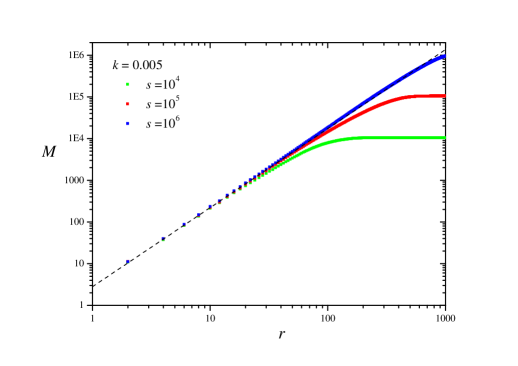
Figure 9: Mass of the FPP ball $B(T_{c})$ within a circle of radius $r$ centered at the origin for case $k=0.005$. Results correspond to the average over balls with sizes within the following intervals: (green) $s\in(1,1.1)\cdot 10^{4}$, (red) $s\in(1,1.1)\cdot 10^{5}$ and (blue) $s\in(1,1.1)\cdot 10^{6}$. The straight line corresponds with a power-law, $M\sim r^{91/48}$.

V Crossover length for percolation in the FPP model

Let us elaborate on the validity of the max principle that allows the mapping of the FPP into the percolation problem. Our purpose is to find an estimate for the cutoff values $\xi_{o}(p)$ and $s_{o}(p)$.

Another way to see the max principle is presented in the following experiment, which we call the chain model. Let us consider a linear array of $\ell$ sites and let us choose a time $T$. Then we fill the chain with $t$ values obtained by sampling the link-time distribution, but only keeping values which are smaller than $T$, i.e. if $t\geq T$ we disregard the value. These chains represent idealized versions of the minimal paths since they cannot include crossing-times larger than the passage time $T$. We define $\mathbf{P}$ as the probability for the sum of the link-times to be smaller than $T$:

$$\mathbf{P}_{o}(\ell,T)=\text{Prob}\left\{\sum_{i=1}^{\ell}t_{i}<T\;|\;t_{i}<T\right\}.$$ (19)

$\mathbf{P}_{o}(\ell,T)$ can be seen as the probability that the max principle holds at a length scale $\ell$ and passage time $T$. Our claim is the following: if there exists a cutoff length $\ell_{o}(T)$ such that

$$\mathbf{P}_{o}(\ell,T)\approx\begin{cases}1&\textrm{for }\ell\ll\ell_{o}(T),\\ \textrm{fast decay}&\textrm{for }\ell\gg\ell_{o}(T),\end{cases}$$ (20)

then $\xi_{o}(p)$ should behave as $\ell_{o}(T)$, always with $p=F(T)$. The numerical evidences that follow will support our claim.

Figure 10 shows two sets of results for $\mathbf{P}_{o}(\ell,T)$. In the top panel we display the dependence of $\mathbf{P}$ on $\ell$ for different arrival times $T$ (expressed as $p(T)$) and for fixed $k=0.005$. In the bottom panel the arrival time has been fixed to $T_{c}$ and the curves correspond to different strengths of the disorder (different values of $k$).

The first remarkable result is that $\mathbf{P}_{o}(\ell,T)$ shows an excellent agreement with the stretched exponential function:

$$\mathbf{P}_{o}(\ell,T)\approx\exp\left[-\left(\frac{\ell-1}{\ell_{o}(T)}\right)^{\phi_{o}(T)}\right].$$ (21)

The corresponding fits have been shown with colored continuous lines. As shown, the dependence of $\mathbf{P}$ on $\ell$ follows the behavior conjectured in Eq. (20) with $\ell_{o}(T)$ thus playing the role of a cutoff length. It is important to stress that we have obtained the same behaviour for the other link-time distributions investigated in this work (Log-Normal and Pareto).

We address now the behavior of the fitting parameters, the cutoff length $\ell_{o}(T)$ and the stretch exponent $\phi_{o}(T)$, displayed in the top and bottom panels of Fig. 11 respectively, as a function of the probability $p(T)$ for different values of $k$.

With regard to $\ell_{o}(T)$, our results support all the assumptions made in the previous section about $\xi_{o}$. For a given arrival time it increases monotonously with the disorder, and for a given disorder it is a continuously increasing function of the arrival time. We expect $\ell_{o}(T)$ to diverge for any arrival time as $o\rightarrow 0$. Interestingly, although $\ell_{o}(T)$ is not defined at $T=0$ it shows a well-defined positive limit. The same was found for the Log-Normal distribution while for Pareto the limit is $0$.

Another remarkable result is the change of behavior near the crossover point between weak and strong disorder ($k^{\star}=1.79$). For $k<k^{\star}$ we obtain $\ell_{o}(T)>1$ for all $T$, in consistency with our assumption that under strong disorder conditions there is always a length scale below which the FPP model behaves as a percolation lattice. However, if $k>k^{\star}$ (see e.g. case $k=3$) the fitted values of $\ell_{o}(T)$ are smaller than 1 for $p<1$. Indeed, as $k$ increases above $k^{\star}$ the decay of $\mathbf{P}_{o}(\ell,T)$ after $\ell=1$ becomes sharper and the expression given in Eq. (20) approaches the step function: $\mathbf{P}_{o}(\ell,T)=1$ if $\ell=1$ and $\mathbf{P}_{o}(\ell,T)=0$ if $\ell>1$. As a consequence, the fitted values of $\ell_{o}(T)$ approach $0$ as $k$ increases for finite $T$ (or $p<1$). We can then expect that the function $\ell_{o}(p)-1$ approaches the delta function $\delta(1-p)$ as $k\rightarrow\infty$. We will return to this issue when we address the homogeneous case. Nevertheless, the change of behavior of $\ell_{o}(T)$ near the crossover point $o^{\star}$ points to it as a reliable estimate for the crossover length $\xi_{o}$.

With regard to the stretch exponent $\phi_{o}(T)$, displayed in the bottom panel of Fig. 11, we observe that for a given $p$ it increases with disorder and seems to approach a constant value above $1.7$ under strong disorder conditions. We also notice that, in this regime, it roughly remains constant with $p$. Only for large $k$ we observe a smooth increase with passage time that sharpens as we approach $p=1$.

In order to check the relation between the cutoff length $\ell_{o}$ obtained from our chain model and the crossover length $\xi_{o}$ postulated as the length scale under which the FPP model behaves as a percolation lattice, we have represented the corresponding curves of $\ell_{o}$ in the plot of the correlation length $\xi$ of the FPP balls, Fig. 7. The comparison between both magnitudes provide numerical evidence of our claims. For probabilities $p$ such as $\xi\ll\ell_{o}$, the correlation length of the balls follows the scaling behavior predicted from percolation theory. As $p$ increases and $\xi$ approaches $\ell_{o}$, the effect of the round-off makes $\xi$ depart from the percolation prediction. As discussed, this deviation takes place at $p_{o}^{\star}$, where both quantities become of the same order. A crossover towards a new behavior that its controlled by $\ell_{o}$ takes place, in which we expect that $\xi$ will grow as $\ell_{o}$ for $p\gg p_{o}^{\star}$.

We can provide further numerical evidence of the reliability of $\ell_{o}$ as an estimator for the crossover length $\xi_{o}$. For example, following our reasoning we can conjecture that $\ell_{o}$ is the radius of the balls with cutoff-size $s_{o}$, so we can expect:

$$s_{o}\sim\ell_{o}^{D}.$$ (22)

Then, according to Eq. (7) the number of clusters of size $s_{o}$, $n_{s_{o}}$, must behave as:

$$n_{s_{o}}\sim s_{o}^{-\tau}\sim\ell_{o}^{-\tau D}.$$ (23)

For probabilities close to the percolation threshold so that $s_{o}\ll s_{\xi}$, the size distributions obtained from different $k$ should collapse into a single universal curve if we rescale the size $s$ by $s_{o}$, and $n_{s}$ by $n_{s_{o}}$. The rescaling of the distributions displayed in Fig. 5 has been shown in Fig. 12, and a quite satisfactory collapse of the three distributions is obtained.

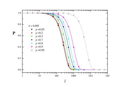
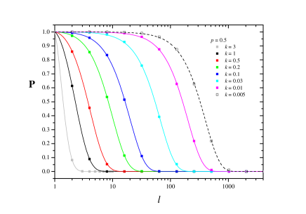
Figure 10: Probability $\mathbf{P}$ calculated from Eq. (19) over an ensemble of $10^{6}$ chains as a function of the chain length $\ell$ for: (top) $k=0.005$ and different passage times represented by $p(T)$; (bottom) $p=0.5$ and different $k$. Points correspond to results from simulations while continuous lines represent the corresponding fits to function in Eq. (21).

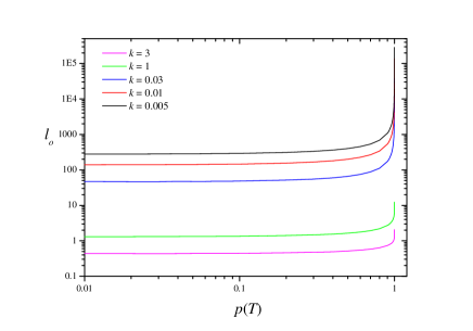
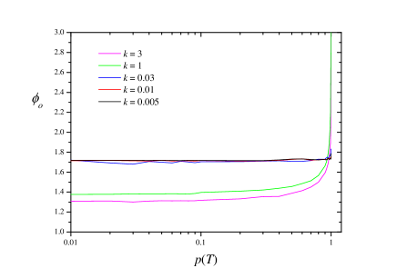
Figure 11: Fitted values of the cutoff length $\ell_{o}(T)$ (top) and the stretch exponent $\phi_{o}(T)$ (bottom) as a function of probability for different strengths of disorder, $p(T)$.

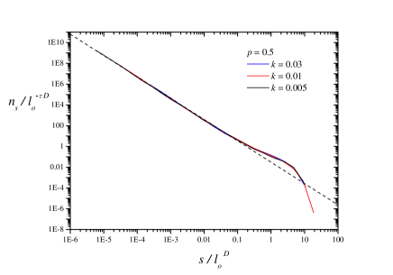
Figure 12: Rescaling of the size distributions displayed in Fig. 5. For each curve, ball size $s$ has been rescaled by $\ell_{o}^{D}$ ($D=2$) with values: $\ell_{0.03}(p=0.5)=65.83$, $\ell_{0.01}(p=0.5)=199.34$ and $\ell_{0.005}(p=0.5)=399.72$, obtained from the simulations of the chain model. $n_{s}$ has been rescaled by $\ell_{o}^{-\tau D}$ according to Eq. (23).

VI Discussion: crossover between percolation and KPZ scaling

VI.1 Strong disorder regime $o\ll o^{\star}$

The growth of FPP balls is controlled by two characteristic lengths: the crossover length $\xi_{o}$ which determines the length scale below which the FPP model is essentially a bond-percolation lattice with $p=F(T)$, and the correlation length $\xi$ intrinsic to the percolation problem. Whereas the behavior of $\xi$ is well-known from percolation theory –at least close to the critical point–, we can assume that the crossover length $\xi_{o}$ is related to the cutoff length $\ell_{o}$ of the chain model. This is a strong assumption because the link-times traversed by actual geodesics are correlated to each other by means of the minimal time principle, in contrast to the uncorrelated link-times assumed in our model.

For some distributions such as Weibull or Log-Normal, $\ell_{o}(T)$ has a well-defined positive limit when $T\rightarrow 0$, so we can expect the same for $\xi_{o}$. Since $\xi$ is initially $0$, we conclude that FPP balls will display initial percolation-like growth provided this limit value is larger than 1. This seems to be guaranteed in the strong disorder regime $o<o^{\star}$. For the Pareto distribution we find $\ell_{o}(T)\rightarrow 0$ as $T\rightarrow 0$. However, the increase of $\ell_{o}(T)$ with passage time $T$ is faster than the increase of $\xi(p)$ with probability $p(T)$, hence allowing an initial percolation phase also in this case.

Percolation-like growth will take place whenever $\xi$ is much smaller than $\xi_{o}$. In this regime, the growth of FPP balls as the arrival time $T$ increases can be mapped into the growth of the percolation clusters at increasing occupation probability $p=F(T)$. That regime continues until $\xi$ becomes of the same order as $\xi_{o}$, which takes place at a certain arrival time $T_{o}^{\star}$. This crossover time is upper bounded by the critical passage time, i.e. $T_{o}^{\star}<T_{c}$, because $\xi$ diverges at the critical point. Under extreme disorder conditions, i.e. for small but positive values of the order parameter $o$, $\xi_{o}$ is large, $T_{o}^{\star}$ is close to $T_{c}$, and we can observe the fractal clusters obtained in percolation. We expect that $T_{o}^{\star}\rightarrow T_{c}$ as $o\rightarrow 0$, i.e. for infinite disorder.

Once the crossover arrival time $T_{o}^{\star}$ has been reached, we enter into a transient regime that evolves towards KPZ scaling. Two different types of growth at two different length scales take place simultaneously. At scales below $\xi_{o}$, percolation-like growth still continues with a percolation correlation length $\xi$ that rapidly decreases with time above $T_{c}$ ($p>p_{c}$). The increase of $p$ fills the inner holes and cavities, and smoothes the irregularities of the outer perimeter. Above $T_{c}$, the cutoff length $\xi_{o}$ prevents the incipient infinite percolation cluster from spreading along the lattice. At larger scales the growth of the ball is controlled by the growth of $\xi_{o}$, which simply reflects the fact that minimal paths are limited by their length. FPP balls becomes compact with a regular shape, a process that finally leads to KPZ scaling.

This transient regime would last until the effects of percolation vanish, i.e. when $p=1$, which corresponds to an infinite arrival time. We can make, however, some speculations. For example, in Fig. 4 we showed the fluctuations of the arrival time to points along the axis for different levels of disorder. Now we know that $k=0.5$, $0.3$ or $0.2$ are not small enough to display the criticality of percolation, but the disorder is in fact strong enough to reveal percolation effects in the behavior of the arrival-time fluctuations. In each curve of the figure with $k<k^{\star}$ we have marked three representative lengths obtained from the chain model. As an approximation of $\xi_{o}$ we have considered $\ell_{o}(T_{c})$, indicated with the vertical segments. In order to estimate the range of the percolation effects and, thus, the crossover towards KPZ scaling, we have represented in each curve with a grey rectangle the interval $(\ell_{o}(T(p=0.99)),\ell_{o}(T(p=0.999))$. Despite the approximations and the simplicity of our model, the crossover points are in a reasonably good agreement with the behavior displayed by the fluctuations.

Both the crossover length $\xi_{o}$ and the associated cutoff size $s_{o}$ increase with disorder and we expect them to diverge as $o\rightarrow 0$. The kinetics of the approach towards “infinite” disorder depends on the specific distribution. For example, for the Weibull distribution we obtain the following limit of Eq. (5), valid for $p\in[0,1)$:

$$\lim_{k\rightarrow 0}T(p)=\begin{cases}0&\mbox{if }\;p<p_{0}\\ \lambda&\mbox{if }\;p=p_{0}\\ \infty&\mbox{if }\;p>p_{0}\end{cases}$$ (24)

where $p_{0}=1-e^{-1}=0.63$. After an infinitesimal arrival time the balls take the form of the percolation clusters obtained at $p=p_{0}$. This is followed by an infinitely slow growth. At the limit we have $B(T)=B(0)$ for $T>0$, where $B(0)$ is the percolation cluster obtained at $p=p_{0}$.

For the Log-Normal distribution we have:

$$T(p)=e^{\mu}\exp{\left(\sqrt{2\sigma^{2}}\mbox{erf}^{-1}\left[2p-1\right]\right)},$$ (25)

where $\mbox{erf}^{-1}(x)$ is the inverse error function, and the approach to the critical point is similar:

$$\lim_{\sigma\rightarrow\infty}T(p)=\begin{cases}0&\mbox{if }\;p<p_{0}\\ e^{\mu}&\mbox{if }\;p=p_{0}\\ \infty&\mbox{if }\;p>p_{0}\end{cases}$$ (26)

but now we have $p_{0}=1/2$, i.e. the critical ball is just the critical percolation cluster obtained at the critical probability.

Finally, for the Pareto distribution we have

$$T(p)=t_{m}\left(\frac{1}{1-p}\right)^{1/\alpha},$$ (27)

and we obtain:

$$\lim_{\alpha\rightarrow 0}T(p)=\infty\quad\mbox{for }\;0<p<1,$$ (28)

which means that we must resort to increasingly large arrival times in order to observe the growth.

VI.2 Weak disorder regime $o\gg o^{\star}$

It is interesting to finish this work by considering the homogeneous case in which all links have the same crossing time $\tau_{0}$. As discussed in Sec. II and shown in Appendix A, this case corresponds to the limit $o\rightarrow\infty$ of the link-time distributions, even though the specific value of $\tau_{0}$ depends on the distribution function (see Eq. (35)): $\tau_{0}=\lambda,e^{\mu},t_{m}$ for Weibull, Log-Normal and Pareto respectively.

For the homogeneous case the chain model gives exactly $\ell_{o}(T)=T/\tau_{0}$. Now we can use the following result, which applies to all distributions:

$$\lim_{o\rightarrow\infty}{T(p)}=\tau_{0}\quad\mbox{for }p<1,$$ (29)

to obtain

$$\lim_{o\rightarrow\infty}\ell_{o}(p)=1\quad\mbox{for }p<1.$$ (30)

It is important to note that this limit strictly holds for probabilities smaller than 1. At the limit $p\rightarrow 1$ we obtain $\ell_{o}\rightarrow\infty$.

This result confirms the assumption made in the previous section:

$$\lim_{o\rightarrow\infty}\ell_{o}(p)-1=\delta(1-p),$$ (31)

and also shows that for a weak enough disorder we cannot observe the percolation phase because it only extends to a few sites.

As a numerical example, let us consider the distribution Wei$(1,3)$ where value $k=3$ is above the crossover value $k^{\star}\approx 1.79$. From the chain model we obtain $\ell_{3}(p=0.99999)\approx 1.86$, which roughly means that percolation effects up to a probability of $p=0.99999$ are limited to a length scale of less than two lattice units. On the other hand, the arrival time corresponding to that probability is $T(p=0.99999)\approx 2.26$. Now we can use the value of the mean time for that distribution, $\tau\approx 0.89$ (close to $\tau_{0}=\lambda=1$), to obtain $T/\tau\approx 2.53$, which provides a good estimate of $\ell_{3}(p=0.99999)$. This result shows that we cannot observe percolation effects even at disorders close to the crossover value $o^{\star}$.

VII Conclusions and further work

In this work we have characterized the dynamics of first-passage percolation (FPP) square lattices under extreme disorder, as opposed to the weak-disorder regime, which is dominated by KPZ universality. Several link-time distributions were considered which allows for a continuous variation of the disorder strength through the so-called order parameter $o$. A crossover value $o^{\star}$ (for which $d_{c}=1$) was proposed as the crossover point between the two regimes.

Our study has revealed that, given a certain level of disorder, there exists a characteristic length scale $\xi_{o}$ below which the FPP model behaves essentially as a bond-percolation lattice. Arrival times at length scales smaller that $\xi_{o}$ follow a max principle which allow us to establish a continuous mapping of FPP passage time $T$ into the probability $p$ of a bond being open in bond-percolation. The basic assumption is that the sum of link-times along the geodesic can be approximated by their maximum value. As a result the mapping has the form $p=F(T)$, where $F$ denotes the cumulative distribution function for the link-times.

At length scales below $\xi_{o}$ the FPP model displays the same criticality found in the second-order phase transition observed in bond-percolation. The average value of the arrival time to different sites becomes ill-defined and the geodesic between neighboring points of the lattice can become arbitrarily large, instead of using a single link as in the weak-disorder regime. Through a comprehensive scaling analysis of the FPP balls we have been able to observe the critical exponents characterizing the scaling of the percolation clusters near the critical point, including their fractal structure, instead of the reasonably rough circular balls within the KPZ universality class.

The dynamics of the FPP growth under strong disorder conditions is the result of the interplay between this crossover length $\xi_{o}$ and the correlation length $\xi$ characteristic of bond-percolation, both evolving dynamically with passage time $T$. When $\xi\ll\xi_{0}$ the growth of the FPP balls with passage time $T$ can be mapped into the growth of the percolation clusters with increasing probability $p=F(t)$, which resembles a sort of invasion percolation. At a certain passage time $T_{o}^{\star}$ (which is upper bounded by the critical arrival time $T_{c}$), $\xi$ becomes of the same order of $\xi_{0}$. Further growth leads to the failure of the maximality assumption: the sum of the link-times along a geodesic may become significantly different from the maximal value found along it. Thus balls must start a rounding-off process that yields a crossover towards KPZ-scaling. Therefore, for long enough distances we always recover the KPZ regime.

The crossover length $\xi_{o}$ (as well as other related magnitudes defined as a function of the order parameter) increases as the disorder becomes stronger and seems to diverge when the order parameter approaches zero, which we call the infinite disorder limit. The infinite disorder limit of these models presents very intriguing features, which might be related to critical or supercritical FPP cases, that we intend to ascertain in future work. We have provided very preliminary evidences pointing to that idea. Note, for example, that limit when $o\rightarrow 0$ of the Weibull and Log-Normal distribution functions given in Eqs. (32) and (33) are, for non-zero $t$, $F(t)=1-e^{-1}=0.63$ and $F(t)=1/2$ respectively. They have the form of the Bernoulli distribution (except for $t=0$) in which link-times can be zero (open bonds) with probability $p_{0}$ and infinite (closed bonds) with probability $1-p_{0}$, with $p_{0}$ given by the above values. For the Weibull distribution we have $p_{0}>p_{c}$ and its infinite-disorder limit might be related to critical FPP, whereas for the Log-Normal we have $p_{0}=p_{c}$ and thus the supercritical case. Since length $\xi_{o}$ determines the crossover length scale between percolation and KPZ phases, and it diverges at the infinite-disorder limit, certainly it would be very interesting to study the criticality near this limit.

Another direction of future work is to elaborate more on the estimate for $\xi_{o}$ derived from the chain model. Although the numerical evidences presented here support its validity, there are still many open questions that deserve additional work, including a theoretical justification of Eq. (21) and the generalization of the observed behaviors to other link-time distributions.

Appendix A Link-time distributions

The analysis performed in this work requires link-time distributions with the following properties: (a) the link-times must be always positive; (b) the range of disorder must be large, i.e. for some range of the distribution parameters, the deviation must be larger than the average value. We have chosen three distributions fulfilling those requirements: Weibull, Log-Normal and Pareto. They have been chosen for several reasons. First, their mathematical expressions allow a simple analytic treatment. Also, we can easily tune the strength of the disorder through a single parameter, the shape parameter. Besides, some of them (e.g. Weibull) generalizes a number of other distributions. The mathematical expressions for the probability density function $f(t)$ and the cumulative distribution function $F(t)$ of those distributions are:

1. The Weibull distribution, Wei$(\lambda,k)$:

   $$f(t) ={k\over\lambda}\left({t\over\lambda}\right)^{k-1}\exp\left(-(t/\lambda)^{k}\right),$$ (32)

   $$F(t) =1-\exp\left(-(t/\lambda)^{k}\right).$$

   The results displayed in this work do not depend on the scale parameter $\lambda$, so we have considered $\lambda=1$ in all the numerical simulations. As we will see, it is the shape parameter $k$ which completely determines the strength of the disorder.

2. The Log-Normal distribution, LogN$(\mu,\sigma)$:

   $$f(t) ={1\over t\sqrt{2\pi\sigma^{2}}}\exp{\left[-{(\ln t-\mu)^{2}\over 2\sigma^{2}}\right]},$$ (33)

   $$F(t) =\frac{1}{2}+\frac{1}{2}\mbox{erf}\left[\frac{\ln t-\mu}{\sqrt{2\sigma^{2}}}\right].$$

   The above comment about the parameters of the Weibull distribution also applies here to parameters $\mu$ and $\sigma$ respectively.

3. The Pareto distribution, Par$(t_{m},\alpha)$:

   $$f(t) =\begin{cases}{\alpha t_{m}^{\alpha}\over t^{\alpha+1}}&\mbox{if }\;t\geq t_{m}\\ 0&\mbox{if }\;t<t_{m}\end{cases}$$ (34)

   $$F(t) =\begin{cases}1-\left({t_{m}\over t}\right)^{\alpha}&\mbox{if }\;t\geq t_{m}\\ 0&\mbox{if }\;t<t_{m}\end{cases}$$

   with the above remark applying to scale $t_{m}$ and shape $\alpha$ parameters respectively.

The homogeneous case discussed in Sec. II is obtained at the following limits of the above distributions:

$$\lim_{k\rightarrow\infty}\mbox{Wei}(\lambda,k) =\delta(t-\lambda),$$ (35)

$$\lim_{\sigma\rightarrow 0}\mbox{LogN}(\mu,\sigma) =\delta(t-e^{\mu}),$$

$$\lim_{\alpha\rightarrow\infty}\mbox{Par}(t_{m},\alpha) =\delta(t-t_{m}).$$

A relevant parameter in our discussion is $d_{c}=(1/3)(\tau/s)^{2}$, where $\tau$ is the mean value and $s$ the standard deviation of the distributions (when they exist). For the Weibull distribution we find:

$$d_{c}(k)={1\over 3}\frac{\Gamma^{2}\left[1+{1\over k}\right]}{\Gamma\left[1+{2\over k}\right]-\Gamma^{2}\left[1+{1\over k}\right]},$$ (36)

and the crossover value of $k$ for which $d_{c}=1$, denoted here as $k^{\star}$, is

$$k^{\star}\equiv k(d_{c}=1)\approx 1.79.$$ (37)

For the Log-Normal distribution we have:

$$d_{c}(\sigma)={1\over 3}\frac{1}{e^{\sigma^{2}}-1}\quad\mbox{with}\quad\sigma^{\star}\approx 0.54,$$ (38)

and for Pareto:

$$d_{c}(\alpha)={1\over 3}\alpha(\alpha-2)\quad\mbox{with}\quad\alpha^{\star}=3.$$ (39)

Note that the last expression only holds for $\alpha>2$ since the standard deviation $s$ diverges when $\alpha\leq 2$ and the mean time $\tau$ diverges if $\alpha\leq 1$. For $\alpha\leq 2$ we shall assume that $d_{c}=0$.

In the three cases $d_{c}$ is a monotonic function of the shape parameter: it decreases and approaches $0$ as the dispersion of the distribution increases ($k\rightarrow 0$, $\sigma\rightarrow\infty$ and $\alpha\rightarrow 0$), and diverges as the distributions approach the delta distribution ($k\rightarrow\infty$, $\sigma\rightarrow 0$ and $\alpha\rightarrow\infty$).

References

- (1) D. Nelson, T. Piran and S. Weinberg, Statistical Mechanics of Membranes and Surfaces, World Scientific, Singapore (2004).
- (2) D. H. Boal, Mechanics of the cell, Cambridge University Press, Cambridge (2012).
- (3) C. Itzykson and J.-M. Drouffe, Statistical Field Theory, Cambridge University Press, Cambridge (1991).
- (4) B. Booß-Bavnbek, G. Esposito and M. Lesch, New paths towards quantum gravity, Springer, Berlin (2009).
- (5) J. Ambjørn, B. Durhuus and T. Jonsson, Quantum Geometry: A Statistical Field Theory Approach, Cambridge University Press, Cambridge (1997).
- (6) S.N. Santalla, J. Rodriguez-Laguna, T. LaGatta and R. Cuerno, Random geometry and the Kardar–Parisi–Zhang universality class, New J. Phys. 17 033018 (2015).
- (7) S.N. Santalla, J. Rodriguez-Laguna, A. Celi and R. Cuerno, Topology and the Kardar–Parisi–Zhang universality class, J. Stat. Mech. 023201 (2017).
- (8) M. Kardar, G. Parisi and Y.-C. Zhang, Dynamic Scaling of Growing Interfaces, Phys. Rev. Lett. 56, 889 (1986).
- (9) A.-L. Barabási and H. E. Stanley, Fractal Concepts in Surface Growth, Cambridge University Press, Cambridge (1995).
- (10) J. Krug, Origins of scale invariance in growth processes, Adv. Phys. 46, 139 (1997).
- (11) T. Kriecherbauer and J. Krug, A pedestrian’s view on interacting particle systems, KPZ universality and random matrices, J. Phys. A: Math. Theor. 43, 403001 (2010).
- (12) T. Halpin-Healy and K. Takeuchi, A KPZ Cocktail- Shaken, not stirred: Toasting 30 years of kinetically roughened surfaces, J. Stat. Phys. 160, 794 (2015).
- (13) M. Prähofer and H. Spohn, Scale invariance of the PNG droplet and the Airy process, J. Stat. Phys. 108, 1071 (2002).
- (14) K. A. Takeuchi, M. Sano, T. Sasamoto and H. Spohn, Growing interfaces uncover universal fluctuations behind scale invariance, Sci. Rep. 1, 34 (2011).
- (15) I. Corwin, J. Quastel and D. Ramenik, Continuum statistics of the Airy2 process, Comm. Math. Phys. 317, 347 (2013).
- (16) J. M. Hammersley and D. J. A. Welsh, “First-passage percolation, subadditive processes, stochastic networks and generalized renewal theory”, in Bernoulli, Bayes, Laplace anniversary volume, J. Neyman and L. M. LeCam eds., Springer-Verlag (1965), p. 61.
- (17) C. D. Howard, “Models of first passage percolation”, in Probability on discrete structures, H. Kesten ed., Springer, Berlin (2004), p. 125–173.
- (18) A. Auffinger, M. Damron and J. Hanson, 50 years of FPP, University Lecture Series 68, American Mathematical Society (2017).
- (19) M. Kardar and Y.-C. Zhang, Scaling of Directed Polymers in Random Media, Phys. Rev. Lett. 58, 2087 (1987).
- (20) J. Krug and H. Spohn, “Kinetic roughening of growing surfaces”, in Solids far from equilibrium, C. Godrèche ed., Cambridge University Press, Cambridge (1991).
- (21) T. Halpin-Healy and Y.-C. Zhang, Kinetic roughening phenomena, stochastic growth, directed polymers and all that. Aspects of multidisciplinary statistical mechanics, Phys. Rep. 254, 215 (1995).
- (22) D.B. Abraham, L. Fontes, C.W. Newman and M.S.T. Piza, Surface deconstruction and roughening in the multiziggurat model of wetting, Phys. Rev. E 52, R1257 (1995).
- (23) S. Beyme and C. Leung, A stochastic process model of the hop count distribution in wireless sensor networks, Ad Hoc Netw. 17, 60 (2014).
- (24) G. Kordzakhia and S.P. Lalley, A two-species competition model on , Stoch. Proc. App. 115, 781 (2005).
- (25) R. Bundschuh and T. Hwa, An analytic study of the phase transition line in local sequence alignment with gaps, Discr. Appl. Math. 104, 113 (2000).
- (26) S. Chatterjee, 32.The universal relation between scaling exponents in first-passage percolation, Ann. Math. 177, 663 (2013).
- (27) H. Kesten, Percolation theory and first-passage percolation, Ann. Prob. 15, 1231 (1987).
- (28) P. Córdoba-Torres, S.N. Santalla, R. Cuerno and J. Rodríguez-Laguna, Kardar-Parisi-Zhang universality in first passage percolation: the role of geodesic degeneracy, J. Stat. Mech. 063212 (2018).
- (29) D. Stauffer and A. Aharony, An introduction to percolation theory, second edition, Taylor & Francis (2003).
- (30) M. Damron, W.-K. Lam and X. Wang, Asymptotics for 2D critical first passage percolation, Ann. Prob. 45, 2941 (2017).
- (31) M. Damron, J. Hanson and W.-K. Lam, Universality of the time constant for 2D critical first-passage percolation, arXiv:1904.12009 [math.PR] (2019).
- (32) C.-L. Yao, Law of large numbers for critical first-passage percolation on the triangular lattice, Electron. Commun. Probab. 19, 1 (2014).
- (33) C.-L. Yao, Limit theorems for critical first-passage percolation on the triangular lattice, Stoch. Proc. App. 128, 445 (2018).
- (34) H. Kesten and Y. Zhang, A central limit theorem for “critical” first-passage percolation in two-dimensions, Probab. Theory Rel. 107, 137 (1997).
- (35) Y. Zhang, Supercritical behaviors in first-passage percolation, Stoch. Proc. App. 59, 251 (1995).
- (36) O. Garet and R. Marchand, Large deviations for the chemical distance in supercritical Bernoulli percolation, Ann. Prob. 35, 833 (2007).
- (37) C. Yao, A note on geodesics for supercritical continuum percolation, Stat. Prob. Lett. 83, 797 (2013).
- (38) M. Aizenman, H. Kesten and C. Newman, Uniqueness of the infinite cluster and continuity of connectivity functions for short and long range percolation, Comm. Math. Phys. 111, 503 (1987).
- (39) H. Kesten, “Aspects of first-passage percolation”, in Lecture Notes in Mathematics 1180, Springer, Berlin (1986).
- (40) J.T. Chayes adn L. Chayes, “Percolation and random media”, in Critica Phenomena, Random Systems and Gauge Theories, Les Houches Session XLIII 1984, K. Osterwalder and R. Stora eds., 1000-1142, North-Holland, Amsterdam (1986).
- (41) R.T. Smythe and J.C. Wierman, “First-Passage Percolation on the Square Lattice”, in Lecture Notes in Mathematics 671, Springer, New York (1978).
- (42) A. P. Kartun-Giles, M. Barthelemy and C. P. Dettmann, Shape of shortest paths in random spatial networks, Phys. Rev. E 100, 032315 (2019).
- (43) A.L. Ritzenberg and R.J. Cohen, First passage percolation: scaling and critical exponents, Phys. Rev. B 30, 4038 (1984).
- (44) A.R. Kerstein, Contact propagation: percolation and other scaling regimes, Phys. Rev. B 31, 321 (1985).
- (45) A.R. Kerstein, Scaling law for the contact-propagation regime of first-passage percolation, Phys. Rev. B 31, 7472 (1985).
- (46) A.R. Kerstein and B.F. Edwards, Crossover from contact propagation to chemical propagation in first-passage percolation, Phys. Rev. B 33, 3353 (1986).
- (47) O. Garet and R. Marchand, Moderate deviations for the chemical distance in Bernoulli percolation, ALEA Lat. Am. J. Probab. Math. Stat. 7, 171 (2010).
- (48) N. Posé, K.J. Schrenk, N.A.M. Araújo and H.J. Herrmann, Shortest path and Schramm-Loewner evolution, Sci. Rep. 4, 5495 (2014).
- (49) P. Di Francesco, P. Matthieu and D. Sénéchal, Conformal Field Theory, Springer, Berlin (1997).