Learning from Discriminatory Training Data

Abstract.

Supervised learning systems are trained using historical data and, if the data was tainted by discrimination, they may unintentionally learn to discriminate against protected groups. We propose that fair learning methods, despite training on potentially discriminatory datasets, shall perform well on fair test datasets. Such dataset shifts crystallize application scenarios for specific fair learning methods. For instance, the removal of direct discrimination can be represented as a particular dataset shift problem. For this scenario, we propose a learning method that provably minimizes model error on fair datasets, while blindly training on datasets poisoned with direct additive discrimination. The method is compatible with existing legal systems and provides a solution to the widely discussed issue of protected groups’ intersectionality by striking a balance between the protected groups. Technically, the method applies probabilistic interventions, has causal and counterfactual formulations, and is computationally lightweight — it can be used with any supervised learning model to prevent discrimination via proxies while maximizing model accuracy for business necessity.

1. Introduction

With the growth of algorithmic decision-making systems in highly consequential domains such as finance and criminal justice, lawmakers have refocused their broader equity agendas to now include assurances that such algorithms do not discriminate. That is, algorithmic decision-making systems shall not treat someone unfavorably because of their membership to a particular group, characterized by a protected attribute such as race or gender. With this shifted focus, lawmakers in recent years have increasingly proposed new guidelines and orders that aim to prevent algorithmic discrimination, e.g., the U.S. blueprint for an “A.I. Bill of Rights” in 2022 (Blueprint for an AI Bill of Rights, 2022). These proposals are typically based on legal (Title VII of the Civil Rights Act, 1964; The Fair Housing Act, 1968) and social science (Ture et al., 1968; Altman, 2016; Lippert-Rasmussen, 2012) contexts, where the key basis for identifying algorithmic discrimination is whether there is a disparate treatment or unjustified disparate impact on the members of some protected group. To prevent disparate treatment, the law often forbids the use of certain protected attributes, $Z$, such as race or gender, in decision-making, e.g., in hiring. Thus, these decisions, $Y$, shall be based on a set of relevant attributes, $\bm{X}$, and should not depend on the protected attribute, $Z$, i.e., $\operatorname*{\textit{P}}(y|\bm{x},z)=\operatorname*{\textit{P}}(y|\bm{x},z^{\prime})$ for any $z,z^{\prime}$, ensuring that there is no disparate treatment. We refer to this kind of discrimination as direct discrimination (or lack of thereof), because of the direct use of the protected attribute $Z$.

Figure 1. Training data can be tainted in two ways: individuals belonging to underprivileged groups may be undersampled and, hence, models trained on this data may make larger errors for these groups (B), some of the labels in the training data may be incorrect due to historic discrimination and, hence, models trained on this data may be biased against the underprivileged groups (C). These two dataset issues represent a covariate shift and concept shift, respectively. This paper addresses discriminatory concept shifts.

Despite the introduction of laws prohibiting direct discrimination in the 20th century, such protections were sometimes circumvented by the use of attributes correlated with the protected attribute as proxies. One example of this is the practice of “redlining” done by U.S. financial institutions. That is, these institutions systematically denied loans and services to customers based on if they resided in neighborhoods with populations largely comprised of racial and ethnic minorities (Zenou and Boccard, 2000; Hernandez, 2009). In order to prevent such inducement of discrimination via proxy attributes, legal systems have established that the impact of a decision-making process should be the same across groups differing in protected attributes (Lippert-Rasmussen, 2012; Altman, 2016; Title VII of the Civil Rights Act, 1964; The Fair Housing Act, 1968), i.e., $\operatorname*{\textit{P}}(y|z_{1})=\operatorname*{\textit{P}}(y|z_{2})$. Such protections are also legally necessary for decision-making systems (on Further Advancing Racial Equity and for Underserved Communities Through The Federal Government, 2023), especially since data-rich machine learning systems can often find accurate surrogates for protected attributes when a large enough set of legitimate-looking variables is available, resulting in discrimination via association (Wachter, 2019). As a defense for allowing disparate impact across groups, these laws often have provisions allowing for such disparity if there is a “justified reason” or “business necessity clause” (Title VII of the Civil Rights Act, 1964). For instance, in the 1970s it was found that females were less often admitted than males in graduate admissions to University of California Berkeley (Bickel et al., 1975). However, females applied to departments with lower admission rates than males and the overall admissions process was judged legal. The provisions allowing for disparate impact, however, conflict with the statistical notions of fairness, the fairness definitions most common in algorithmic fairness literature (Lipton and Steinhardt, 2019). These notions typically call for parity of a statistical measure, e.g., impact parity: $\operatorname*{\textit{P}}(y|z_{1})=\operatorname*{\textit{P}}(y|z_{2})$ (Barocas et al., 2019), which prevents the usage of attributes related to the protected-attribute. To address the challenges with business necessity and proxies, and to develop a method that is transparent and communicable to lawmakers and courtroom officials, we employed explainability measures to remove direct discrimination without the inducement of discrimination (Grabowicz et al., 2022). Our prior work, however, did not discuss the real-world setting of multiple protected attributes, did not specify the training dataset issues, and was not optimally accurate — we address these gaps in this study.

In legal texts, the prevention of discrimination spans across many groups defined over multiple protected attributes, e.g, race, gender, and religion (Blueprint for an AI Bill of Rights, 2022; Title VII of the Civil Rights Act, 1964; The Fair Housing Act, 1968). Despite this, there rarely exists any legal mechanisms accounting for discrimination based on the intersection of the protected attributes an individual may have – a concept known as “intersectionality” which has been famously spotlighted by social experts in recent decades (Crenshaw, 2017). The need for such mechanisms can be seen in criminal justice settings such as COMPAS (Larson et al., 2016), where it is well documented that certain intersections of age, race, and sex experience more discriminatory outcomes, e.g, young Black males (Rovner, 2018). With the lack of legal support on preventing discrimination on these intersections, it is unsurprising that many fair learning methods do not operate in such settings and even fewer report results in it (Wang et al., 2022). In this work, we address this setting. Doing so is crucial for algorithmic fairness, as prior studies have shown that learning methods can be fair with respect to protected attributes separately, such as race and sex, while being discriminatory to intersections of attributes, e.g., Black females or Black males (Kearns et al., 2018).

Another crucial challenge is how to clarify application scenarios of algorithmic fairness methods. With this clarification, policymakers could utilize the information about such scenarios to shape future legislature regulating consequential algorithmic decision-making. Therefore, we propose to distinguish between various data issues and tie them with the methods that address these issues. This task, however, has received much less research attention than the fair learning methods themselves. Unfortunately, the research community that studies the data issues for supervised learning, so-called dataset shifts (Widmer and Kubat, 1996; Moreno-Torres et al., 2012; Lu et al., 2019), is largely disconnected from the algorithmic fairness community (Barocas et al., 2019), and the two communities barely cite each other. In supervised learning, models are trained to perform well on a training data and are evaluated on test data, where both are typically created by splitting a dataset into two subsets. Dataset shifts refer to data issues where this typical behaviour does not occur and there are systematic differences between train and test datasets. To our knowledge, we are the first to note that different algorithmic fairness problems can be formalized as different kinds of dataset shifts. Firstly, if one of the protected groups is underrepresented in the training set, this commonly results in larger model errors for underprivileged group (Figure 1B) (Halpern et al., 2018). This problem can be formalized as a covariate shift, i.e., $P_{\text{train}}(Z)\neq P_{\text{test}}(Z)$, and it can be solved via sample reweighing or subsampling of the majority group (Sagawa et al., 2020). Secondly, if the training dataset includes examples of discriminating decisions (Figure 1C), then we posit that the model shall be evaluated on a non-discriminatory test dataset (Figure 1A). Formally, this is a concept shift problem, i.e., $P_{\text{train}}(Y|\bm{X},Z)\neq P_{\text{test}}(Y|\bm{X},Z)$, that we address in this work.

Problem summary. Consider decisions $Y$ that are outcomes of a process acting on non-protected variables $\bm{X}$ and protected variables $\bm{Z}$, where $\bm{x}\in\mathcal{X}$, $\bm{z}\in\mathcal{Z}$, $y\in\mathcal{Y}$, i.e., the variables can take values from any set, e.g., binary or real. Protected and non-protected features are indexed, e.g., $X_{i}$ corresponds to the $i$’th feature (component). We are interested in training a model on available dataset $D_{\text{train}}$ sampled from $P_{\text{train}}(\bm{X},\bm{Z},Y)$. This model can represent any decision-making process, e.g., i) estimating the risk of recidivism for a crime suspect, given some information about their prior offenses $\bm{x}$ and their race and gender $\bm{z}$, or ii) assigning a credit score for a customer, given their financial record $\bm{x}$ and their ethnicity and gender $\bm{z}$. The goal of a standard supervised learning algorithm is to obtain a function $\hat{y}:\mathcal{X}\to\mathcal{Y}$ that optimizes a given objective, e.g., the expected loss, $\operatorname*{\mathbb{E}}_{D_{\text{train}}}[\ell(Y,\hat{y}(\bm{X}))]$, where the expectation is over the samples in $D_{\text{train}}$ and $\ell$ is a loss function, e.g., quadratic loss, $\ell(y,\hat{y})=(y-\hat{y})^{2}$.

However, if the training dataset is tainted by discrimination, then a data science practitioner may desire, and, in principle, be obliged by law to apply an algorithm that does not perpetuate this discrimination. For clarity, we distinguish between discriminatory decisions $T\in\mathcal{Y}$ that are causally and unfairly influenced by $Z$ (Figure 1C) and non-discriminatory $U\in\mathcal{Y}$ that are are not unfairly influenced by $Z$ (Figure 1A). These two kinds of decisions may co-exist in the same context, e.g., a company’s hiring team can include both discriminating and non-discriminating members who determine hires in parallel following nearly the same decision-making process. Unfortunately, the practitioner may have no information whether the training dataset was tainted by discrimination, $D_{\text{train}}=\tilde{D}=\{(\bm{x}^{i},\bm{z}^{i},t^{i})\}$, where $i\in\{1,...,n\}$ is a sample index, or was not, $D_{\text{train}}=D=\{(\bm{x}^{i},\bm{z}^{i},u^{i})\}$, nor how it was tainted, so supervised algorithms that aim to prevent discrimination operate in a blind setting.

Figure 2. Illustration of the two related goals for fair algorithmic learning, grounded in dataset shifts (top) and explainability literature (bottom). This work focuses on the former, while our prior work focused on the latter.

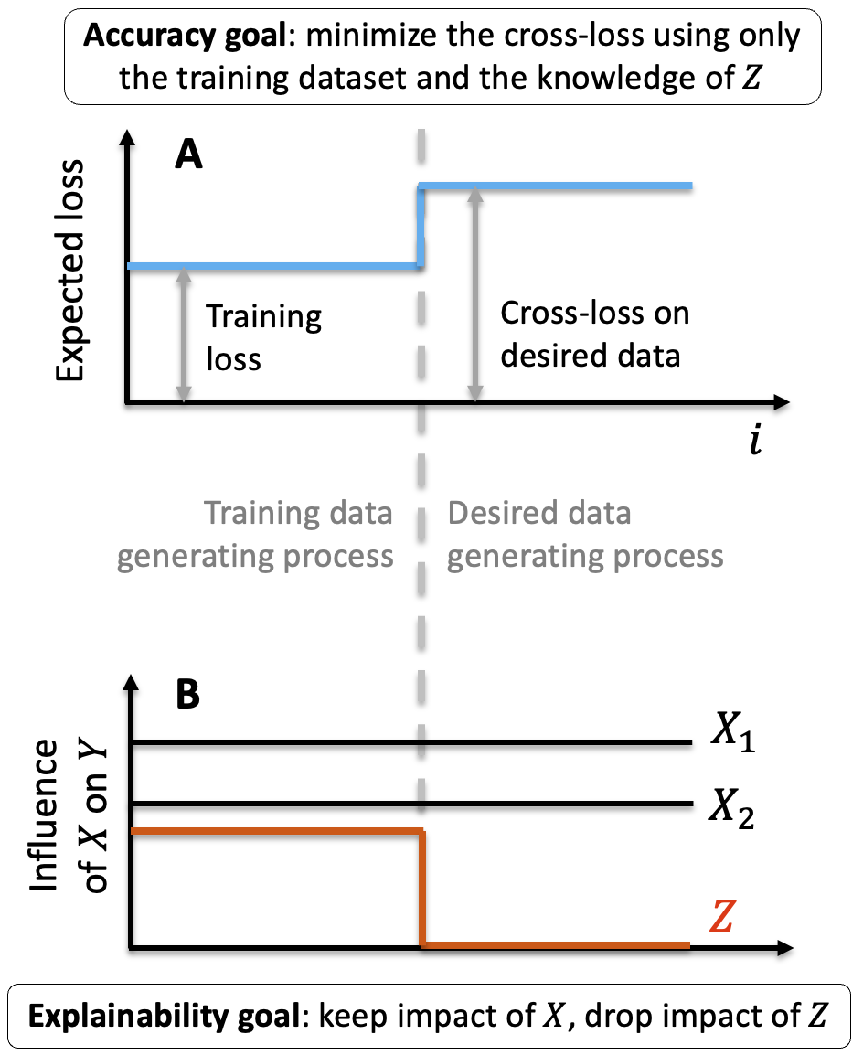
Contributions. To address this problem, independently of the given training data type, we propose that the objective of fair supervised learning methods is to minimize the expected cross-loss, $\operatorname*{\mathbb{E}}_{D_{\text{test}}}[\ell(U,\hat{y}(\bm{X}))]$, on the non-discriminatory test dataset $D_{\text{test}}$ drawn from $P_{\text{test}}(\bm{X},\bm{Z},U)$, while training on a potentially discriminatory data $D_{\text{train}}$ (§3), as in Figure 2A. Achieving that objective may sound infeasible, given lack of any assumptions about the concept shift, but the desideratum that the attribute $\bm{Z}$ shall not directly influence the model outcomes $\hat{Y}$ comes in handy. We show that a learning algorithm averaging probabilistic interventions on the protected attribute optimizes cross-loss under additive directly discriminatory dataset shifts (§4). Such interventions previously were applied to compute explainability measures (Datta et al., 2016; Janzing et al., 2019), and were used in the context of discrimination prevention only recently by our work (Grabowicz et al., 2022). In that study, we proposed that the goal of a fair learning algorithm is to nullify the influence of the protected attribute, while preserving the influence of remaining attributes (the explainability goal in Figure 2), which is achieved by marginal interventional mixtures. In this work, we introduce a novel goal of cross-loss minimization, which is achieved by optimal interventional mixtures, and show that the two methods are equivalent in certain conditions. We evaluate and compare the optimal interventional mixture with the state-of-the-art algorithms addressing discrimination (§5) on synthetic datasets simulating direct discrimination and proxy variables (§6), and on real-world datasets (§7), including those with multiple protected attributes, finding that the optimal interventional mixture leverages parity measures and accuracy, and can accurately recover the unbiased ground truth. The source code of the implementation and evaluation of all methods will be released within an open-source software library upon publication.

2. Related Works

Causal notions of fairness. One can define direct and indirect discrimination as direct and indirect causal influence of $Z$ on $Y$, respectively (Zhang et al., 2017; Zhang and Bareinboim, 2018; Marx et al., 2019). While this notion of direct discrimination is consistent with the concept of disparate treatment in legal systems, the corresponding indirect discrimination is not consistent with them, since the business necessity clause allows the use of an attribute that depends on the protected feature (causally or otherwise), if only the attribute is judged relevant to the decisions made, e.g., as in the seminal court case of Ricci v. DeStefano (Ricci v. DeStefano 557 U.S. 557, Docket No. 07-1428, 2009). This issue is addressed by path-specific notions of causal fairness (Nabi et al., 2019; Chiappa, 2019; Wu et al., 2019). However, if there is no limit on the influence that can pass through fair paths, then the path can be used for inducing discrimination, as in the aforementioned case of redlining. Hence, causal accounts of discrimination do not capture induced discrimination (Kilbertus et al., 2017; Kusner et al., 2017; Zhang and Bareinboim, 2018; Salimi et al., 2019; Nabi et al., 2019; Chiappa, 2019; Wu et al., 2019), which is common in machine learning and is the focus of this work. To address this issue, our recent work defines induced discrimination as a change in the causal influence of non-protected features associated with the protected attributes and proposes a marginal interventional mixture to inhibit direct and induced discrimination (Grabowicz et al., 2022). However, that work does not discuss multiple protect attributes and it does not consider discriminatory concept shifts.

Dataset shifts. There is a growing interest of machine learning community in dataset shifts, since they are surprisingly common in reality and often negatively impact the performance of supervised models on deployment (Koh et al., 2020; Sagawa et al., 2020). The most common dataset shift is a covariate shift, where the distribution of features or decisions changes between the training and test datasets, i.e., $P_{\text{train}}(\bm{x},z)\neq P_{\text{train}}(\bm{x},z)$, or $P_{\text{train}}(y)\neq P_{\text{test}}(y)$, respectively (Moreno-Torres et al., 2012). In the context of fair machine learning, outcome perturbations were first proposed as random swaps of labels in binary classification, i.e., $y\sim\operatorname*{\textit{P}}(y|u)$, where $y$ is a perturbed version of $u$ (Fish et al., 2016). That study, however, assumed no access to the protected attribute, so the random swaps correspond to adding i.i.d. noise in the output variable. Here, we propose to use a different type of dataset shift, known as concept shift, i.e., $P_{\text{train}}(y|\bm{x},z)\neq P_{\text{test}}(y|\bm{x},z)$, to simulate discriminatory perturbations of data and evaluate the resilience of learning methods to such perturbations.

3. Problem formulation

Before we formalize the problem of discrimination prevention based on dataset shifts, we must first define discrimination in the context of decision making. While many other studies focus on statistical notions of fairness (Donini et al., 2018; Woodworth et al., 2017; Hardt et al., 2016; Pleiss et al., 2017; Zafar et al., 2017b; Barocas et al., 2019), our dataset shift-based notions are drawn from abstractions of legal concepts and casual influence notions.

3.1. Fairness and discrimination

Our prior work defined unfair influence and fair relationship between protected attributes $\bm{Z}$ and decisions $Y$ by tying them to legal texts and instruments (Grabowicz et al., 2022).

Definition 0.

Unfair influence is an influence of protected feature(s) $\bm{Z}$ on specified type of decisions $Y$ that is judged illegal via some legal instrument, e.g., Title VII of the U.S. Civil Rights Act of 1964 which states that hiring decisions ($Y$) shall not be influenced by race, color, religion, sex, and national origin ($\bm{Z}$) (Title VII of the Civil Rights Act, 1964).

Definition 0.

Fair relationship of protected feature(s) $\bm{Z}$ with non-protected feature(s) $\bm{X}$ is a relationship that is judged legal in the making decisions of $Y$, e.g., the U.S. business necessity clause.

In real-world contexts, many models can generate decisions $Y$ without directly using the protected attribute $\bm{Z}$, while using non-protected features $\bm{X}$ which may be associated with the protected attribute. Even though these features may be related to the protected attribute, they may be legally admissible for use in the decision-making if they are not unfairly influenced by the protected feature(s), i.e., they are relevant to the decisions and fulfil a business purpose recognized by legal agencies. For instance, in the case of Ricci v. DeStefano (Ricci v. DeStefano 557 U.S. 557, Docket No. 07-1428, 2009), the U.S. Supreme Court ruled that the feature in question, a promotion exam, did not violate business necessity despite its association with race. Thus according to the court, there was a fair relationship between the exam and race.

With these definitions of unfair influence and fair relationship, discrimination can be defined through measures of causal influence. Formal frameworks for causal models include classic potential outcomes (PO) and structural causal models (SCM) (Pearl, 2009). In this notation, the potential outcome for variable $Y$ after intervention $do(\bm{X}=\bm{x},\bm{Z}=\bm{z})$ is written as $Y_{\bm{x},\bm{z}}$, which is the outcome we would have observed had the variables $\bm{X}$ and $\bm{Z}$ been set to the values $\bm{x}$ and $\bm{z}$ via an intervention. It is assumed that there are direct causal links from $\bm{X}$ and $\bm{Z}$ to $Y$, that all variables are observed, and there are no assumptions about the relations between $\bm{X}$ and $\bm{Z}$ and their components. These assumptions hold at the very least for a model $\hat{Y}$ of $Y$ that uses $\bm{X}$ and $\bm{Z}$ as features — this foundational point enables explainability measures, e.g., various feature influence definitions (Janzing et al., 2019). Hence, in our prior work we argue that if the intentions and reasoning behind the development process of the model $\hat{Y}$ was legally admissible, e.g., proxies were not used as a replacement for the protected attribute, then despite the unknowingly incorrect epistemic state represented by the model, e.g., partially incorrect causal representation, legal systems may acquit model developers of discrimination (Grabowicz et al., 2022). Under these assumptions, the causal controlled direct effect on $Y$ of changing the value of $\bm{Z}$ from a reference value $\bm{z}$ to $\bm{z}^{\prime}$ given that $\bm{X}$ is set to $\bm{x}$ (Pearl, 2009) is

(1) $$\text{CDE}_{Y}(\bm{z}^{\prime},\bm{z}|\bm{x})=\operatorname*{\mathbb{E}}[Y_{\bm{x},\bm{z}^{\prime}}-Y_{\bm{x},\bm{z}}].$$

By tying the causal concept of controlled direct effect to the notions of fair influence and unfair relationship, we defined three concepts of discrimination – direct, indirect, and induced (Grabowicz et al., 2022).

Definition 0.

Direct discrimination is an unfair influence of protected attribute(s), $\bm{Z}$, on the decisions $Y$, i.e., $\exists_{z,z^{\prime}}\exists_{\bm{x}}\text{CDE}_{Y}(\bm{z},\bm{z}^{\prime}|\bm{x})\neq 0$.

Definition 0.

Indirect discrimination is an influence on the decisions $Y$ of feature(s) $\bm{X}$ whose relationship with $\bm{Z}$ is not fair, i.e., $\exists_{x,x^{\prime}}\exists_{\bm{z}}\text{CDE}_{Y}(\bm{x},\bm{x}^{\prime}|\bm{z})\neq 0$.

Definition 0.

Discrimination induced via $X_{i}$ is a transformation of the process generating $U$ into a new process generating $Y$ that modifies the influence of certain $X_{i}$ depending on $\bm{Z}$ between the processes $U$ and $Y$, i.e., $\exists_{\bm{z}}\exists_{\bm{x},\bm{x}^{\prime}}\text{CDE}_{U}(\bm{x},\bm{x}^{\prime}|\bm{z})\neq\text{CDE}_{Y}(\bm{x},\bm{x}^{\prime}|\bm{z})$ given that $P(\bm{x}|\bm{z})\neq P(\bm{x})$ or $P(\bm{x}^{\prime}|\bm{z})\neq P(\bm{x}^{\prime})$.

To remove direct discrimination, one can construct a model $\hat{Y}$ that does not use $\bm{Z}$. However, the removal of direct discrimination may induce discrimination indirectly via the attributes $X_{i}$ with an unfair relationship with the protected attributes $\bm{Z}$, even if there is no causal link from $\bm{Z}$ to $X_{i}$. Therefore, we propose that methods inhibiting discrimination shall do so without inducing discrimination.

Example 0.

Consider a hypothetical linear model of loan interest rate, $Y$. Using similar models, prior works suggest that interest rates differ by race, $Z$ (Turner and Skidmore, 1999; Bartlett et al., 2019). Some loan-granting clerks may produce non-discriminatory decisions, $u=\beta_{0}-x_{1}$, while other clerks may discriminate directly, $y_{\text{dir}}=\beta_{0}-x_{1}+z$, where $\beta_{0}$ is a fixed base interest rate, $x_{1}$ is a relative salary of a loan applicant, while $z$ encodes race and takes some negative (positive) value for White (non-White) applicants. If the protected attribute is not available, e.g., loan applications are submitted online, then a discriminating clerk may induce discrimination in the interest rate, by using a proxy for race, $y_{\text{ind}}=\beta_{0}-x_{1}+x_{2}$, where $x_{2}$ is the proxy, e.g., an encoding of the zip code (as in the redlining) or the first name (as in the seminal work of Bertrand and Mullainathan) of the applicant.

3.2. Discriminatory concept shifts

Distinct from our prior work, we introduce an additional goal in discrimination prevention from the perspective of dataset shifts. That is, we propose to use discriminatory perturbations dependent on the protected attribute to simulate a concept shift, i.e., $P_{\text{train}}(y|\bm{x},z)\neq P_{\text{test}}(y|\bm{x},z)$, and to evaluate the cross-loss of learning methods w.r.t. to such concept shifts (Moreno-Torres et al., 2012) (explainability goal in Figure 2). These concept shifts reflect bias in a historical data-generating process, rather than a sampling bias which typically is associated with covariate shifts.

Definition 0.

Discriminatory concept shift is a transformation of the process generating $U$ that is not affected by any discrimination into a new process generating $Y$ that is affected by direct discrimination.

Example 0.

We continue the example of the loan interest rate. The transformation from $u=\beta_{0}-x_{1}$ to $y_{\text{dir}}=\beta_{0}-x_{1}+z$ via a directly discriminatory additive perturbation of $z$ (race) is a discriminatory concept shift. This gives two datasets, $\tilde{D}=\{(x_{1}^{i},x_{2}^{i},z^{i},y_{\text{dir}}^{i})\}$ for training and $D=\{(x_{1}^{i},x_{2}^{i},z^{i},u^{i})\}$ for testing.

We do not assume that the perfectly fair decision-making process, illustrated in Figure 1A, exists already in all real-world contexts. In stark contrast, we posit that its knowledge shall not be required to prevent discrimination in supervised learning. The above constructs enable us to formalize the goal for fair learning methods on the grounds of dataset shifts and specify the idealized real-world scenarios that the methods achieving this goal address. Next, we define the cross-loss of a supervised learning algorithm to discriminatory concept shifts, which measure how well an algorithm trained on potentially discriminatory training dataset, i.e., $D_{\text{train}}=\tilde{D}$ or $D_{\text{train}}=D$, performs when it is evaluated on a non-discriminatory $D_{\text{test}}=D$.

Definition 0.

Cross-loss. The solution of supervised learning algorithm $a$, $\hat{y}_{a}(\bm{x}|\tilde{D})$, is a model obtained by training on the potentially discriminatory dataset $\tilde{D}$. The empirical cross-loss function is an expected loss of this model w.r.t. the non-discriminatory data $D$, $\operatorname*{\mathbb{E}}_{D}\left[\ell\left(U,\hat{y}_{a}(\bm{X}|\tilde{D})\right)\right].$

The cross-loss measures how well the model learned by an algorithm training on the discriminatory data predicts the fair data, i.e., how well it performs under a discriminatory concept shift.

Example 0.

We continue the example of the loan interest rate. For simplicity, assume that all variables have zero mean, no correlation between $X_{1}$ and $Z$, and a positive correlation $r>0$ between $X_{2}$ and $Z$. Let the training dataset be $\tilde{D}=\{(x_{1},x_{2},z,y_{\text{dir}})\}$. If we applied standard supervised learning under the quadratic loss, then we would learn the model $\hat{y}_{1}=\beta_{0}-x_{1}+z$, which is directly discriminatory and results in high cross-loss $\operatorname*{\mathbb{E}}_{D}\left[\ell\left(U,\hat{y}_{1}(\bm{X}|\tilde{D})\right)\right]=\operatorname*{\mathbb{E}}_{Z}Z^{2}$. If we dropped the protected attribute, $Z$, before regressing $Y_{\text{dir}}$ on the attributes $X_{1}$ and $X_{2}$, then we would learn the model $\hat{y}_{2}=\beta_{0}-x_{1}+rx_{2}$, which also yields a sub-optimal cross-loss, $\operatorname*{\mathbb{E}}_{D}\left[\ell\left(U,\hat{y}_{2}(\bm{X}|\tilde{D})\right)\right]=r^{2}\operatorname*{\mathbb{E}}_{X_{2}}X_{2}^{2}$, that increases with $r$ due to the growing discrimination induced via $X_{2}$.

4. Optimal interventional mixture

Next, we introduce a supervised learning method based on probabilistic interventions that aims to prevent direct discrimination in $Y$ without inducing any discrimination. We prove that it minimizes cross-loss, up to a constant, under the assumption of the concept shift coming from additive direct perturbations (§4.1). In addition, if $Y$ is impacted by indirect discrimination, i.e., $\bm{Z}$ unfairly influences $\bm{X}$, we can address it as direct discrimination in $\bm{X}$. To prevent indirect discrimination one can apply our method in a nested way (§4.2) that resembles the path-specific counterfactual fairness (Chiappa, 2019).

4.1. Removal of direct discrimination

The proposed method is a post-processing approach and has two optimisation steps. In the first step, we train the model $\hat{y}(\bm{x},z)$ using all features, both protected $Z$ and relevant $\bm{X}$, without any consideration of fairness, by minimizing the corresponding expected loss $\operatorname*{\mathbb{E}}_{D_{\text{train}}}[\ell(Y,\hat{y}(\bm{X}))]$. Most importantly, the protected attribute is available during the training, so the model does not need to use third variables as surrogates of the protected attribute, thus avoiding inducing discrimination via $\bm{X}$ (we provide theoretical and empirical evidence for this statement in Proposition 2 and Section 6.1, respectively). In this way, we aim to estimate the values of model parameters while avoiding bias introduced by the discriminatory concept shift. These parameters regulate the impact of the relevant variables $\bm{X}$ on $Y$. In the second step, we eliminate the influence of the protected attribute. This is achieved by intervening probabilistically on the full model trained with all features and mixing the interventions on the protected attribute via a mixing distribution $\pi(Z^{\prime})$ that is independent from other variables, yielding $\hat{y}_{\pi}(\bm{x})=\sum_{z^{\prime}}\hat{y}(\bm{x},z^{\prime})\pi(z^{\prime})dz^{\prime}$. Methods preventing discrimination trade accuracy to fulfill fairness objectives (Zafar et al., 2017b). Here, we search for the optimal mixing distribution, $\pi^{*}(z^{\prime})$, that minimizes the expected loss, $\operatorname*{\mathbb{E}}_{D_{\text{train}}}[\ell(Y,\hat{y}_{\pi}(\bm{X}))]$, while all parameters of the full model $\hat{y}(\bm{x},z)$ are fixed, i.e., $\pi^{*}=\operatorname*{arg\,min}_{\pi}\operatorname*{\mathbb{E}}_{D_{\text{train}}}[\ell(Y,\hat{y}_{\pi}(\bm{X}))].$ This optimization problem is convex for quadratic and negative log-likelihood loss functions. Thus, the optimal weighting distribution can be found by applying disciplined convex programming with constraints ensuring that $\pi(z^{\prime})$ is a distribution, i.e., $\sum_{z^{\prime}}\pi(z^{\prime})=1$ and $\pi(z^{\prime})\geq 0$ for all $z^{\prime}$ (Diamond and Boyd, 2016). Once the optimal mixing distribution is known, the optimal interventional mixture (OIM) can be computed, $\hat{y}^{*}(\bm{x})=\sum_{z^{\prime}}\hat{y}(\bm{x},z^{\prime})\pi^{*}(z^{\prime})dz^{\prime},$ which constitutes the solution of the proposed learning algorithm.

Unlike many methods achieving statistical fairness objectives, our method is seamlessly applicable to scenarios with multiple protected attributes or numeric attributes such as age. This is accomplished by mixing the interventions on all combinations of the protected attributes in the second optimization step. Next, for discriminatory data transformations that have a simple additive form, i.e., $y=u+h(z)$, we prove that optimal interventional mixture minimizes cross-loss on non-discriminatory data and show that for L2 loss the accuracy and explainability goals (Figure 2) of fair machine learning lead to the same fair models.

Proposition 0.

Let the non-discriminatory data have $u=f(\bm{x})+\nu$ and the data following a discriminatory concept shift have $y=f(\bm{x})+h(\bm{z})+\nu$, where $f$ and $h$ are some functions and $\nu$ is i.i.d. noise independent from $\bm{X}$ and $Z$. Assume that the same $\ell^{p}$ loss, either $\ell^{1}$ or $\ell^{2}$, is used for model learning and the computation of resilience. If the estimation model is well specified w.r.t. the discriminatory data-generating process and the estimation method is consistent, then the OIM, asymptotically with the number of samples, is $\hat{y}^{*}(\bm{x})=f(\bm{x})+C_{p}$, and it minimizes the expected cross loss $\operatorname*{\mathbb{E}}_{D}\left[\ell\left(U,\hat{y}_{a}(\bm{X}|\tilde{D})\right)\right]$ up to the constant $C_{p}$ that depends on the unknown $h(\bm{Z})$.

Example 0.

We continue the example of a model for loan interest rate. The full model is $\hat{y}(\bm{x},\bm{z})=\beta_{0}-x_{1}+\bm{z}$. The optimal interventional mixture is $\hat{y}^{*}=\beta_{0}-x_{1}+\beta_{\pi}$, where the intercept $\beta_{\pi}$ is the result of mixing over the optimal $\pi^{*}(z^{\prime})$. In this case, $\beta_{\pi}=\operatorname*{\mathbb{E}}_{Z}Z=0$ due to the optimization. Thus, the algorithm recovers the non-discriminatory ground truth.

The proof follows from the definition of consistent estimator (see full proof in Appendix A). For a particular dataset that does not meet the condition $C_{p}=0$, one can propose a better model than the OIM by subtracting $C_{p}$ from model’s intercept, which is a sum of $C_{p}$ and a component of $f(x)$, but $C_{p}$ depends on the unknown $h(Z)$ and, without knowing $h(Z)$, we do not know what to subtract, so a learning strategy that improves the resilience does not exist. Furthermore, the case of nonzero $C_{p}$ is practically irrelevant, because it represents a data perturbation that affects all individuals in the same way, e.g., it introduces across the board more positive outcomes $y$ without changing their dependence on $\bm{x}$, i.e., $\operatorname*{\mathbb{E}}[Y|\bm{x}]=\operatorname*{\mathbb{E}}[U|\bm{x}]+C_{p}$. The above proposition is valid for well-specified models. Next, we prove analogue result for universal approximators such as deep learning models.

Corollary 0.

Let the same assumptions hold as in Proposition 1, but this time the estimation model is a universal approximator. Then the OIM is an arbitrarily close approximation of $f(\bm{x})+C_{p}$, which according to Proposition 1 minimizes the expected loss $\operatorname*{\mathbb{E}}_{D}\left[\ell\left(U,\hat{y}_{a}(\bm{X}|\tilde{D})\right)\right]$ up to $C_{p}$.

The proof follows from universal approximator theorems and Proposition 1 (see Appendix A). These guarantees do not universally hold for our prior work, which is the only work that proposes a similar interventional mixtures for inhibiting discrimination (Grabowicz et al., 2022). Rather than finding an optimal mixture, we previously proposed to utilize the marginal distribution of the protected attribute to build a marginal interventional mixture, i.e., $\hat{y}_{\text{MIM}}(\bm{x})=\operatorname*{\mathbb{E}}_{\bm{Z}}[\hat{y}(\bm{x},\bm{Z})]$.

Proposition 0.

Let the same assumptions hold as in Proposition 1. Then the marginal interventional mixture (MIM), asymptotically with the number of samples, is $\hat{y}_{\text{MIM}}(\bm{x})=\operatorname*{\mathbb{E}}_{\bm{Z}}[\hat{y}(\bm{x},\bm{Z})]=f(\bm{x})+\operatorname*{\mathbb{E}}[h(Z)+\nu]$, and minimizes the expected cross loss $\operatorname*{\mathbb{E}}_{D}\left[\ell\left(U,\hat{y}_{a}(\bm{X}|\tilde{D})\right)\right]$ only for $\ell^{2}$ loss up to the constant $\operatorname*{\mathbb{E}}[h(\bm{Z})+\nu]$.

4.2. Removal of indirect discrimination via optimal counterfactual mixture

In real-world scenarios, a non-protected feature, $X_{i}$, can be unfairly influenced by $\bm{Z}$. If decisions $Y$ used such an $X_{i}$, then $Y$ would face indirect discrimination. To prevent this, one can apply a nested multi-stage version of OIM. More precisely, say that we have $X_{1}$, $X_{2}$, and $\bm{Z}$, where $X_{1}$ is unfairly influenced by $\bm{Z}$, and all are used by decisions $Y$. We first create a model $\hat{Y}$ using $X_{1}$, $X_{2}$, and $\bm{Z}$. Then, we create a model $\hat{X}_{1}$, using $X_{2}$ and $\bm{Z}$ and other relevant features that we have access to, and apply the OIM to create a “fair” model $\hat{X}_{1}^{*}$. Lastly, to create $\hat{Y}^{*}$, we replace $X_{1}$ with $\hat{X}_{1}^{*}$, learn $\hat{Y}$, and apply the OIM. This is a reasonable solution, but in situations where we know the value of a variable for which we apply OIM, such as $X_{1}$ here, we can do better via counterfactual analysis.

4.2.1. Counterfactual mixtures.

Causality literature posits a causal hierarchy and distinguishes between interventional and counterfactual estimates (Pearl et al., 2016). The latter differ from former in that they assume that everything stays the same, including any exogenous noise values, when estimating the effect of an intervention. Note that the interventional mixture calculates the value of $\hat{X}_{1}$ had the casual influence of $\bm{Z}$ been removed from it given the values of all observed variables, but not the values of exogenous noise. However, each variable can contain exogenous noise, i.e., unobserved intrinsic noise not associated with any other variable. In the situations where we know the value of the variable for which we want to develop a fair model, we can use that value to infer that variable’s exogenous noise. For such situations, we propose an optimal counterfactual mixture (OCM), which merges the three canonical counterfactual reasoning steps with the OIM step: (abduction) infer exogenous noise for a variable, (intervention) apply the OIM to remove the influence of the protected attribute on that variable, and (counterfactual prediction) estimate the counterfactual value of the variable given the exogenous noise and intervention.

4.2.2. Counterfactual mixtures comparison.

We compare the interventional (OIM) and counterfactual (OCM) versions of our method as well as the related path-specific counterfactual fairness (PSCF) using a multi-stage linear model introduced in the PSCF paper (Chiappa, 2019):

(2) $$M =\theta^{m}+\theta^{m}_{z}Z+\theta^{m}_{c}C+\epsilon_{m},$$

(3) $$L =\theta^{l}+\theta^{l}_{z}Z+\theta^{l}_{c}C+\theta^{l}_{m}M+\epsilon_{l},$$

(4) $$Y =\theta^{y}+\theta^{y}_{z}Z+\theta^{y}_{c}C+\theta^{y}_{m}M+\theta^{y}_{l}L+\epsilon_{y},$$

where $C$, $M$, $L$ are components of $\bm{X}$, $\bm{Z}$ is the protected attribute, and $\epsilon_{c}$, $\epsilon_{m}$, $\epsilon_{l}$ are exogenous noise variables. The causal influence of $Z$ on decisions $Y$ and the mediator $M$ is assumed unfair and all other influences are fair. In other words, $Y$ is affected by direct discrimination via $Z$ and indirect discrimination via $M$. This means that our method needs to be applied first to $M$ and then to $Y$.

For simplicity, without loss of generality, let us consider a scenario where we have enough samples to have perfect estimates of a well-specified model’s parameters, so that the estimated model is $\hat{m}=\theta^{m}+\theta^{m}_{z}z+\theta^{m}_{c}c$. In this scenario, the abduction step corresponds to computing $\epsilon_{m}=m-\hat{m}$, the intervention step to applying OIM to $\hat{m}$, yielding $\hat{m}^{*}=\theta^{m}+\theta^{m}_{z}z^{*}+\theta^{m}_{c}c$, and the counterfactual prediction to injecting the abducted noise into the estimated model, $\hat{m}^{c}=\theta^{m}+\theta^{m}_{z}z^{*}+\theta^{m}_{c}c+\epsilon_{m}$. Overall, we refer to these three steps as the single-stage OCM. Same as the PSCF, the multi-stage OCM corrects the decision through a correction on all the variables that are influenced by the protected attribute along unfair pathways. Thus, we first apply the OCM to get a non-discriminatory counterfactual $\hat{m}^{\text{c}}$, then we propagate $\hat{m}^{\text{c}}$ to its descendants and apply the OCM to yield a fair counterfactual $\hat{l}^{\text{c}}$, and finally we propagate the two counterfactuals to $\hat{y}$ and apply the OIM (not OCM, since we do not observe $Y$) to get $\hat{y}^{\text{c}}$:

(5) $$\hat{m}^{\text{c}} =\theta^{m}+\theta^{m}_{z}z^{*}+\theta^{m}_{c}c+\epsilon_{m}=m-\theta^{m}_{z}(z-z^{*}),$$

(6) $$\hat{l}^{\text{c}} =\theta^{l}+\theta^{l}_{z}z+\theta^{l}_{c}c+\theta^{l}_{m}\hat{m}^{\text{c}}+\epsilon_{l}=l-\theta_{m}^{l}(m-\hat{m}^{\text{c}}),$$

(7) $$\hat{y}^{\text{c}} =\theta^{y}+\theta^{y}_{z}z^{*}+\theta^{y}_{c}c+\theta^{y}_{m}\hat{m}^{\text{c}}+\theta^{y}_{l}\hat{l}^{\text{c}},$$

where $z^{*}$ is the expected value of Z resulting from the optimal mixing distribution for $Z$. Conversely, applying solely the OIM to obtain $\hat{m}^{*}$, $\hat{l}^{*}$, and $\hat{y}^{*}$ does not take advantage of estimating the noise terms $\epsilon_{m}$ and $\epsilon_{l}$, and results in estimators

(8) $$\hat{m}^{\text{*}} =\theta^{m}+\theta^{m}_{z}z^{*}+\theta^{m}_{c}c,$$

(9) $$\hat{l}^{\text{*}} =\theta^{l}+\theta^{l}_{z}z+\theta^{l}_{c}c+\theta^{l}_{m}\hat{m}^{\text{*}},$$

(10) $$\hat{y}^{\text{*}} =\theta^{y}+\theta^{y}_{z}z^{*}+\theta^{y}_{c}c+\theta^{y}_{m}\hat{m}^{\text{*}}+\theta^{y}_{l}\hat{l}^{\text{*}}.$$

When comparing $\hat{y}^{*}$ and $\hat{y}^{\text{c}}$ we observe that difference in estimating $\epsilon_{m}$ unsurprisingly yields the noise terms, $\hat{y}^{\text{c}}=\hat{y}^{*}+\theta^{y}_{m}\epsilon_{m}+\theta^{y}_{l}\theta^{l}_{m}\epsilon_{m}$, which results in a larger error w.r.t. $Y$ for the OIM than the OCM,

(11) $$\operatorname*{\mathbb{E}}(Y-\hat{Y}^{*})^{2}=\operatorname*{\mathbb{E}}(Y-\hat{Y}^{\text{c}})^{2}+(\theta^{y}_{m}\epsilon_{m}+\theta^{y}_{l}\theta^{l}_{m}\epsilon_{m})^{2}.$$

A comparison with the PSCF reveals that $\hat{y}^{\text{c}}=\hat{y}^{\text{PSCF}}+\Delta$, where $\Delta=z^{*}(\theta^{y}_{z}+\theta^{y}_{m}\theta^{m}_{z}+\theta^{y}_{l}\theta^{l}_{m}\theta^{m}_{z})$. In fact, the mean squared error w.r.t. $Y$ is larger for the PSCF than for the OCM by the square of the difference, i.e., $\operatorname*{\mathbb{E}}(Y-\hat{Y}^{\text{PSCF}})^{2}=\operatorname*{\mathbb{E}}(Y-\hat{Y}^{c})^{2}+\Delta^{2}$. Overall, the OCM is more accurate than the PSCF, because the PSCF relies on a choice of reference value, $z^{\prime}$, also known as baseline, which is assumed $z^{\prime}=0$ in the PSCF paper and above example. However, this choice is arbitrary and it is not clear what the baseline should be for non-binary $\bm{Z}$. By contrast, the OCM introduces a distribution $\pi(z^{\prime})$ and optimizes it for accuracy. In addition, it follows from Proposition 1 and Corollary 1, that the OIM and by extension the OCM, are the most accurate interventional and counterfactual models on the non-discriminatory test datasets (up to the unlearnable constant $C_{p}$).

5. Evaluation method and evaluated methods

In the remaining sections, we measure the “resilience” of various learning methods to discriminatory concept shifts that have more complex functional forms than the additive shifts described in the previous section. We begin by introducing the notion of resilience and the evaluated learning methods addressing discrimination.

5.1. Resilience

Note that the range of cross-loss values depends on the dataset and loss function. To make comparisons across datasets, we introduce the measure of resilience by normalizing the inverse of cross-loss, so that the resilience is a number between 0 and 1. For a specific pair of datasets $\tilde{D}$ and unknown $D$, the larger the cross-loss, the lower the resilience of the learning algorithm to the concept shift from training data $\tilde{D}$.

Definition 0.

Resilience. The resilience of algorithm $a$ to a discriminatory concept shift from non-discriminatory data $D$ to $\tilde{D}$ is a ratio of the expected loss of the standard algorithm training on $D$ and the cross-loss of algorithm $a$ training on $\tilde{D}$:

(12) $$\Omega_{a}=\operatorname*{\mathbb{E}}_{D}\left[\ell\left(U,\hat{u}(\bm{X}|D)\right)\right]/\operatorname*{\mathbb{E}}_{D}\left[\ell\left(U,\hat{y}_{a}(\bm{X}|\tilde{D})\right)\right],$$

where $\hat{u}(\bm{x}|D)$ is a model of the non-discriminatory ground truth trained on dataset $D$.

The enumerator of resilience takes into account that $U$ can be intrinsically random and unpredictable. The resilience is confined, $0\leq\Omega\leq 1$. This property is ensured if both learning algorithms yielding the models $\hat{u}(\bm{x}|D)$ and $\hat{y}_{a}(\bm{x}|\tilde{D})$ optimise the same vanilla objective function, e.g., both optimize expected loss, where the algorithm $a$ adds an extra component to address discrimination. An algorithm that is perfectly resilient to the discriminatory concept shift yields $\Omega=1$, and $\Omega=0$ otherwise.

5.2. Evaluated learning methods

A number of algorithms addressing discrimination have been developed by adding a constraint or a regularization to the objective function (Pedreshi et al., 2008; Feldman et al., 2014; Zafar et al., 2015, 2017b; Hardt et al., 2016; Zafar et al., 2017c; Woodworth et al., 2017; Pleiss et al., 2017; Donini et al., 2018). Most of these algorithms prevent direct discrimination, but it should come as no surprise that some of them do not prevent the induction of discrimination. For instance, the algorithms that put constraints on the aforementioned disparities in treatment and impact (Pedreshi et al., 2008; Feldman et al., 2014; Zafar et al., 2015) induce “reverse” discrimination, by affecting the members of advantaged group and the people similar to them in a non-desirable manner when training on a non-discriminatory dataset $D$ (Lipton et al., 2018). As an example, such “reverse” discrimination would result in a situation where there is less job opportunities for similarly qualified short-haired women than long-haired women, because short hair is associated with males and there is a historical correlation between hiring and gender (Lipton et al., 2018). Other studies propose interesting statistical notions of fairness, such as equalized opportunity, $\operatorname*{\textit{P}}(\hat{y}|y=1,z=0)=\operatorname*{\textit{P}}(\hat{y}|y=1,z=1)$, equalized odds, $\operatorname*{\textit{P}}(\hat{y}|y,z=0)=\operatorname*{\textit{P}}(\hat{y}|y,z=1)$ (Donini et al., 2018; Woodworth et al., 2017; Hardt et al., 2016; Pleiss et al., 2017), or parity mistreatment, i.e., $\operatorname*{\textit{P}}(\hat{y}\neq y|z=0)=\operatorname*{\textit{P}}(\hat{y}\neq y|z=1)$ (Zafar et al., 2017b). However, prior works reveals the impossibility of simultaneously satisfying multiple non-discriminatory objectives, such as equalized opportunity and parity mistreatment (Chouldechova, 2017; Kleinberg et al., 2017; Friedler et al., 2016). There is a need to compare them.

We evaluate several of such methods in the next section. For this evaluation, we select a diverse set of algorithms that aim to prevent discrimination through different objectives: disparate impact (Zafar et al., 2015; Zafar et al., 2017a), disparate mistreatment (Zafar et al., 2017b), preferential fairness (Zafar et al., 2017c), equalized odds (Hardt et al., 2016), a convex surrogate of equalized odds (Donini et al., 2018), game-theoretic envy-freeness (Zafar et al., 2017c), and a causal database repair  (Salimi et al., 2019). In all cases but one, we use implementations of these algorithms as provided by the authors. We re-implemented one of these methods (Zafar et al., 2015) so that it works for the case of continuous $Y$, since all these methods were originally implemented for the case of discrete decisions $Y$. For the method by Donini et al. (2018) we report the performance with a linear-kernel SVM; the regularization parameter $C$ for was tuned via grid search with $C\in\{0.01,0.1,1\}$. For (Zafar et al., 2017b) we report results for when the model is set to equalize misclassification rates between two groups. For (Zafar et al., 2015) we set the constraint $c=0$. We also evaluate a scenario where we prevent discrimination over multiple protected attributes. Here, the only fair-learning method we evaluate against is the method introduced in the fairness gerrymandering paper (Kearns et al., 2018), as it considers fairness, based on the best subgroup-fair distribution over classifiers, across infinitely many subgroups. For this method, we choose the $\gamma=0.3$ which resulted in an accuracy within a few percentile of traditional learning. The implementation of the methods we used for our experiments (Zafar et al., 2015, 2017b; Zafar et al., 2017c; Hardt et al., 2016; Donini et al., 2018; Kearns et al., 2018) are readily available online.

6. Evaluation on synthetic data

In the synthetic setting, we generate random non-discriminatory datasets $D$, containing samples of $U$, and perform a concept shift to create datasets $\tilde{D}$, containing samples of $Y$. Then, datasets $\tilde{D}$ are used for training, datasets $D$ are used for testing, and we measure the resilience and the feature influence of various learning algorithms preventing discrimination, including the OIM. Next, we make these measurements as a function of the correlation between the protected and non-protected attributes, which often causes learning algorithms to induce discrimination via association. We also study the setting where there is no discriminatory concept shift, but there is a feature correlated with the protected attributes that is fair to use, i.e., permitted by law. Other scenarios where we randomize the parameters of our data generating process or have a discriminatory concept shift under a complex non-linear functional form are available in Appendix D and G, respectively, and yield qualitatively the same results for resilience.

6.1. Resilience captures induced discrimination

Data generation. Without loss of generality, the data generating process of $U$ can yield $\operatorname*{\mathbb{E}}[U|\bm{x}]=\sigma(f(\bm{x}))$, where $f$ is a potentially non-linear function, and $\sigma$ is a function establishing the respective support for $U$. For instance, for classification problems $\sigma$ can be a logistic or softmax function, while for regression it can be identity. Next, we simulate discrimination as a concept shift from $U$ that in general can be represented as $\operatorname*{\mathbb{E}}[Y|\bm{x}]=\sigma(g(\bm{x},z))$, where $g$ is some function. These concept shifts may or may not be discriminatory, depending on how expected outcomes were shifted: i) no discrimination, if $g(\bm{x},z)=f(\bm{x})$, ii) direct discrimination, if $g(\bm{x},z)$ depends on $z$, iii) induced discrimination, if $g(\bm{x},z)=\tilde{f}(\bm{x})\neq f(\bm{x})$. We study simple forms of $f(\bm{x})$ and $g(\bm{x},z)$ that are linear combinations of its arguments, i.e., $f(\bm{x})=\bm{\alpha}^{\intercal}\bm{x}$ and $g(\bm{x},z)=\bm{\tilde{\alpha}}^{\intercal}\bm{x}+\beta z$, and $\sigma$ is the logistic function.

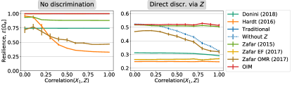
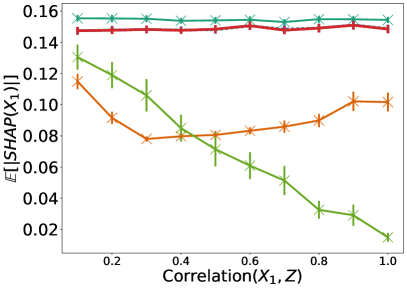
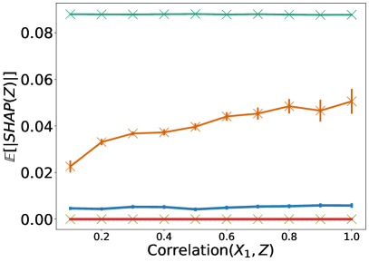
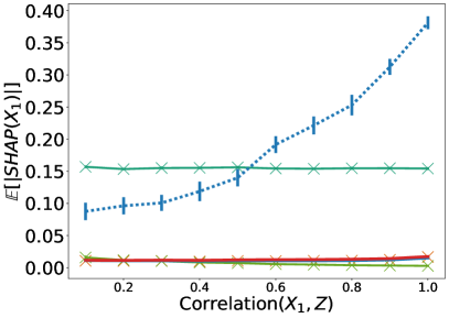
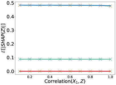
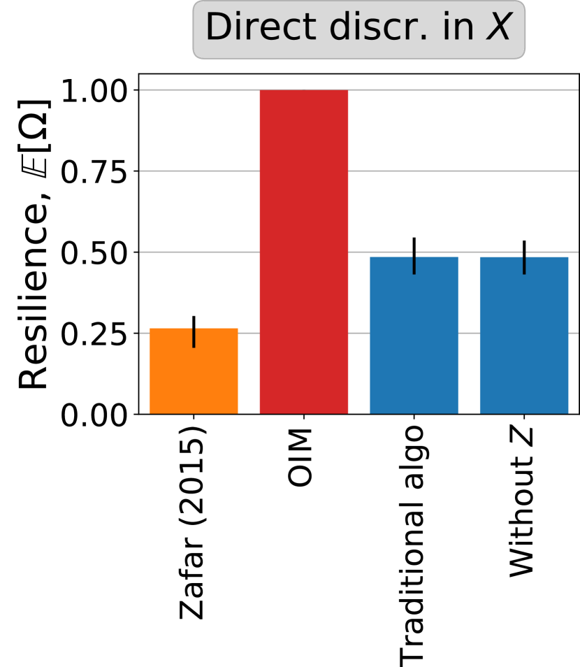
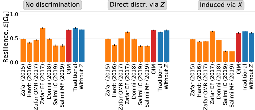
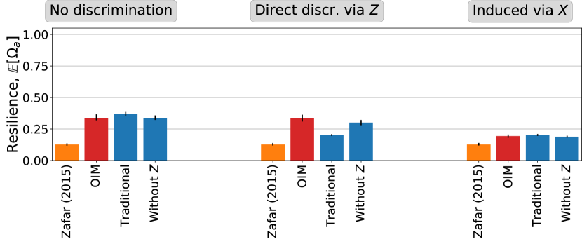
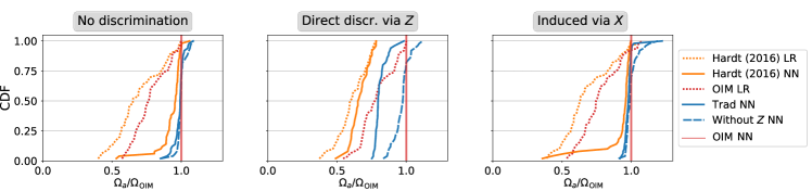
Results. We focus first on a data-generating process that extends the loan-interest Example to binary dependent variables, which are prevalent in real-world decision-making. Specifically, $u\sim\text{Bernoulli}[\operatorname*{\mathbb{E}}[U|\bm{x}]]$ and $y\sim\text{Bernoulli}[\operatorname*{\mathbb{E}}[Y|\bm{x}]]$, where $f(\bm{x})=x_{1}$ and $g(\bm{x},z)=x_{1}+\beta z$. We model this data with logistic regression and measure how the resilience and the expected value of influence of each feature changes with the increasing correlation between $X_{1}$ and $Z$. We measure influence using SHAP (SHapley Additive exPlanations), a popular explainability measure (Lundberg and Lee, 2017).

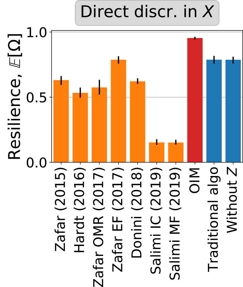
We study two cases of the training dataset $\tilde{D}$: (i) without any concept shift (no discrimination with $\beta=0$, left Figures 3 & 4) and (ii) with a discriminatory concept shift ($\beta=5$, right Figures 3 & 4). In both cases, the resilience of most learning algorithms is sub-optimal and for several methods it drops with the correlation. For case (i), Lipton et al. (2018) demonstrates that the algorithms fighting the disparities in treatment and impact (Pedreshi et al., 2008; Feldman et al., 2014; Zafar et al., 2015) induce “reverse” discrimination. Our measurements of resilience and influence captures this result and extend it to methods based on equalized odds and disparate mistreatment (the orange and brown lines in the left Figure 3 and orange line in Figures  4a), including methods equalizing overall misclassification rate, false negative rate, and related measures (Appendix C). The only methods that do not bias the models in this scenario are: traditional supervised learning and the two methods that fall back to it if there is no direct discrimination in the data, i.e., the game-theoretic method based on envy-freeness (the yellow line is underneath the red line in the left Figure 3) and the OIM. For case (ii), we observe that the resilience of three algorithms decreases with the correlation, suggesting that they induce discrimination via association (Wachter, 2019), i.e., they replace the protected attribute with its proxy, which causes a drop in resilience (e.g., the blue dotted line in the right Figure 3 & in Figure 4b). Therefore, it is not sufficient to simply drop the protected attribute in traditional learning. A real-world example of this phenomenon is “redlining”, where a bank uses a zip code as a replacement for race, whose use is prohibited. Some methods perform poorly irrespective of the correlations, e.g., “Hardt”, because it allows direct discrimination (orange lines in Figure 3 & 4). Overall, the two cases show that many learning algorithms induce discrimination or directly discriminate, i.e., they yield biased models by changing the impact of $\bm{X}$ on $\hat{Y}$ or are directly impacted by $\bm{Z}$.

Figure 3. Average resilience to potentially discriminatory concept shifts decreases with the correlation between $X_{1}$ and $Z$. The coefficient that scales the discrimination in the training data is $\beta=0$ for the case of no discrimination (left) and $\beta=5$ for direct discrimination (right). Each point is an average over 100 random datasets. Error bars show $95\%$ confidence intervals.

(a) No direct discrimination, $g(\bm{x},z)=x_{1}+0*z$

(b) Directly discriminatory, $g(\bm{x},z)=x_{1}+5*z$

Figure 4. Average absolute value of SHAP values for $X_{1}$ and $Z$ as the correlation between $X_{1}$ and $Z$ increases. Each point is an average over 100 random datasets. Error bars show $95\%$ confidence intervals.

7. Evaluation on real-world datasets

In the synthetic settings, we experimented in an idealized environment where we had full information on the discriminatory concept shift and, therefore, knew the non-discriminatory ground truth. However, with real-world scenarios it is often the case that we only have access to a potentially discriminatory dataset without any information about the concept shift or we have a concept shift under a complex non-linear function. Therefore, we analyze the OIM in two types of real-world settings. Firstly, on tabular datasets commonly found in algorithmic fairness research where we have multiple protected attributes and no information on the concept shift. Then, on the CelebA image dataset (Liu et al., 2015) where we have non-discriminatory labels and introduce a discriminatory concept shift, while working with a highly non-linear deep neural net.

Figure 5. Performance of learning algorithms inhibiting discrimination over COMPAS and German Credit datasets. Higher accuracy (ACC) and lower demographic disparity (DD), positive predictive disparity (PPD), and false positive disparity (FPD) are better.

Figure 6. Performance of learning algorithms inhibiting discrimination over all combinations of race & sex on COMPAS. Disparity measures are on each given group w.r.t. Black Males. Higher accuracy (ACC) and lower disparities (DD, PPD, FPD) are better.

7.1. Concept shift information unknown

Datasets. We focus on two datasets that are prevalent in the literature on fairness: the COMPAS dataset of recidivism risk (Larson et al., 2016) and the German Credit dataset of creditworthiness (Dua and Graff, 2017), and their respective binary classification tasks.

The ProPublica COMPAS dataset (Larson et al., 2016) contains the records of 7214 offenders in Broward County, Florida in 2013 and 2014. As target, $y$, we use the binary label describing whether an individual recommitted a crime after being released. For comparison with the original study (Larson et al., 2016), we follow their labeling of recidivism as the positive outcome. In our single-protected attribute scenario we use the race (African American, Caucasian) as the protected feature, $Z$. We use race and sex (male, female) in the multiple protected attribute scenario. This dataset also includes information about the severity of charge, the number of prior crimes, and the age of individuals.

The German Credit Dataset (Dua and Graff, 2017) provides information about 1000 individuals and the corresponding binary labels describing them as creditworthy ($y=1$) or not ($y=0$). Each variable $\bm{x}$ includes 20 attributes with both continuous and categorical data. We use the binary gender of individuals as the protected feature. This dataset also includes information about the age, job type, housing type of applicants, the total amount in saving accounts, checking accounts and the total amount in credit, the duration in month and the purpose of loan applications.

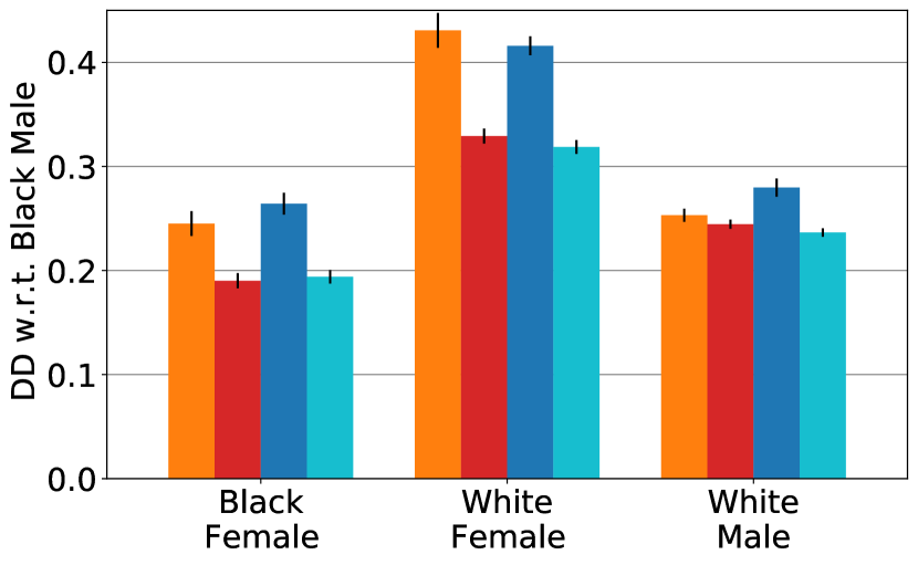
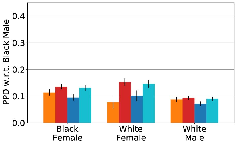
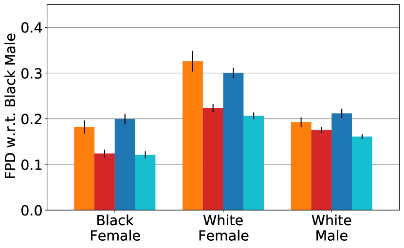
Measures. Since the non-discriminatory ground truth is unknown for these datasets, we use standard accuracy and demographic disparity to compare the learning algorithms. Demographic disparity measures disparate impact: $\text{DD}=|P(\hat{y}=1|z=0)-P(\hat{y}=1|z=1)|$ (Zafar et al., 2015; Salimi et al., 2019). While other measures have been proposed and used in the real-world context of applications (Larson et al., 2016), such as disparity in false positive rate ($\text{FPD}=|P(\hat{y}=1|y=0,z=0)-P(\hat{y}=1|y=0,z=1)|$) or positive predictive value ($\text{PPD}=|P(y=1|\hat{y}=1,z=0)-P(y=1|\hat{y}=1,z=1)|$), both of which we report, these and other measures derived from the confusion matrix are determined by accuracy and demographic disparity (Narayanan, 2018; Chouldechova, 2017; Kleinberg et al., 2017; Friedler et al., 2016). For the multiple protected attribute scenario, we report disparity for each combination of sex and race w.r.t. the largest and, across each measure, the most disadvantaged group in COMPAS, Black males.

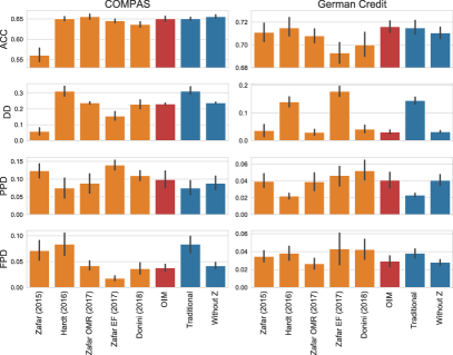
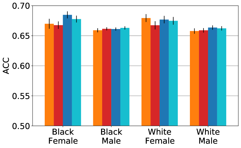
Results. We report the mean of the accuracy and disparities for the single-protected attribute scenarios in Figure 5. The results for the multi-protected attribute COMPAS scenario are reported in Figure 6.

For the German Credit data, the OIM achieves the lowest demographic disparity and the highest accuracy (the right panels of Figure 5). For the COMPAS data on one protected attribute it also achieves the top accuracy, while yielding medium demographic disparity. The method that achieves much lower demographic disparity than the OIM directly constrains disparate impact at the expense of drastically lower accuracy and higher other disparities (see ”Zafar” in the top left panel of Figure 5). The OIM also performs well in terms of false positive disparity and has medium performance for positive predictive disparity (the four bottom panels in Figure 5).

In the multiple protected attribute scenario, the OIM performed better than the traditional in demographic and false positive disparities, while maintaining high accuracy for each group (Figure 5 & 6). Therefore, the OIM addresses the substantial disparities in false positive rates by race reported in ProPublica’s analysis of COMPAS over all intersectional groups of race and sex (Larson et al., 2016). Even though the OIM resulted in marginally worse positive predictive disparity than the traditional method, as revealed in ProPublica’s analysis and our results, this disparity is minimal to begin with. The compared fair-learning method, “GerryFair” (Kearns et al., 2018), resulted in equal or more disparity than the OIM for DD and FPD (Figure 6). Adjusting its parameter $\gamma$’s value resulted either in increased accuracy with more disparity or vise-versa.

In both datasets and protected attribute scenarios, the OIM performs similarly to the traditional method that drops the protected attributes, “Without $Z$”; however, this method does not offer any protections, nor guarantees, against induced discrimination, as described in §4, and for the other datasets we studied it induces discrimination (see §6 and §7.2).

7.2. Concept shift information known

(a)

(b)

(c)

Figure 7. The expected cross-loss by hair-gender group (left plot) and the overall performance (right plot) of learning algorithms trained on the biased data following a discriminatory concept shift, except for the traditional trained on unbiased data (green bar). Marker style are shown in the photos on the left and have width of 10 pixels. Lower values are better. “Traditional” is ResNet-18.

Figure 8. Overall expected cross-loss and demographic disparity of learning algorithms as marking pixel size increases. Marker style as in 7a. Lower values are better. “Traditional” is ResNet-18.

Dataset. We focus on the CelebA dataset (Liu et al., 2015) commonly found in computer vision and deep learning literature. Here, the task is to classify the hair color of celebrities in photos, so the target labels are unlikely to be affected by any discrimination. In other words, the non-discriminatory $U$ is known and we can simulate discriminatory concept shift by swapping hair color labels to generate a discriminatory $Y$, which enable the measurements of cross-loss in real-world scenarios.

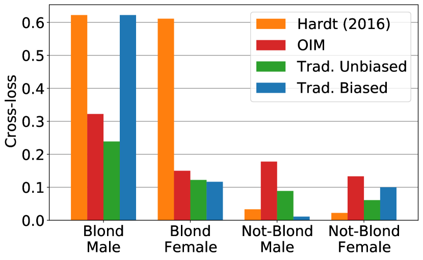
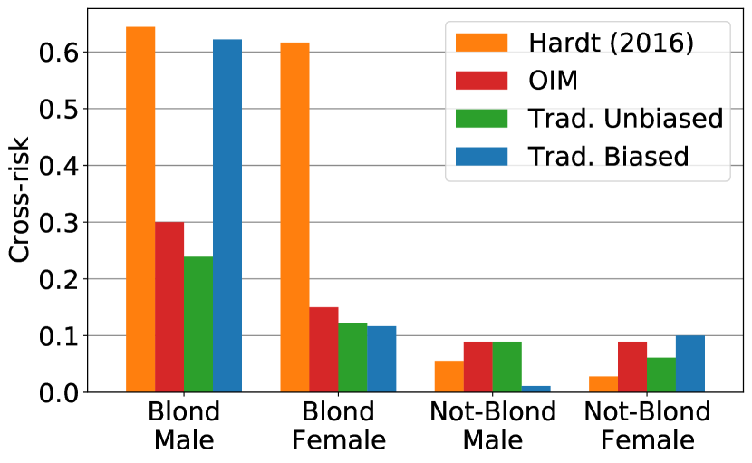
CelebA is composed of celebrity images, each with 40 attribute annotations. Each image is transformed to 128*128 pixels, constituting the features $\bm{X}$. We use the official train-val-test split from Liu et al. (2015) with blond ($y=1$) or not blond hair ($y=0$) as the target and binary gender as the protected attribute. To avoid sampling bias w.r.t. the hair-gender groups, we balance the dataset based on the smallest group (blond males). The balanced training and testing sets have 5,548 and 720 samples. To simulate a discriminatory concept shift, we swap the labels of 50% of blond males to not blond in the training data. We train the methods on this discriminatory data, except for the traditional method trained on the non-discriminatory data (green in Figure 7 & 8).

Models and training. As our base model architecture we use a Pytorch implementation of ResNet-18 (He et al., 2016). In addition to the OIM, only one of the evaluated learning methods’ implementation,  Hardt et al. (2016), can handle deep learning models, since both of them are post-processing methods. Therefore, all the methods train ResNet-18 on the images without annotations, then both fair learning methods use the gender annotations in their post-processing step. The OIM also requires the addition of the protected attribute to the feature set when training ResNet-18. To avoid any changes to the architecture, we encode gender in the images via special markings (e.g., 10 pixel wide green and blue boxes shown in Figure 7a). First, we train ResNet-18 on the photos with markings. Then, we estimate the optimal mixing distribution, $\pi^{*}$, on the training data. At the test time, we first compute the ResNet-18 predictions on the photos with either value of the gender mark, and then we average these predictions using the learned mixing distribution. Note that we do not use the ground-truth gender for making predictions in the test set, but rather the counterfactual values of the gender markings. Other methods train without these markings.

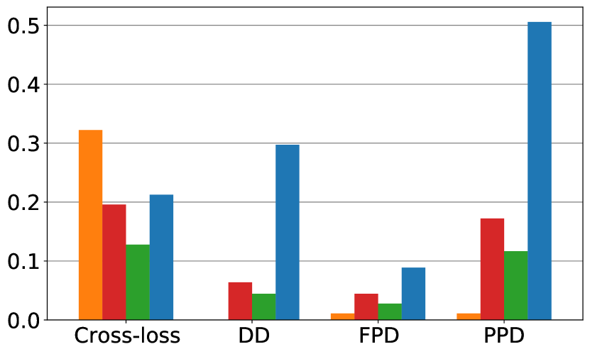
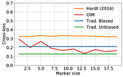
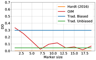
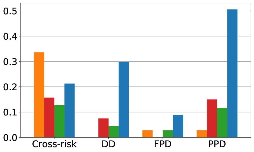
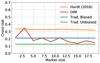
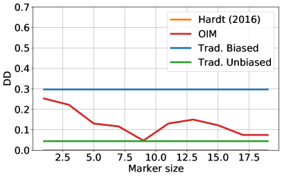
Results. We measure the expected cross-loss, demographic disparity (DD), false positive disparity (FPD), and positive predictive disparity (PPD). Despite training on the discriminatory data like the traditional biased method (blue in Figure 7), the OIM reduces the expected cross-loss and the disparities close to that of the traditional unbiased method (red and green in Figure 7). By contrast, when trained on discriminatory data, the traditional learning without $\bm{Z}$ (without markings) performs poorly both in terms of disparities and the cross-loss, especially for blond males whose label was swapped (blue in Figure 7). Without the gender encoding, the model uses visual features of the images, such as hair and face shape, as proxies for gender. The method by Hardt et al. (2016) results in the lowest DD and PPD (orange bars in Figure 7). However, it yields the highest expected cross-loss, in particular for the group with biased labels, i.e., blond males, and its female counterpart. In addition, this method tends to be further away (than the OIM) from the vanilla Resnet-18 training on the non-discriminatory data in terms of disparities. The presented OIM results use 10 pixel wide green boxes on the corners of images of females with same sized blue markings on male pictures (Figure 7a). The results for similar markings as Figure 7a are nearly the same (Appendix H). The expected cross-loss and the disparities of the OIM initially decrease monotonically with the width of the markings (Figure 8). At the width of about $10$ pixels this trend flattens, both in terms of expected cross-loss and disparities, suggesting that the markings are sufficiently large already for the model to use them. We note that, in real-world application domains where cross-loss cannot be measured, the size of markings can be established based on the disparity measures.

8. Conclusion

Discussion. Our results shed a new light on the problem of discrimination prevention in supervised learning. First, we propose a new objective for discrimination prevention in supervised learning seeking methods that are resilient to discriminatory dataset shifts. Dataset shifts clarify the dataset issues that can lead to discriminatory models. Different dataset shifts can be identified and tackled with different learning methods, so the remaining big question is whether these methods can be combined or are conflicting.

Second, we show that the optimal interventional mixtures do not produce reverse discrimination, nor induce discrimination. In the scenarios where training data is not discriminatory, the proposed learning method falls back to a traditional learning, and hence it is safer for general use than other approaches. While we do not provide resilience guarantees for discriminatory concept shifts with other perturbations than additive perturbations, to our knowledge this is the first study to provide such guarantees. Future research can study other dataset shifts to clarify the limits of this approach.

Third, we show that the proposed method is applicable to real-world settings with multiple protected groups and meets the explainability goal of removing their discriminatory impact, while remaining compatible with existing legal systems. The method provides a solution to the widely discussed issue of protected groups’ intersectionality and strikes a balance between protected groups, i.e., it does not correspond to affirmative actions advantageous to certain groups. The method overall is transparent and relatively easy to communicate to policymakers and courtroom officials.

Limitations. We studied a variety of datasets and models, finding support for our methods, but a wider set of scenarios could be considered. In future, discriminatory concept shifts could be measured via randomized human subject experiments or observational studies, and fair learning methods could be evaluated on resulting datasets and benchmarks. For instance, one could identify the groups of discriminating and fair members of hiring teams, as in our running Example, via population-level mixture models without identifying the individuals that belong to them (Grabowicz et al., 2018). Then, mixture components could be used to simulate realistic discriminatory and fair decisions. Such evaluation techniques would facilitate the comparisons and bolster the credibility of fair learning methods.

Appendix A: Proofs

(a) Logistic regression

(b) Linear regression

Figure 9. Resilience of learning algorithms to discrimination in a relevant attribute ($\tilde{X}_{1}$) for logistic regression and linear regression.

(a) Logistic regression

(b) Linear regression

Figure 10. Resilience of learning algorithms with $X_{2}$ missing during training to non-discriminatory perturbations (the leftmost column) and discriminatory perturbation (the remaining two columns), for logistic regression and linear regression.

Figure 11. Cumulative distribution function of per-dataset resilience of various learning algorithms ($\Omega_{a}$) divided by the resilience of the optimal interventional mixture ($\Omega_{\text{OIM}}$) for deep neural networks fitted to complex non-linear data generating models. The vertical red line is the CDF of the optimal interventional mixture applied to a neural network.

(a)

(b)

(c)

Figure 12. The cross-loss by hair-gender group (left plot) and the overall performance (right plot) of learning algorithms training on the perturbed data, except for one training on unbiased data (green bar). Marker style is as in (a) and size is 10 pixels. Lower values are better. “Traditional” is ResNet-18.

Figure 13. Overall cross-loss and demographic disparity of learning algorithms as marking pixel size increases. Marker style as in 12a. Lower values are better. “Traditional” is ResNet-18.

Proof of Proposition 1. From the definitions of consistent estimator and well-specified models, $\hat{y}(\bm{x},z)=\lim_{n\to\infty}\hat{y}_{n}(\bm{x},z)=f(\bm{x})+h(z)$, where $n$ is the size of the training dataset, $\hat{y}_{n}$ is a model trained on a given dataset. Note that $\nu$ is centered at zero, e.g., $\operatorname*{\mathbb{E}}[\nu]=0$ under $\ell^{2}$ or $\mathbb{M}[\nu]=0$ under $\ell^{1}$, where $\mathbb{M}$ stands for median; otherwise $f(\bm{x})$ can be redefined to center $\nu$. From the definition of the OIM and consistent estimator, $\hat{y}^{*}(\bm{x})=\lim_{n\to\infty}\hat{y}^{*}_{n}(\bm{x})=\operatorname*{\mathbb{E}}[\hat{y}(\bm{x},Z^{\prime})]=f(\bm{x})+C_{p}$. For $\ell^{2}$ loss, $C_{2}=\operatorname*{\mathbb{E}}[h(Z)+\nu]$, while for $\ell^{1}$ loss, $C_{1}=\mathbb{M}[h(Z)+\nu]$. For given datasets $D$ and $\tilde{D}$, the smaller the denominator in the definition of resilience, $\operatorname*{\mathbb{E}}_{D}\left[\ell\left(U,\hat{y}_{a}(\bm{X}|\tilde{D})\right)\right]$, the larger the resilience of the learning method. For the OIM, the denominator is $\operatorname*{\mathbb{E}}_{D}\left[\ell\left(U,\hat{y}^{*}(\bm{X})\right)\right]=\operatorname*{\mathbb{E}}[\ell(f(\bm{X})+\nu,f(\bm{X})+C_{p})]=\operatorname*{\mathbb{E}}[|\nu-C_{p}|^{p}]$. If $\operatorname*{\mathbb{E}}[h(Z)]=0$ under $\ell^{2}$ loss or $\mathbb{M}[h(Z)+\nu]=\mathbb{M}[\nu]=0$ under $\ell^{1}$ loss, then the OIM strictly maximizes the resilience, achieving $\operatorname*{\mathbb{E}}_{D}\left[\ell\left(U,\hat{y}^{*}(\bm{X})\right)\right]=0$ and $\Omega=1$. For an arbitrary model $\hat{y}(\bm{x})$, $\operatorname*{\mathbb{E}}_{D}\left[\ell\left(U,\hat{y}_{a}(\bm{x}|\tilde{D})\right)\right]=\operatorname*{\mathbb{E}}[\ell(f(\bm{X})+\nu,\hat{y}(\bm{x}))]=\operatorname*{\mathbb{E}}_{\bm{X}}\operatorname*{\mathbb{E}}_{\nu|\bm{X}}[|\nu+f_{1}(\bm{X})|^{p}]\geq\operatorname*{\mathbb{E}}_{\bm{X}}\operatorname*{\mathbb{E}}_{\nu|\bm{X}}[|\nu|^{p}]=\operatorname*{\mathbb{E}}_{D}\left[\ell\left(U,\hat{y}^{*}(\bm{X})\right)\right]|_{C_{p}=0}$, where $f_{1}(\bm{x})=f(\bm{x})-\hat{y}(\bm{x})$. Thus, the expected loss is minimized for $f_{1}(\bm{X})=0\iff\hat{y}(\bm{x})=f(\bm{x})$.

Proof of Corollary 1. Universal approximation theorems (Cybenko, 1989; Pinkus, 1999), which show that the loss of a universal approximator is bounded, $\sup_{\bm{x},z}\ell(g(\bm{x},z),\hat{y}_{\text{nn}}(\bm{x},z))<\epsilon$, for any positive $\epsilon$ and any function $g(\bm{x},z)$. In particular, $\ell^{p}(f(\bm{x})+h(z),\hat{y}_{\text{nn}}(\bm{x},z))<\epsilon$ and $<f(\bm{x})+h(z)-\epsilon^{p}<\hat{y}_{\text{nn}}(\bm{x},z)<f(\bm{x})+h(z)+\epsilon^{p}$. From the definition of the OIM, we get $<f(\bm{x})+C_{p}-\epsilon^{p}<\hat{y}_{\text{nn}}(\bm{x},z)<f(\bm{x})+C_{p}+\epsilon^{p}$ and $\ell^{p}(f(\bm{x})+h(z),f(\bm{x})+C_{p})<\epsilon$.

Proof of Proposition 2. Let the definitions and assumptions hold from the Proof of Proposition 1. From the definition of the MIM and consistent estimator, $\hat{y}_{\text{MIM}}(\bm{x})=\lim_{n\to\infty}\hat{y}^{*}_{n}(\bm{x})=\operatorname*{\mathbb{E}}_{\bm{Z}^{\prime}}[\hat{y}(\bm{x},Z^{\prime})]=f(\bm{x})+\operatorname*{\mathbb{E}}[h(Z)+\nu]$ for any loss. For given datasets $D$ and $\tilde{D}$, the smaller the denominator in the definition of resilience,
$\operatorname*{\mathbb{E}}_{D}\left[\ell\left(U,\hat{y}_{a}(\bm{X}|\tilde{D})\right)\right]$, the larger the resilience of the learning method. For the MIM, the denominator is $\operatorname*{\mathbb{E}}_{D}\left[\ell\left(U,\hat{y}_{\text{MIM}}(\bm{X})\right)\right]=\operatorname*{\mathbb{E}}[\ell(f(\bm{X})+\nu,f(\bm{X})+\operatorname*{\mathbb{E}}[h(Z)+\nu)]=\operatorname*{\mathbb{E}}[|\nu-\operatorname*{\mathbb{E}}[h(Z)]|^{p}]$. If $\operatorname*{\mathbb{E}}[h(Z)]=0$, then only under $\ell^{2}$ loss can the MIM strictly maximizes the resilience, achieving $\operatorname*{\mathbb{E}}_{D}\left[\ell\left(U,\hat{y}_{\text{MIM}}(\bm{X})\right)\right]=0$ and $\Omega=1$.

Appendix B: Data generation for random generalized linear models

We generate a synthetic set of $10\,000$ samples $\{(\bm{x},z)\}$ from a standard multivariate normal distribution with a random correlation matrix (Ghosh and Henderson, 2003). For simplicity, in our experiments we use two relevant features, that is $\bm{x}$ has two dimensions. The variable $z$ is converted to a binary value with the sign function. The coefficients $\bm{\alpha}$, $\bm{\tilde{\alpha}}$, and $\beta$ are drawn from $\text{Uniform}[-5,5]$, unless specified otherwise. We generate the non-discriminatory ground truth decisions, either as samples from 0-1 coin tosses, $u\sim\text{Bernoulli}[\operatorname*{\mathbb{E}}[U|\bm{x}]]$, or normal distribution with unit variance, $u\sim\text{Normal}[\operatorname*{\mathbb{E}}[U|\bm{x}],1]$.The resulting set of samples constitute the unperturbed evaluation dataset $D=\{(\bm{x},z,u)\}$. Finally, we sample the perturbed decisions, $y\sim\operatorname*{\textit{P}}(y|\bm{x},z)$, which contribute to the training dataset $\tilde{D}=\{(\bm{x},z,y)\}$.

Appendix C: Evaluation on a hiring scenario

Here, we present the results from a synthetic scenario proposed by (Lipton et al., 2018), modified slightly as follows. Using this example, we show how state-of-the-art learning algorithms addressing discrimination induce it even when the training data is non-discriminatory.

To this end, we sample 1000 observations from the data-generating process below:

$$z_{i}\sim\text{Bernoulli}[0.5]$$

$$\text{hair\_length}_{i}|z_{i}=0\sim 35*\text{Beta[2, 2]}$$

$$\text{hair\_length}_{i}|z_{i}=1\sim 35*\text{Beta[2, 7]}$$

$$\text{work\_exp}_{i}|z_{i}=0\sim\text{Poisson}[25]-\text{Normal}[20,\sigma=0.2]$$

$$\text{work\_exp}_{i}|z_{i}=1\sim\begin{cases}\text{Normal}[10,\sigma=2]&\text{w/ prob 0.2}\\ \text{Normal}[15,\sigma=2]&\text{w/ prob 0.8}\end{cases}$$

$$p_{i}=f(-25.5+2.5*\text{work\_exp})\text{ where }f(x)=\frac{1}{1+e^{-x}}$$

$$y_{i}|\text{work\_exp}\sim\text{Bernoulli}[p_{i}]$$

This synthetic data represents the historical hiring process where the protected attribute is a candidate’s gender, $z$. The data has the following properties: i) the hiring decision has been made based on the work experience only, thus, it is non-discriminatory data; ii) since women on average have less work experience than men, men have been hired at higher rate than women historically; and iii) women tend to have longer hair than men. Therefore, a model that uses hair length in its decision-making can induce indirect discrimination. Additionally, we introduced modifications to this synthetic data with respect to the original scenario (Lipton et al., 2018). The work experience of male candidates now follows a bi-modal distribution (i.e., a mixture of two normal distributions) with one peak at 10 and another at 15. We trained a method for discrimination prevention (Zafar et al., 2017b) under three different fairness constraints: equalized misclassification rate, false positive rate (FPR), false negative rate (FNR). We also trained a model while simultaneously optimizing both FPR and FNR; however, the learned model returned trivial predictions where all candidates are rejected. The relative utility of the various methods is low compared with the OIM.

Method	$\operatorname*{\mathbb{E}}[R_{\text{perf}}/R]$
OIM	1.000
Zafar et al. (2017c)	0.997
Zafar et al. (2017b) with FNR	0.838
Zafar et al. (2017b) with Missclass.	0.777
Donini et al. (2018)	0.634
Zafar et al. (2017b) with FPR	0.570
Hardt et al. (2016)	0.328
Zafar et al. (2015)	0.179

Table 1. Relative utility of various fairness models (Hardt et al., 2016; Donini et al., 2018; Zafar et al., 2015, 2017b; Zafar et al., 2017c) trained with the synthetic data

Appendix D: Random generalized linear models

We check whether the results from §6 hold over various parameters of data generating processes. For each learning algorithm, the procedure of data generation and training is repeated $1000$ times, each time with a different correlation matrix $\Sigma$ and parameters $\alpha$, $\tilde{\alpha}$, $\beta$ (additional details in Appendix B). We report mean resilience of each learning algorithm, averaged over randomly generated datasets (Figure 14).

When the learning algorithms preventing discrimination are applied to non-discriminatory data, they should fall back to a traditional learning algorithm to avoid biases in inference and yield perfect resilience. For logistic regression, only two algorithms achieve this for all datasets: the method based on envy-freeness (“Zafar EF” in the upper leftmost Figure 14) (Zafar et al., 2017c) and our OIM (the red bar in the upper leftmost Figure 14). The OIM is also more resilient to directly discriminatory perturbations than other supervised methods aiming to prevent discrimination for logistic regression (the middle and rightmost panels in upper Figure 14). The second best method is traditional learning (with or without the protected attribute; blue bars in upper Figure 14), and third is the game-theoretic method based on envy-freeness(“Zafar EF” in upper Figure 14). However, these two methods allow direct discrimination via $Z$ (middle upper Figure 14).

The difference between the OIM and traditional learning is small for logistic regression (upper Figure 14), but it is large for linear regression (lower Figure 14). For the linear regression model, the proposed method achieves maximal resilience to directly discriminatory perturbations (lower Figure 14). Here the difference in resilience between the OIM and other methods is significantly greater than that for logistic regression (upper Figure 14).

(a) Logistic regression

(b) Linear regression

Figure 14. Resilience of various learning algorithms for logistic regression (upper) averaged over datasets. Error bars correspond to $95\%$ confidence intervals of the expectation, obtained via bootstrapping.

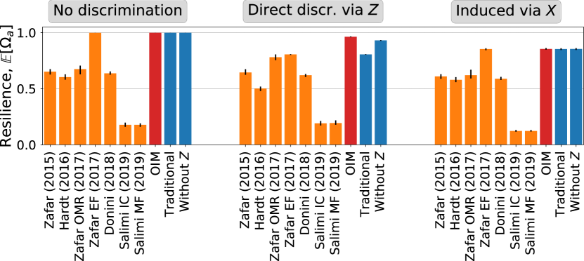
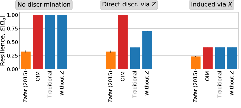
Appendix E: Features affected by direct discrimination

Apart from the perturbations of the output variable, $U$, the perturbed dataset, $\tilde{D}$ could also include the perturbations of some of the relevant attribute $X_{1}$. We refer to such relevant attribute as $\tilde{X}_{1}$. From the perspective of decisions $Y$, such perturbations result in indirect discrimination, because they impact $Y$ indirectly through $\bm{X}$. For instance, Jim Crow laws required literacy to decide whether an individual has a voting right, while ethnic minorities had systematically limited access to education (Klarman, 2006). If some $\tilde{X}_{1}$ is the outcome of human decisions and is affected by direct discrimination, then we could and should apply the same reasoning and methods as we do to $Y$, i.e., we shall construct a respective model for $\tilde{X}_{1}$, in which this variable is treated as an output variable. Then, one can obtain an estimator of $X_{1}$ based on $\tilde{X}_{1}$ by applying the OIM. The computed OIM of $X_{1}$ can be used to also obtain an estimator of $U$ based on $Y$. We apply this procedure within our evaluation framework by modeling a perturbation of $X_{1}$ in the same manner as of $U$. We measure the resilience of the learning algorithms to this perturbation finding that the OIM prevents direct discrimination in $\bm{X}$ and as a consequence in $U$ (Figure 9), under a linear model of $\bm{X}$ and either a logistic or linear model of $Y$.

Appendix F: Missing features.

In real-world settings, attributes are often unknown or their measurements are unavailable. We model this scenario by removing $X_{2}$ from the training dataset $\tilde{D}$, while keeping it unchanged in $D$. Then, we measure the resilience of learning algorithms to the non-discriminatory and discriminatory perturbation.

When $X_{2}$ is missing, we obtain nearly identical relative resilience results as before. The OIM is more resilient to direct and induced discriminatory perturbations than the other supervised methods aiming to prevent discrimination (Figure 10). For logistic regression, the game-theoretic method based on envy-freeness, “Zafar EF” (the upper middle and rightmost panels in Figure 10) has only slightly worse performance for direct discrimination, and the same or slightly better performance when there is no discrimination or when there is induced discrimination. Since these methods are missing one of the attributes required to model the data generating process, their predictions are significantly worse and resilience is considerably less than in the case where all attributes are available for training. However, except for “Zafar EF”, the resilience remains similar in ranking between methods to the scenario where all attributes are available.

Appendix G: Non-linear models.

In addition to missing features, real-world data may be generated by complex non-linear processes that cannot be fit using simple models like logistic regression. To simulate this scenario, we introduce a non-linearity in $f(\bm{x})$. Here we present the results for $f(\bm{x})=\alpha_{1}x_{1}x_{2}$, but we obtain the same qualitative results for other functional forms, such as $f(\bm{x})=\alpha_{1}\exp(\alpha_{2}x_{1}x_{2})$ and $f(\bm{x})=\alpha_{1}\sin(\alpha_{2}x_{1}x_{2})$, where parameters $\alpha_{i}$ are random as in Appendix B. To learn these more complex models, we apply the OIM to deep neural networks (OIM-NN). We utilize a relatively simple architecture: three-fully connected hidden layers with the ReLU activation function and a sigmoid output layer. The hyperparameters are tuned to optimize accuracy as usual. Most other methods do not have implementations for deep learning models, so we cannot evaluate them, except for the traditional learning and the post-processing method based on equalized odds (Hardt et al., 2016).

To provide more details, we report the cumulative distribution function of per-dataset resilience of each learning algorithm, $\Omega_{a}$, divided by the resilience of the OIM-NN, $\Omega_{\text{OIM}}$, for classification (Figure 11). The deep learning models are more resilient to data perturbations than their logistic regression counterparts for nearly all datasets (“NN” versus “LR” in Figure 11), since neural networks are better suited to approximate the non-linear data. Most importantly, the OIM-NN tends to outperform all other methods. When compared to the traditional deep learning without $Z$, the OIM-NN is more resilient to directly discriminatory perturbations of data for 80% of datasets (blue dashed line in the middle Figure 11).

Appendix H: The choice of image markings

We show that the results between an alternative box marking style (Figure 12a) and the box marking style presented in the main text (Figure 7 & 8) are nearly identical. Furthermore with this alternative marking style, we show how the effect of the marker size affects the performance of the OIM as in the main text (Figure 13).

References

- (1)
- Altman (2016) Andrew Altman. 2016. Discrimination. In The Stanford Encyclopedia of Philosophy (2016 ed.), Edward N Zalta (Ed.). Metaphysics Research Lab, Stanford University.
- Barocas et al. (2019) Solon Barocas, Moritz Hardt, and Arvind Narayanan. 2019. Fairness and Machine Learning: Limitations and Opportunities. fairmlbook.org. http://www.fairmlbook.org.
- Bartlett et al. (2019) Robert Bartlett, Adair Morse, Richard Stanton, and Nancy Wallace. 2019. Consumer-Lending Discrimination in the FinTech Era. Technical Report. National Bureau of Economic Research, Cambridge, MA. 1–51 pages. https://doi.org/10.3386/w25943
- Bertrand and Mullainathan (2003) Marianne Bertrand and Sendhil Mullainathan. 2003. Are Emily and Greg More Employable than Lakisha and Jamal? A Field Experiment on Labor Market Discrimination. Technical Report. National Bureau of Economic Research, Cambridge, MA. https://doi.org/10.3386/w9873
- Bickel et al. (1975) P. J. Bickel, E. A. Hammel, and J. W. O’Connell. 1975. Sex Bias in Graduate Admissions: Data from Berkeley. Science 187, 4175 (feb 1975), 398–404. https://doi.org/10.1126/science.187.4175.398
- Blueprint for an AI Bill of Rights (2022) Blueprint for an AI Bill of Rights. 2022. https://www.whitehouse.gov/ostp/ai-bill-of-rights/
- Chiappa (2019) Silvia Chiappa. 2019. Path-Specific Counterfactual Fairness. Proceedings of the AAAI Conference on Artificial Intelligence 33 (jul 2019), 7801–7808. https://doi.org/10.1609/aaai.v33i01.33017801
- Chouldechova (2017) Alexandra Chouldechova. 2017. Fair Prediction with Disparate Impact: A Study of Bias in Recidivism Prediction Instruments. Big Data 5, 2 (jun 2017), 153–163. https://doi.org/10.1089/big.2016.0047 arXiv:1703.00056
- Crenshaw (2017) Kimberle W. Crenshaw. 2017. ”On Intersectionality: Essential Writings. Faculty Books. https://scholarship.law.columbia.edu/books/255.
- Cybenko (1989) G. Cybenko. 1989. Approximation by superpositions of a sigmoidal function. Mathematics of Control, Signals, and Systems 2, 4 (dec 1989), 303–314. https://doi.org/10.1007/BF02551274
- Datta et al. (2016) Anupam Datta, Shayak Sen, and Yair Zick. 2016. Algorithmic Transparency via Quantitative Input Influence: Theory and Experiments with Learning Systems. Proceedings - 2016 IEEE Symposium on Security and Privacy, SP 2016 (2016), 598–617. https://doi.org/10.1109/SP.2016.42
- Diamond and Boyd (2016) Steven Diamond and Stephen Boyd. 2016. CVXPY: A Python-embedded modeling language for convex optimization. Journal of Machine Learning Research 17 (2016), 1–5.
- Donini et al. (2018) Michele Donini, Luca Oneto, Shai Ben-David, John Shawe-Taylor, and Massimiliano Pontil. 2018. Empirical risk minimization under fairness constraints. Advances in Neural Information Processing Systems 2018-Decem, NeurIPS (2018), 2791–2801.
- Dua and Graff (2017) Dheeru Dua and Casey Graff. 2017. UCI Machine Learning Repository. http://archive.ics.uci.edu/ml
- Feldman et al. (2014) Michael Feldman, Sorelle Friedler, John Moeller, Carlos Scheidegger, and Suresh Venkatasubramanian. 2014. Certifying and removing disparate impact. (2014), 259–268. https://doi.org/10.1145/2783258.2783311 arXiv:1412.3756
- Fish et al. (2016) Benjamin Fish, Jeremy Kun, and Ádám D. Lelkes. 2016. A confidence-based approach for balancing fairness and accuracy. 16th SIAM International Conference on Data Mining 2016, SDM 2016 (2016), 144–152. https://doi.org/10.1137/1.9781611974348.17 arXiv:1601.05764
- Friedler et al. (2016) Sorelle A. Friedler, Carlos Scheidegger, and Suresh Venkatasubramanian. 2016. On the (im)possibility of fairness. (2016). arXiv:1609.07236 http://arxiv.org/abs/1609.07236
- Ghosh and Henderson (2003) Soumyadip Ghosh and Shane G Henderson. 2003. Behavior of the NORTA method for correlated random vector generation as the dimension increases. ACM Transactions on Modeling and Computer Simulation 13, 3 (jul 2003), 276–294. https://doi.org/10.1145/937332.937336
- Grabowicz et al. (2022) Przemyslaw A. Grabowicz, Nicholas Perello, and Aarshee Mishra. 2022. Marrying Fairness and Explainability in Supervised Learning. In 2022 ACM Conference on Fairness, Accountability, and Transparency (Seoul, Republic of Korea) (FAccT ’22). Association for Computing Machinery, New York, NY, USA, 1905–1916. https://doi.org/10.1145/3531146.3533236
- Grabowicz et al. (2018) Przemyslaw A Grabowicz, Francisco Romero-Ferrero, Theo Lins, Fabrício Benevenuto, Krishna P Gummadi, and Gonzalo G De Polavieja. 2018. Experimental Evidence for Bayesian Social Influence. Submission to PNAS (2018).
- Halpern et al. (2018) Naama Halpern, Yael Goldberg, Luna Kadouri, Morasha Duvdevani, Tamar Hamburger, Tamar Peretz, Ayala Hubert, Joy Buolamwini, and Timnit Gebru. 2018. Gender Shades: Intersectional Accuracy Disparities in Commercial Gender Classification. In Proceedings of Machine Learning Research (Proceedings of Machine Learning Research, Vol. 81), Sorelle A Friedler and Christo Wilson (Eds.). PMLR, New York, NY, USA, 77–91. http://proceedings.mlr.press/v81/buolamwini18a.htmlhttps://www.dovepress.com/clinical-course-and-outcome-of-patients-with-high-level-microsatellite-peer-reviewed-article-OTT
- Hardt et al. (2016) Moritz Hardt, Eric Price, and Nathan Srebro. 2016. Equality of Opportunity in Supervised Learning. In Advances in Neural Information Processing Systems, D D Lee, M Sugiyama, U V Luxburg, I Guyon, and R Garnett (Eds.). Curran Associates, Inc., 3315–3323. https://doi.org/10.1109/ICCV.2015.169 arXiv:1610.02413
- He et al. (2016) Kaiming He, X. Zhang, Shaoqing Ren, and Jian Sun. 2016. Deep Residual Learning for Image Recognition. 2016 IEEE Conference on Computer Vision and Pattern Recognition (CVPR) (2016), 770–778.
- Hernandez (2009) Jesus Hernandez. 2009. Redlining revisited: mortgage lending patterns in Sacramento 1930–2004. International Journal of Urban and Regional Research 33, 2 (2009), 291–313.
- Janzing et al. (2019) Dominik Janzing, Lenon Minorics, and Patrick Blöbaum. 2019. Feature relevance quantification in explainable AI: A causal problem. 2015 (oct 2019). arXiv:1910.13413 http://arxiv.org/abs/1910.13413
- Kearns et al. (2018) Michael Kearns, Seth Neel, Aaron Roth, and Zhiwei Steven Wu. 2018. Preventing Fairness Gerrymandering: Auditing and Learning for Subgroup Fairness. In Proceedings of the 35th International Conference on Machine Learning (Proceedings of Machine Learning Research, Vol. 80), Jennifer Dy and Andreas Krause (Eds.). PMLR, 2564–2572. https://proceedings.mlr.press/v80/kearns18a.html
- Kilbertus et al. (2017) Niki Kilbertus, Mateo Rojas Carulla, Giambattista Parascandolo, Moritz Hardt, Dominik Janzing, and Bernhard Schölkopf. 2017. Avoiding Discrimination through Causal Reasoning. In Advances in Neural Information Processing Systems 30. Curran Associates, Inc., 656–666. arXiv:1706.02744 http://arxiv.org/abs/1706.02744http://papers.nips.cc/paper/6668-avoiding-discrimination-through-causal-reasoning.pdf
- Klarman (2006) Michael J Klarman. 2006. From Jim Crow to civil rights: The Supreme Court and the struggle for racial equality. Oxford University Press.
- Kleinberg et al. (2017) Jon Kleinberg, Sendhil Mullainathan, and Manish Raghavan. 2017. Inherent Trade-Offs in the Fair Determination of Risk Scores. In Proceedings of Innovations in Theoretical Computer Science (ITCS). https://doi.org/10.1111/j.1740-9713.2017.01012.x arXiv:1609.05807
- Koh et al. (2020) Pang Wei Koh, Shiori Sagawa, Henrik Marklund, Sang Michael Xie, Marvin Zhang, Akshay Balsubramani, Weihua Hu, Michihiro Yasunaga, Richard Lanas Phillips, Sara Beery, Jure Leskovec, Anshul Kundaje, Emma Pierson, Sergey Levine, Chelsea Finn, and Percy Liang. 2020. WILDS: A Benchmark of in-the-Wild Distribution Shifts. (2020), 1–87. arXiv:2012.07421 http://arxiv.org/abs/2012.07421
- Kusner et al. (2017) Matt J. Kusner, Joshua R. Loftus, Chris Russell, and Ricardo Silva. 2017. Counterfactual Fairness. In Advances in Neural Information Processing Systems 30, I Guyon, U V Luxburg, S Bengio, H Wallach, R Fergus, S Vishwanathan, and R Garnett (Eds.). Curran Associates, Inc., 4066–4076. arXiv:1703.06856 http://arxiv.org/abs/1703.06856http://papers.nips.cc/paper/6995-counterfactual-fairness.pdf
- Larson et al. (2016) Jeff Larson, Surya Mattu, Lauren Kirchner, and Julia Angwin. 2016. How We Analyzed the COMPAS Recidivism Algorithm. Pro Publica (2016). https://www.propublica.org/article/how-we-analyzed-the-compas-recidivism-algorithm
- Lippert-Rasmussen (2012) Kasper Lippert-Rasmussen. 2012. The Badness of Discrimination. 9, 2 (2012), 167–185. https://doi.org/10.1007/sl0677-006-9014-x
- Lipton et al. (2018) Zachary C. Lipton, Alexandra Chouldechova, and Julian McAuley. 2018. Does mitigating ML’s impact disparity require treatment disparity? Advances in Neural Information Processing Systems 2018-Decem, ML (2018), 8125–8135.
- Lipton and Steinhardt (2019) Zachary C. Lipton and Jacob Steinhardt. 2019. Troubling trends in machine-learning scholarship. Queue 17, 1 (2019), 1–15. https://doi.org/10.1145/3317287.3328534 arXiv:1807.03341
- Liu et al. (2015) Ziwei Liu, Ping Luo, Xiaogang Wang, and Xiaoou Tang. 2015. Deep Learning Face Attributes in the Wild. In Proceedings of International Conference on Computer Vision (ICCV).
- Lu et al. (2019) Jie Lu, Anjin Liu, Fan Dong, Feng Gu, Joao Gama, and Guangquan Zhang. 2019. Learning under Concept Drift: A Review. IEEE Transactions on Knowledge and Data Engineering 31, 12 (2019), 2346–2363. https://doi.org/10.1109/TKDE.2018.2876857 arXiv:2004.05785
- Lundberg and Lee (2017) Scott M Lundberg and Su-In Lee. 2017. A Unified Approach to Interpreting Model Predictions. In Advances in Neural Information Processing Systems 30, I. Guyon, U. V. Luxburg, S. Bengio, H. Wallach, R. Fergus, S. Vishwanathan, and R. Garnett (Eds.). Curran Associates, Inc., 4765–4774. http://papers.nips.cc/paper/7062-a-unified-approach-to-interpreting-model-predictions.pdf
- Marx et al. (2019) Charles T. Marx, Richard Lanas Phillips, Sorelle A. Friedler, Carlos Scheidegger, and Suresh Venkatasubramanian. 2019. Disentangling influence: Using disentangled representations to audit model predictions. Advances in Neural Information Processing Systems 32 (2019). arXiv:1906.08652
- Moreno-Torres et al. (2012) Jose G. Moreno-Torres, Troy Raeder, Rocío Alaiz-Rodríguez, Nitesh V. Chawla, and Francisco Herrera. 2012. A unifying view on dataset shift in classification. Pattern Recognition 45, 1 (2012), 521–530. https://doi.org/10.1016/j.patcog.2011.06.019
- Nabi et al. (2019) Razieh Nabi, Daniel Malinsky, and Ilya Shpitser. 2019. Learning Optimal Fair Policies. In Proceedings of the 36th International Conference on Machine Learning. PMLR 97:4674–4682. arXiv:1809.02244 http://arxiv.org/abs/1809.02244
- Narayanan (2018) Arvind Narayanan. 2018. Tutorial: 21 fairness definitions and their politics. https://www.youtube.com/watch?v=jIXIuYdnyyk
- on Further Advancing Racial Equity and for Underserved Communities Through The Federal Government (2023) Executive Order on Further Advancing Racial Equity and Support for Underserved Communities Through The Federal Government. 2023. https://www.whitehouse.gov/briefing-room/presidential-actions/2023/02/16/executive-order-on-further-advancing-racial-equity-and-support-for-underserved-communities-through-the-federal-government/
- Pearl (2009) Judea Pearl. 2009. Causality: Models, Reasoning and Inference (2nd ed.). Cambridge University Press.
- Pearl et al. (2016) Judea Pearl, Madelyn Glymour, and Nicolas P. Jewell. 2016. Causal Inference in Statistics: A Primer.
- Pedreshi et al. (2008) Dino Pedreshi, Salvatore Ruggieri, and Franco Turini. 2008. Discrimination-aware data mining. In Proceeding of the 14th ACM SIGKDD international conference on Knowledge discovery and data mining - KDD 08. ACM Press, New York, New York, USA, 560. https://doi.org/10.1145/1401890.1401959
- Pinkus (1999) Allan Pinkus. 1999. Approximation theory of the MLP model in neural networks. Acta Numerica 8 (1999), 143–195. https://doi.org/10.1017/S0962492900002919
- Pleiss et al. (2017) Geoff Pleiss, Manish Raghavan, Felix Wu, Jon Kleinberg, and Kilian Q. Weinberger. 2017. On Fairness and Calibration. In Advances in Neural Information Processing Systems 30, I Guyon, U V Luxburg, S Bengio, H Wallach, R Fergus, S Vishwanathan, and R Garnett (Eds.). Curran Associates, Inc., 5680–5689. arXiv:1709.02012 http://arxiv.org/abs/1709.02012http://papers.nips.cc/paper/7151-on-fairness-and-calibration.pdf
- Ricci v. DeStefano 557 U.S. 557, Docket No. 07-1428 (2009) Ricci v. DeStefano 557 U.S. 557, Docket No. 07-1428. 2009. Supreme Court of the United States.
- Rovner (2018) Joshua Rovner. 2018. Report to the United Nations on Racial Disparities in the U.S. Criminal Justice System. https://www.sentencingproject.org/reports/report-to-the-united-nations-on-racial-disparities-in-the-u-s-criminal-justice-system/
- Sagawa et al. (2020) Shiori Sagawa, Aditi Raghunathan, Pang Wei Koh, and Percy Liang. 2020. An Investigation of Why Overparameterization Exacerbates Spurious Correlations. In ICML’20. arXiv:2005.04345 http://arxiv.org/abs/2005.04345
- Salimi et al. (2019) Babak Salimi, Luke Rodriguez, Bill Howe, and Dan Suciu. 2019. Capuchin: Causal Database Repair for Algorithmic Fairness. (feb 2019). arXiv:1902.08283 http://arxiv.org/abs/1902.08283
- The Fair Housing Act (1968) The Fair Housing Act. 1968. 42 U.S.C.A., 3601-3631.
- Title VII of the Civil Rights Act (1964) Title VII of the Civil Rights Act. 1964. 7, 42 U.S.C., 2000e et seq.
- Ture et al. (1968) Kwame Ture, Charles V Hamilton, and Stokely Carmichael. 1968. Black power: The politics of liberation in America: With new afterwords by the authors. Vintage Books.
- Turner and Skidmore (1999) Margery Austin Turner and Felicity Skidmore. 1999. Mortgage Lending Discrimination : A Review of Existing Evidence Lending Discrimination : A Review of existing Evidence. In The Urban Institute. 1–176.
- Wachter (2019) Sandra Wachter. 2019. Affinity Profiling and Discrimination by Association in Online Behavioural Advertising. SSRN Electronic Journal (2019), 1–74. https://doi.org/10.2139/ssrn.3388639
- Wang et al. (2022) Angelina Wang, Vikram V Ramaswamy, and Olga Russakovsky. 2022. Towards Intersectionality in Machine Learning: Including More Identities, Handling Underrepresentation, and Performing Evaluation. In 2022 ACM Conference on Fairness, Accountability, and Transparency (Seoul, Republic of Korea) (FAccT ’22). Association for Computing Machinery, New York, NY, USA, 336–349. https://doi.org/10.1145/3531146.3533101
- Widmer and Kubat (1996) Gerhard Widmer and Miroslav Kubat. 1996. Learning in the presence of concept drift and hidden contexts. Machine Learning 23, 1 (1996), 69–101. https://doi.org/10.1023/A:1018046501280
- Woodworth et al. (2017) Blake Woodworth, Suriya Gunasekar, Mesrob I. Ohannessian, and Nathan Srebro. 2017. Learning Non-Discriminatory Predictors. 1 (2017). arXiv:1702.06081 http://arxiv.org/abs/1702.06081
- Wu et al. (2019) Yongkai Wu, Lu Zhang, Xintao Wu, and Hanghang Tong. 2019. PC-Fairness: A unified framework for measuring causality-based fairness. Advances in Neural Information Processing Systems 32, NeurIPS (2019). arXiv:1910.12586
- Zafar et al. (2017a) Muhammad Bilal Zafar, Isabel Valera, Manuel Gomez Rodriguez, and Krishna P. Gummadi. 2017a. Fairness Beyond Disparate Treatment & Disparate Impact: Learning Classification without Disparate Mistreatment. In Proceedings of the 26th International Conference on World Wide Web - WWW ’17. ACM Press, New York, New York, USA, 1171–1180. https://doi.org/10.1145/3038912.3052660 arXiv:1610.08452
- Zafar et al. (2015) Muhammad Bilal Zafar, Isabel Valera, Manuel Gomez Rodriguez, and Krishna P Gummadi. 2015. Fairness Constraints: Mechanisms for Fair Classification. Fairness, Accountability, and Transparency in Machine Learning (jul 2015). arXiv:1507.05259 http://arxiv.org/abs/1507.05259
- Zafar et al. (2017b) Muhammad Bilal Zafar, Isabel Valera, Manuel Gomez Rodriguez, and Krishna P Gummadi. 2017b. Fairness Constraints: Mechanisms for Fair Classification. Artificial Intelligence and Statistics 54 (2017). arXiv:1507.05259 https://arxiv.org/abs/1507.05259
- Zafar et al. (2017c) Muhammad Bilal Zafar, Isabel Valera, Manuel Gomez Rodriguez, Krishna P. Gummadi, and Adrian Weller. 2017c. From Parity to Preference-based Notions of Fairness in Classification. In Advances in Neural Information Processing Systems 30, I Guyon, U V Luxburg, S Bengio, H Wallach, R Fergus, S Vishwanathan, and R Garnett (Eds.). Curran Associates, Inc., 229–239. arXiv:1707.00010 http://arxiv.org/abs/1707.00010http://papers.nips.cc/paper/6627-from-parity-to-preference-based-notions-of-fairness-in-classification.pdf
- Zenou and Boccard (2000) Yves Zenou and Nicolas Boccard. 2000. Racial discrimination and redlining in cities. Journal of Urban economics 48, 2 (2000), 260–285.
- Zhang and Bareinboim (2018) Junzhe Zhang and Elias Bareinboim. 2018. Fairness in Decision-Making – The Causal Explanation Formula. AAAI (2018), 2037–2045. https://www.aaai.org/ocs/index.php/AAAI/AAAI18/paper/view/16949
- Zhang et al. (2017) Lu Zhang, Yongkai Wu, and Xintao Wu. 2017. A causal framework for discovering and removing direct and indirect discrimination. IJCAI International Joint Conference on Artificial Intelligence 0 (2017), 3929–3935. https://doi.org/10.24963/ijcai.2017/549 arXiv:1611.07509