An Extreme Metastable Model for Quantum Measurement

Abstract.

Quantum experiments are observed as probability density functions. We often encounter multi-peaked densities which we model in this paper by a metastable dynamical system. The dynamics can be regarded in a thought experiment where a mouse is in either one of two disjoint traps which possess little outlets. The mouse spends most of its time in one or the other trap, and once in awhile makes its way to the other trap. Hence, a bi-peaked density function. When the experiment is observed - such as a light shone on the traps - the mouse stays in one trap. This measurement process results in a single peaked density that, we prove, can be modelled by the metastable process selecting an extreme density function, which is single peaked.

Highlights:

1. Many quantum mechanical processes display a multi-peaked density function.

2. We model the underlying dynamics by a metastable dynamical system based on a piecewise expanding map.

3. A measurement on the process results in a single peaked density function, which we prove is an extreme metastable system.

Department of Mathematics and Statistics, Concordia University, 1455 de Maisonneuve Blvd. West, Montreal, Quebec H3G 1M8, Canada

and

Department of Mathematics, Honghe University, Mengzi, Yunnan 661100, China

E-mails: abraham.boyarsky@concordia.ca, pawel.gora@concordia.ca, zhenyangemail@gmail.com.

1. Introduction

The behavior of quantum systems is governed by the Schrodinger‘s Wave Equation. The complex-valued solutions of these equations are called wave functions. When squared, the wave equation describes the probability of a quantum particle being found in various locations of the state space. Quantum particles have no fixed location. Their existence is spread probabilistically across the domain of the wave function. However, when a macro measurement is made there is an instantaneous and dramatic change: all random effects vanish and real properties immediately appear. Quantum theory does not explain why and what happens as probability turns into certainty. This transition is called collapse of the wavefunction and the mysterious effect is referred to as the measurement problem.

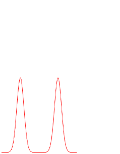
Figure 1. Probability density function with two narrow peaks

A common way of portraying the measurement problem is to display the probability density function (pdf) of finding a quantum particle. In the quantum case it is a pdf $f\$ with two narrow peaks [3, page 31]. When a measurement is made one or other of the two peaks vanishes and the quantum particle is localized to the remaining single peak region of the state space. There are various explanations for this effect: for example, decoherence and continuous spontaneous localization, but neither are completely satisfactory.

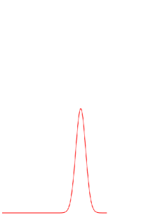
Figure 2. Probability density function $f_{0}$ with one narrow peak

In this note we will model the measurement problem by using a deterministic metastable system. First, we refer to the following thought experiment: a mouse is moving about in a set $A$ which has a small escape hatch. The mouse spends most of its time in $A$, but now and again it escapes and makes its way to a set $B$ where it behaves in the same way as in $A$. To locate the mouse a light is shone on the setup. The process of shining light is a macro measurement; it frightens the mouse and it no longer ventures out of the set it is in at the time of measurement.

In section 2 we describe a general discrete time metastable system that models the above mouse trap experiment. At the outset we assume that a map $T$ satisfies the conditions of [4] that are sufficient for for its deterministic perturbation $T_{\varepsilon}$ to be metastable as well as generating the pdf $f$  described above. Note that our starting point is not the wave function $\psi$ but rather the two peaked pdf $f$ which stems from a wave function $\psi$. We do not attempt to relate $T$ to $\psi$, although both generate $f$ but in completely different ways.

Let $A$ and $B$ be two disjoint sets of the state space. $T$ is assumed to have an absolutely continuous invariant measure (acim) $\mu$ (not ergodic) on $A\cup B.$ Now we assume that there are two mutually singular ergodic acims $\mu_{A}$ and $\mu_{B},\$ on $A$ and $B,$ respectively, where $\mu_{A}$ and $\mu_{B}$ have probability density functions (pdf) $f_{A}$ and $f_{B}$. Rather than refer back to the wave functions that generate these pdfs, we construct a piecewise smooth expanding map $T$ that has invariant densities $f_{A}$ and $f_{B}.$To model the motion of a quantum particle which, like the mouse in the thought experiment, can be found in either $A$ or $B,$ we define a metastable map $T_{\varepsilon}$ which is an $\varepsilon$ determinsitic perturbation of $T.\ T_{\varepsilon\text{ }}$causes $A$ and $B$ to forfeit their invariance and creates a single acim $\mu_{\epsilon}$ on $A\cup B.$ The measure $\mu_{\epsilon}$ has a pdf $f_{\varepsilon}$ which converges to a convex combination of $f_{A}$ and $f_{B}$ as $\varepsilon\rightarrow 0$. The set of densities $\mathcal{D}$ that can be attained by the metastable system depends on the limit of the ratio of hole sizes in $A$ and $B$ and includes all possible convex combinations of $f_{A}$ and $f_{B}.$ We propose that a macro measurement of a quantum system is an extreme event much as shining light in the mouse experiment. In Section 3 this leads us to search for the extreme points of $\mathcal{D}$, which are $f_{A}$ or $f_{B}$.

2. Metastable Dynamical System

We assume the map $T:A\cup B\circlearrowleft$ is a piecewise $C^{2}$, uniformly expanding on a partition set

$$\mathcal{C}_{0}=\{c_{0,0}<c_{1,0}<\cdots<c_{n,0}\}$$

which is called a critical set. $T$ has two invariant sets, $A$ and $B$. The point $b=A\cap B$ is called a boundary point and the points in $H_{0}:=T^{-1}(\{b\})\setminus\{b\}$ are called infinitesimal holes. The metastable perturbed system $T_{\epsilon}:A\cup B\circlearrowleft$ of $T$, which is also piecewise $C^{2}$, has partition set

$$\mathcal{C}_{\epsilon}=\{c_{0,\varepsilon}<c_{1,\epsilon}<\cdots<c_{n,\epsilon}\}.$$

The following properties are assumed:

• (I1) Unique acim on the initial invariant set:

  $T|_{A}$ ($T|_{B}$) has only one acim $\mu_{A}$ ($\mu_{B}$) whose density is denoted by $f_{A}$ ($f_{B}$).

• (I2) No return of the critical set to the infinitesimal holes:

  for every $k>0$ , $T^{k}(\mathcal{C}_{0})\cap H_{0}=\emptyset$.

• (I3) Positive acims at infinitesimal holes:

  $f_{A}$ is positive at each of the points in $H_{0}\cap A$ , and $f_{B}$ is positive at each of the points in $H_{0}\cap B$.

• (I4) Restriction on periodic critical points. One of the following holds:

  (I4a) $\inf_{A\cup B\setminus\{\mathcal{C}_{0}\}}|T^{\prime}(x)|>2$;

  (I4b) $T$ has no periodic critical points, except possibly a fixed point at 0 or 1.

• (P1) Unique acim:

  for each $\epsilon>0$, $T_{\epsilon}$ has only one acim $\mu_{\epsilon}$ with density $f_{\epsilon}$.

• (P2) Boundary condition:

  the boundary point does not move, and no holes are created near the boundary. To be precise:

  (P2a) if $b\not\in\mathcal{C}_{0}$, then necessarily $T(b)=b$, and we assume further that for all $\epsilon>0$, $T_{\epsilon}(b)=b$;

  (P2b) if $b\in\mathcal{C}_{0}$, we assume that $T(b_{-})<b<T(b_{+})$ and also that $b\in\mathcal{C}_{\epsilon}$ for all $\epsilon>0$.

Then, we have the following properties:

$T_{\epsilon}$ has only one ergodic acim $\mu_{\epsilon}$ on $A\cup B$ with pdf $f_{\epsilon}$. We have two holes

$$H_{A,\epsilon}:=A\cap T_{\epsilon}^{-1}(B)\text{ and }H_{B,\epsilon}:=B\cap T_{\epsilon}^{-1}(A)$$

in $A$ and $B$, respectively, through which the orbit of $T_{\epsilon}$ escapes from one set to the other set. Once an orbit enters a hole, it leaves one of the invariant sets for $T$ and continues in the other. As $\epsilon\rightarrow 0$, the holes converge to the place from which they arise, which are called infinitesimal holes. By the conditions above, both $\mu_{A}(H_{A,\epsilon})$ and $\mu_{B}(H_{B,\epsilon})$ converge to 0 as $\epsilon\to 0$.

Theorem 1.

[4] Consider the family of perturbations  $\left\{T_{\varepsilon}:\varepsilon\gtrdot 0\right\}$ of $T$ under the assumptions (I1-I4) and (P1-P2) stated in Section 2.1 of [4]. Suppose that

$$l.h.r=\lim_{\varepsilon\rightarrow 0}\frac{\mu_{B}(H_{B,\epsilon})}{\mu_{A}(H_{A,\epsilon})}$$

exists. Then

$$f_{\varepsilon}\rightarrow\alpha f_{A}+(1-\alpha)f_{B},$$

as $\varepsilon\rightarrow 0$, where $\frac{\alpha}{1-\alpha}=l.h.r.$

3. Extreme Metastable Systems

The extreme values of all $l.h.r$ are $0$ and $\infty.$ Hence the extreme points of the set of densities $\left\{f_{\varepsilon}:\varepsilon\gtrdot 0\right\}$ occur if

1) $l.h.r.=0,$ then $f_{\varepsilon}\rightarrow f_{B}$ in $L^{1}$ as $\varepsilon\rightarrow 0$ or if $l.h.r.=\infty,$ then $\ f_{\varepsilon}\rightarrow f_{A}$ in $L^{1}$as $\varepsilon\rightarrow 0$. Thus, $f_{A}$ and $f_{B}$ are the extreme points of $\left\{f_{\varepsilon}:\varepsilon\gtrdot 0\right\}.$and correspond to what happens once a measurement of a quantum system is made.

We have modeled the act of measurement by an extreme state for the metastable system and have shown that this forces the system to display either $f_{A}$ od $f_{B}$. The macro measurement effectively shuts the escape holes. The measurement process has caused a collapse of the wave function: a two peaked density function has become a one peaked density, depending on which almost invariant set the mouse was in at the time the measurement was taken.

4. Construction of the map $T$

In this section we construct an example of a metastable map satisfying the conditions of Section 2 and preserving a density which is a rough approximation of the density $f$ of Figure 1. A specific example is presented at the end of the section.

We start by constructing a map $g:B\to B$, $B=[0,1]$, preserving a piecewise constant approximation of an arbitrary pdf $f_{0}$. Let $\mathcal{P}=\{I_{i}\}_{i=1}^{N}$ be a partition of $B$ into $N$ equal subintervals. Let us define the vector $v=[v_{1},v_{2},\dots,v_{N}]$, where $v_{i}=\int_{I_{i}}f_{0}dm$. Then, the function

$$f_{0a}(x)=\sum_{i=1}^{N}N\cdot v_{i}\cdot\chi_{I_{i}}(x),$$

is a piecewise constant approximation of $f_{0}$.

Let us choose $0<\beta_{i}<1$ and set $\alpha_{i}=v_{i}(1-\beta_{i})$, $i=1,\dots,N$. Let

$$M=\left[\begin{matrix}\beta_{1}&0&\dots&0&0\\ 0&\beta_{2}&0&\dots&0\\ \vdots&\vdots&\ddots&\vdots&\vdots\\ 0&0&\dots&\beta_{N-1}&0\\ 0&0&\dots&0&\beta_{N}\end{matrix}\right]+\frac{1}{\sum_{i=1}^{N}\alpha_{i}}\left[\begin{matrix}1-\beta_{1}\\ 1-\beta_{2}\\ \vdots&\\ 1-\beta_{N-1}\\ 1-\beta_{N}\end{matrix}\right]\left[\alpha_{1},\alpha_{2},\dots,\alpha_{N}\right].$$

The matrix $M$ is row-stochastic and the vector $v$ is its left invariant vector. This fact was used in [7] to introduce another method of constructing a piecewise linear map $g$ preserving the pdf $f_{0a}$. We use the matrix $M=\left[m_{i,j}\right]_{1\leq i,j\leq N}$ to define $g$ which transforms linearly the subinterval of length $m_{ij}/N$ of $I_{i}$ increasingly onto the interval $I_{j}$ if $i$ is odd and decreasingly onto the interval $I_{N-j+1}$ if $i$ is even. For more details and a general theory of such semi-Markov maps see [5]. We make the construction slightly more complicated than usual to allow the map $g$ to be continuous. Map $g$ is piecewise expanding and piecewise onto so pdf $f_{0a}$ is the unique $g$-invariant pdf (for the general theory of piecewise expanding maps see [2] or [6]).

Now we can define the map $T:[-1,1]\to[-1,1]$ by

$$T(x)=\begin{cases}g(x)&,\ \text{for}\ x\in[0,1];\\ -g(-x)&,\ \text{for}\ x\in[-1,0].\end{cases}$$

The map $T$ has two ergodic components and preserves two invariant pdfs with disjoint supports: $f_{B}(x)=f_{0a}(x)$ on $B=[0,1]$ and $f_{A}(x)=f_{0a}(-x)$ on $A=[-1,0]$. The point $\{0\}=A\cap B$ is the fixed point of $T$.

We now open small gates around $-1$ and $1$: the new map $T_{\varepsilon}$ is equal to $T$ on $[-1+\varepsilon,1-\varepsilon]$ and we have $T_{\varepsilon}([-1,-1+\varepsilon])=[0,a(\varepsilon)]$ and $T_{\varepsilon}([1-\varepsilon,1])=[-a(\varepsilon),0]$. The map $T_{\varepsilon}$ is metastable and preserves a unique density $f_{\varepsilon}$ which is very close to $\frac{1}{2}f_{A}+\frac{1}{2}f_{B}$ since $T_{\varepsilon}$ is symmetric and both $T$ and $T_{\varepsilon}$ are piecewise expanding ([2]).

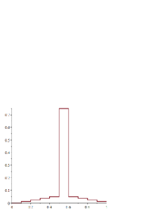
Figure 3. Density $f_{B}=f_{0a}$ invariant for map $g$

Example 2.

For a specific example we fix $N=10$. We consider density $f_{B}=f_{0,a}$ corresponding to the vector $v=\frac{1}{80}[0,1,2,3,4,60,4,3,2,1]$ (Figure 3). The semi-Markov map $g$ constructed as above is shown in Figure 4.

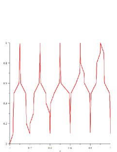
Figure 4. Semi-Markov map $g$ preserves density $f_{B}$

The maps $T$ and $T\varepsilon$ are shown in Figures 5 and 6.

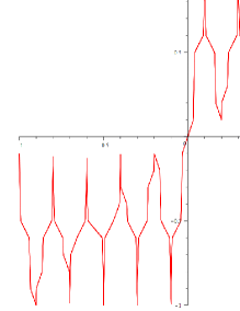
Figure 5. Map $T$ preserves two densities: $f_{B}$ and symmetric $f_{A}$

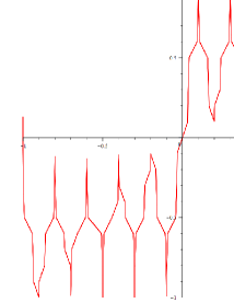
Figure 6. Metastable map $T_{\varepsilon}$ preserves unique density                          $f_{\varepsilon}\sim\frac{1}{2}f_{A}+\frac{1}{2}f_{B}$

The computer simulation of the density $f_{\varepsilon}\sim\frac{1}{2}f_{A}+\frac{1}{2}f_{B}$ is shown in Figure 7.

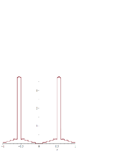
Figure 7. Metastable map $T_{\varepsilon}$ preserves unique density                          $f_{\varepsilon}\sim\frac{1}{2}f_{A}+\frac{1}{2}f_{B}$

5. Conflict of Interest

On behalf of all authors, the corresponding author states that there is no conflict of interest.

References

- [1] A. Boyarsky and P. Góra, A dynamical systems model for interference effects and the two-slit experiment of quantum physics, Phys. Lett. A, 168, 103–112, 1992.
- [2] MR1461536 Boyarsky, Abraham, Góra, Pawel, Laws of chaos. Invariant measures and dynamical systems in one dimension, Probability and its Applications. Birkhäuser Boston, Inc., Boston, MA, 1997.
- [3] Tim Folger, Crossing the quantum divide, Scientific American, July 2018, 29–35.
- [4] Cecilia Gonzáles-Tokman, Brian R. Hunt and Paul Wright, Approximating invariant densities of metastable systems, Ergod. Th. & Dynamic Sys., 31, 1345–1361, 2011.
- [5] MR1129877 Góra, P., Boyarsky, A., A matrix solution to the inverse Perron-Frobenius problem, Proc. Amer. Math. Soc. 118 (1993), no. 2, 409–414.
- [6] MR1244104 Lasota, Andrzej, Mackey, Michael C., Chaos, fractals, and noise. Stochastic aspects of dynamics, Second edition. Applied Mathematical Sciences, 97. Springer-Verlag, New York, 1994.
- [7] MR2355244 Rogers, Alan, Shorten, Robert, Heffernan, Daniel M., A novel matrix approach for controlling the invariant densities of chaotic maps, Chaos Solitons Fractals 35 (2008), no. 1, 161–175.