On-the-fly Global Embeddings Using
Random Projections for Extreme Multi-label Classification

Abstract

The goal of eXtreme Multi-label Learning (XML) is to automatically annotate a given data point with the most relevant subset of labels from an extremely large vocabulary of labels (e.g., a million labels). Lately, many attempts have been made to address this problem that achieve reasonable performance on benchmark datasets. In this paper, rather than coming-up with an altogether new method, our objective is to present and validate a simple baseline for this task. Precisely, we investigate an on-the-fly global and structure preserving feature embedding technique using random projections whose learning phase is independent of training samples and label vocabulary. Further, we show how an ensemble of multiple such learners can be used to achieve further boost in prediction accuracy with only linear increase in training and prediction time. Experiments on three public XML benchmarks show that the proposed approach obtains competitive accuracy compared with many existing methods. Additionally, it also provides around 6572$\times$ speed-up ratio in terms of training time and around 14.7$\times$ reduction in model-size compared to the closest competitors on the largest publicly available dataset.

I Introduction

eXtreme Multi-label Learning (or XML) is the problem of learning a classification model that can automatically assign a subset of the most relevant labels to a data point from an extremely large vocabulary of labels. With a rapid increase in the digital content on the Web, such techniques can be useful in several applications such as indexing, tagging, ranking and recommendation, and thus their requirement is becoming more and more critical. E.g., Wikipedia contains more than a million labels and one might be interested in learning a model using the Wikipedia articles and corresponding labels, so that it can be used to automatically annotate a new article with a subset of the most relevant labels. Another example can be to display a subset of advertisements to online users based on their browsing history. It is important to note that multi-label classification is different from multi-class classification that aims at assigning a single label/class to a data point.

While XML has several applications, it is a challenging problem as it deals with a very large number (hundreds of thousands, or even millions) of data points and features, and a practically unimaginable size of the output space (exponential in terms of vocabulary size). As a result, recently this has been approached using several interesting techniques such as [1, 2, 3, 4, 5, 6, 7, 8, 9, 10, 11, 12, 13, 14, 15, 16], most of which try to capture the relationships between features and labels. Moreover, these also attempt to address the scalability aspect that is particularly critical in the XML task, and is usually achieved by making an extensive use of computational resources. While many of these techniques have shown good performance, one thing that is missing in the XML literature is comparison with a conceptually simple and computationally light technique that can justify the need for complex models and resource-intensive training. In this paper, we are interested in investigating a simple approach for XML that can fill this gap and thus serve as a baseline for this task.

With this objective, we present On-the-fly Global Embeddings for Extreme Classification (OGEEC, pronounced as “o-geek”), an XML classifier than can quickly generate a global and structure preserving feature embedding, and easily scale to very large datasets using limited computational resources. We start by posing XML as a retrieval task where given a new data point, we retrieve its k-nearest neighbours from the training set, and then perform a weighted propagation of the labels from the nearest points to the input point based on their degree of similarity. While this idea sounds simple and straightforward, applying this directly in XML is practically difficult, because computing the nearest neighbours from a large training set in a very high-dimensional feature space (both are of the order $10^{5}-10^{6}$) is computationally prohibitive [2, 1, 8]. To address this, we adopt a global and linear feature embedding technique that performs an inherently non-linear projection of a high-dimensional data into a lower dimensional space. This computationally linear yet inherently non-linear projection can be computed in a couple of seconds (hence we call it on-the-fly), and also preserves pairwise distances among data points within a certain error bound, thus allowing efficient computation of the nearest neighbours in a low-dimensional (of the order $10^{2}$) latent embedding space. Precisely, this embedding is inspired from the strong theoretical properties of the JL-Lemma [17], and is quite simple: compute a matrix whose entries are independently sampled from the Normal distribution, and use it for feature projection/embedding into a lower dimensional space. It is interesting to note here that while this embedding is obtained without using the training data, it is still capable of preserving the structure of the data, thanks to the large sample-size in XML. In other words, while an extremely large amount of data in XML becomes a challenge for other learning techniques, it is conducive for applying the JL-Lemma. Further, to safeguard against the randomness that is implicit in the process of generating an embedding, we generate an ensemble of embeddings (or learners) by doing multiple samplings from the Normal distribution. Our empirical analyses demonstrate that using such ensembles leads to not only stable solutions with only linear increase in training and prediction time but also significant increase in prediction accuracies which are quite competitive (and many a times even better) compared to the state-of-the-art XML methods.

To summarize, the contributions of this paper are: (1) We present OGEEC classifier for XML which is simple, accurate, and thus can be used as a baseline for comparing other XML algorithms. To demonstrate the little resource requirements of OGEEC, we conduct all the experiments (both training as well as testing) on a single CPU core of an eight-core desktop (Intel i$7$-$7700$ $3.60$GHz $\times$ $8$ processor and $15.6$ GB RAM). (2) We supplement the study with extensive experimental analyses and comparisons with several state-of-the-art XML methods on three large-scale and benchmark XML datasets (Delicious-200K, Amazon-670K and Amazon-3M).

II Related Work

The XML problem has been approached by both non-deep learning based as well as deep learning based approaches. Among the non-deep learning based approaches, the three broad sub-categories include feature embedding-based approaches [1, 2, 18, 8], linear (one-vs-all) classification-based approaches [5, 6, 7, 19], and tree-based approaches [20, 4, 3, 21, 12, 22, 11]. Among the deep learning based approaches, the existing approaches can be categorized on the basis of whether they learn global features [9, 10, 15, 16] or local/attention-based features [14, 13].

The embedding based approaches focus on reducing the effective number of features, labels or both by projecting them into a lower dimensional space. Among the initial approaches such as LPSR-NB [20], LEML [2] and REML [18], while LPSR-NB uses label hierarchies to iterative partition the label space, LEML and REML learn to project label-matrix into a low-rank structure and perform a projection back into the original label space during prediction. Recently, SLEEC [1] and AnnexML [8] have been considered as the representative methods in this category. These consist of three steps: clustering the samples, learning a non-linear low-dimensional feature embedding for each cluster, and kNN-based classification. During training, the low-dimensional embedding is learned such that it preserves pairwise distances between closest label vectors, thus capturing label correlations. The clustering of training samples helps in speeding-up the testing process, as the neighbours of a test sample are computed only from the group to which it belongs. The difference between them is that SLEEC aims at preserving pairwise distances wheres AnnexML uses a graph embedding method such that the k-nearest neighbour graph of the samples is preserved. Since clustering high-dimensional features is usually unstable, both SLEEC as well as AnnexML further use an ensemble of such learners by using different clusterings, and the predictions from all the learners in an ensemble are averaged to get the final prediction.

The linear classification-based approaches such as [5, 19, 6, 7] learn a linear classifier per label, with the difference being in the form of loss function and constraints imposed on the classifier. DiSMEC [5] learns max-margin classifiers using the conventional hinge-loss and L2-norm regularization. To scale this to large vocabularies, it uses few hundreds of CPU cores in parallel. Before testing, the dimensions in each classifier which have negligible magnitude are explicitly omitted for speed-up. To address this, L1-norm regularization is adopted in ProXML [19] that helps in learning sparse classifiers, which is also shown to be helpful in boosting the prediction accuracy of rare labels. In PD-Sparse [6] and PPD-Sparse [7], negative-sampling through a sparsity preserving optimization is used to reduce the training-time, and heuristic-based feature sampling is performed to reduce the prediction time. In general, while these approaches achieve high prediction accuracies, their training and prediction times increase significantly and it may take several weeks to train these models on large vocabulary datasets.

The third direction is based on tree based approaches such as [23, 24, 20, 4, 3, 21, 11, 12, 22] that perform hierarchical feature/label-based partitioning for fast training and prediction. However, due to the cascading effect, an error made at a top level propagates to lower levels. Among these, FastXML [4], PfastreXML [3] aim at optimizing label ranking by recursively partitioning the feature space. However, since these learn a weak classifier at each node in a tree for fast traversal, this affects their prediction accuracy. This is overcome in a recent hybrid approach method Parabel [11] that learns high-dimensional binary classifiers similar to [5] for label partitioning at each node and achieves promising results, though with increased complexity and memory requirements. Taking motivation from these methods, other methods such Slice [22] and Bonsai [12] try to address some of their limitations. E.g., in Slice [22], rather than learning a classfier for label partitioning using all the labels, only the most confusing labels are used that are identified using an efficient negative sampling technique. Similarly, in Bonsai [12], rather than learning a deep but narrow tree, a shallow but relatively wider tree is learned by clustering the label representations using the k-means algorithm.

While non-deep learning based methods discussed above have rely on bag-of-words features, deep learning based methods use raw input to learn dense representations using multiple non-linear transformations that can effectively capture semantic as well as contextual information. One of the first such methods for XML was XML-CNN [9] which uses 1-D CNN along both word embedding dimension and sequence length. The dense embedding learned by XML-CNN is also used in SLICE as discussed above that learns a tree-based model. Another approach DeepXML [10] was the first to learn deep feature embedding in XML by using a label graph structure. A recent approach APLC-XLNet [16] fine-tunes a generalized autoregressive pre-trained model XLNet [25] and forms clusters of labels based on label distribution to approximate the cross-entropy loss. Among the attention-based methods that learn local features, AttentionXML [14] uses BiLSTMs and label-aware attention, while X-Transformer [13] pre-trained using the BERT transformer model [26]. In general, while these methods achieve good empirical results, their models are quite heavy with few hundreds/thousands of millions of learned parameters and are thus computationally demanding (with some of them requiring a cluster of GPUs for execution). In later parts of the paper, we will contrast our approach with these methods as well as analyze the pros and cons of each.

III The OGEEC Approach

In this section, we describe the proposed OGEEC approach. Let $\mathcal{D}=\{(\mathbf{x}_{1},\mathbf{y}_{1}),\ldots,(\mathbf{x}_{n},\mathbf{y}_{n})\}$ denote the training set, where $\mathbf{x}_{i}\in\mathcal{X}\subseteq\mathbb{R}^{d}$ is a $d$-dimensional feature vector and $\mathbf{y}_{i}\in\mathcal{Y}\subseteq\{0,1\}^{L}$ is the corresponding binary label vector that denotes the labels assigned to $\mathbf{x}_{i}$, with $1$ denoting the presence and $0$ denoting the absence of the corresponding label. Let $\mathbf{X}=[\mathbf{x}_{1};\ldots;\mathbf{x}_{n}]\in\mathbb{R}^{d\times n}$ be the data matrix whose each column is a feature vector.

One of the simplest learning based technique that can be employed to project high-dimensional features into a lower dimensional space is Principal Component Analysis (PCA) [27]. Though simple, the operations involved in PCA (such as eigenvalue decomposition) are quite expensive (in terms of both computation and memory), and can scale to only a few tens of thousands of feature dimensions [28, 29] with heavy computation and memory requirements. Due to this, it is not feasible to use PCA for dimensionality reduction when the dimensionality of input features is in several hundreds of thousands or even millions as in XML. . On the other hand, Johnson and Lindenstrauss [17] showed that the structure of high-dimensional data is well preserved in a lower dimensional space projected using random linear projections. As a result, random projections have been proven to be useful in a variety of applications such as dimensionality reduction, clustering [30], denstiy estimation [31], etc. Below, we first give an overview of the JL-Lemma, and then present the proposed approach.

III-A Background: Johnson-Lindenstrauss Lemma (or JL-Lemma)

When we seek a dimensionality reduction where the goal is to preserve the structure of the data by preserving pairwise distances between the data points, we can make use of a projection matrix that is randomly initialized in a particular way. This is also known as the random projection method, and is studied under the JL-Lemma [17]. Suppose we are initially given $n$ data points $\mathbf{x}_{1},\ldots,\mathbf{x}_{n}\in\mathbb{R}^{d}$ in a $d$-dimensional space, and we are interested in projecting these points into a lower dimensional space and find $n$ points $\mathbf{a}_{1},\ldots,\mathbf{a}_{n}\in\mathbb{R}^{r}$, where $r<<d$, such that

$$||\mathbf{a}_{j}||\;\;\approx\;\;||\mathbf{x}_{j}||\;\;\;\forall j,$$

$$||\mathbf{a}_{i}-\mathbf{a}_{j}||\;\;\approx\;\;||\mathbf{x}_{i}-\mathbf{x}_{j}||\;\;\;\forall i,j.$$

where $||\mathbf{x}||$ denotes the Euclidean norm of the vector $\mathbf{x}$. Then, the JL-Lemma is given as follows:

Theorem 1

Let $\mathbf{x}_{1},\ldots,\mathbf{x}_{n}\in\mathbb{R}^{d}$ be arbitrary. Pick any $\epsilon=(0,1)$. Then for some $r=O(log(n)/\epsilon^{2}$) there exist points $\mathbf{a}_{1},\ldots,\mathbf{a}_{n}\in\mathbf{R}^{r}$ such that

$$(1-\epsilon)||\mathbf{x}_{j}||\leq||\mathbf{a}_{j}||\leq(1+\epsilon)||\mathbf{x}_{j}||,\forall j$$

$$(1-\epsilon)||\mathbf{x}_{i}-\mathbf{x}_{j}||\leq||\mathbf{a}_{i}-\mathbf{a}_{j}||\leq(1+\epsilon)||\mathbf{x}_{i}-\mathbf{x}_{j}||,\forall i,j.$$ (1)

Moreover, in polynomial time we can compute a linear transformation $\mathbf{F}:\mathbb{R}^{d}\rightarrow\mathbb{R}^{r}$ such that, defining $\mathbf{a}_{j}=\mathbf{F}(\mathbf{x}_{j})$, the inequalities in the above equation are satisfied with probability at least $1-2/n$.

This implies that the linear transformation $\mathbf{F}$ can be used for projecting the initial data points into a lower dimensional space such that their pairwise distances are preserved within an error bound. In practice, the linear transformation $\mathbf{F}$ is a matrix whose entries are independent random variables sampled from a Normal distribution [32]. It is also important to note that the projected points $\{\mathbf{a}_{1},\ldots,\mathbf{a}_{n}\}$ have no dependence on the dimensionality of the input samples (i.e., $d$), which implies that the original data could be in an arbitrarily high dimensional space, thus making it suitable for XML. Another important thing is that while PCA is useful only when the original data points inherently lie on a low dimensional manifold, this condition is not required by the JL-Lemma.

Algorithm 1: Obtaining a single feature embedding matrix
Require:
(1) Training feature matrix: $\mathbf{X}=[\mathbf{x}_{1};\ldots;\mathbf{x}_{n}]\in\mathbb{R}^{d\times n}$
(2) Embedding dimension: $r$ ($r\leq d$)
Method:
Step-1: Compute matrix: $\mathbf{F}=normrnd(0,1,r,d)$
// in MATLAB
Post-processing:
Step-1: Normalize training features $\mathbf{X}$ using $\text{L}_{\text{2}}$-normalization
Step-2: $\mathbf{X}\leftarrow(\mathbf{X}^{T}\times\mathbf{F})^{T}$
Step-3: Re-normalize training features $\mathbf{X}$ using $\text{L}_{\text{2}}$-normalization

III-B Feature Embedding

Taking motivation from the JL-Lemma, we adopt a simple and easy to implement approach for generating a linear yet inherently non-linear and structure preserving projection matrix: we compute a matrix of random numbers generated from the Normal distribution (i.e., a Gaussian distribution with zero mean and unit variance, and use this to perform a linear projection of high ($d$-) dimensional input features into a lower ($r$-) dimensional latent embedding space, keeping $r<<d$. It is easy to note that obtaining this projection matrix does not involve any learning based on the given training data points. For completion, Algorithm 1 summarizes the steps of obtaining a single such global embedding. Later, in Section IV-A1, we will discuss the error bounds of the pairwise distances for different datasets and using different projection matrices.

TABLE I: Multi-label datasets used for empirical analysis in this paper (available at the Extreme Classification Repository [33]). ASpL and ALpS denote the average number of samples per label and average number of labels per sample respectively

Dataset	# Training Samples	# Test Samples	# Features	# Labels	ASpL	ALpS
Delicious-200K	196,606	100,095	782,585	205,443	72.29	75.54
Amazon-670K	490,449	153,025	135,909	670,091	3.99	5.45
Amazon-3M	1,717,899	742,507	337,067	2,812,281	31.64	36.17

Next, in order to control the randomness involved in this process and achieve stable predictions, we obtain a set of multiple such global feature embeddings (learners) by using different random samplings from the Normal distribution. In particular, we do this by using different “seed” values for initializing random matrices.

Algorithm 2: Label prediction using a single embedding
Require:
(1) Test point $\mathbf{x}_{t}\in\mathbb{R}^{d}$
(2) Number of nearest neighbours: $k$
(3) Projected and normalized training features $\mathbf{X}$
(4) Feature embedding matrix: $\mathbf{F}$
Pre-processing:
Step-1: Normalize $\mathbf{x}_{t}$ using $\text{L}_{\text{2}}$-normalization
Method:
Step-1: $\mathbf{x}_{t}\leftarrow(\mathbf{x}_{t}^{T}\times\mathbf{F})^{T}$
Step-2: Normalize $\mathbf{x}_{t}$ using $\text{L}_{\text{2}}$-normalization
Step-3: Compute the $k$-nearest neighbours of $\mathbf{x}_{t}$ from $\mathbf{X}$ using dot-product
Step-4: Propagate the labels from the neighbours by weighting them with the corresponding similarity scores

III-C Label Prediction

III-C1 Using a single embedding

For label prediction, we use a weighted k-nearest neighbour based classifier to propagate labels to a new sample from its few nearest neighbours in the training set. For each label, we use Bernoulli models, considering either presence or absence of labels in the neighbourhood [34].

Let $\mathbf{x}_{t}$ denote a test sample, $\mathcal{N}^{k}_{t}$ denote the set of its $k$ nearest neighbours from the training set (with similarity being computed using dot-product), and $y^{w}\in\{0,1\}$ denote the presence/absence of the label corresponding to index $w$ for a sample $\mathbf{x}$. Then, the label presence prediction for $\mathbf{x}_{t}$ is defined as a weighted sum over the training samples in $\mathcal{N}^{k}_{t}$:

$$p(y^{w}_{t}=1|\mathbf{x_{t}}) \propto \sum_{\mathbf{x}_{i}\in\mathcal{N}^{k}_{t}}\pi_{it}\;p(y^{w}_{i}=1|\mathbf{x}_{i}),$$ (2)

$$p(y^{w}_{i}=1|\mathbf{x}_{i}) = \left\{\begin{array}[]{rl}1&\text{for}\;y^{w}_{i}=1,\\ 0&\text{otherwise,}\end{array}\right.$$ (5)

where $\pi_{it}$ denotes the importance of the training sample $\mathbf{x}_{i}$ in predicting the labels of the test sample $\mathbf{x}_{t}$, and is given by $\pi_{it}=max(\mathbf{x}_{i}^{T}\mathbf{x}_{t},0)$. Since we assume the samples to be $\text{L}_{\text{2}}$-normalized, this is equivalent to computing the cosine similarity score between them. Using Eq. 2, we get prediction scores for all the labels and pick the top-$K$ ($K\in\{1,3,5\}$) for assignment and performance evaluation. It is important to note that while we do not explicitly model the dependencies among labels in the training data, these are implicitly exploited in our model. This is because the labels that co-occur in a given training sample get the same weight depending on the degree of similarity of that training sample with the test sample, thus implicitly capturing sample-to-sample, sample-to-label as well as label-to-label similarities. Algorithm 2 summarizes the steps of label prediction using a single learner. In case of multiple learners, we use Eq. 2 to get the prediction scores for all the labels using each learner individually. Then we average these prediction scores over all the learners in an ensemble, and pick the top few labels for assignment and performance evaluation.

III-D Relation with deep learning based methods

In the last few years, deep learning based methods have become popular for several tasks, particularly those that involve classification. These methods aim at learning characteristics/features that are distinctive across categories. To do so, they learn a highly non-linear transformation function of the input data. The global embedding technique used in OGEEC shares a similar objective (specifically, with deep metric learning based methods) in the sense that it also involves an inherently non-linear and structure-preserving mapping of features. However, in contrast to deep learning based methods that rely on an extensive use of training data and compute resources, the global embedding used in OGEEC relies on the distributional properties of an extremely large data set in a high-dimensional space which are guaranteed by the JL-Lemma. This enables OGEEC to obtain a data-independent linear transformation that is inherently non-linear and structure-preserving. As we will discuss in Section IV-C, despite learning the transformation function without making use of training data, OGEEC still performs fairly well in comparison to deep learning based XML methods.

IV Experiments

IV-A Experimental Set-up

IV-A1 Datasets and Analysis

We use three large-scale XML datasets in our experiments: Delicious-200K, Amazon-670K and Amazon-3M, available at the Extreme Classification Repository [33]. Among these, Amazon-670K and Amazon-3M are the top-two largest public XML datasets. We use the same training and test partitions as given in the repository, and do not use any additional meta-data. The statistics of these datasets are summarized in Table I. For all the datasets, we use the pre-computed bag-of-words features available at the above repository.

TABLE II: Error bounds of the pairwise distances (Eq. 1) for different datasets by considering $r=200$

Dataset	${\epsilon}$	${1-\epsilon}$	${1+\epsilon}$
Delicious-200K	0.1627	0.8373	1.1627
Amazon-670K	0.1687	0.8313	1.1687
Amazon-3M	0.1766	0.8234	1.1766

TABLE III: Error bounds of the pairwise distances for the Delicious-200K dataset by varying the dimensionality of the projection space in $\{50,100,\ldots,400\}$

Output Ftr. Dimension ($r$)	${\epsilon}$	${1-\epsilon}$	${1+\epsilon}$
50	0.3254	0.6746	1.3254
100	0.2301	0.7699	1.2301
150	0.1879	0.8121	1.1879
200	0.1627	0.8373	1.1627
250	0.1455	0.8545	1.1455
300	0.1328	0.8672	1.1328
350	0.1230	0.8770	1.1230
400	0.1150	0.8850	1.1150

TABLE IV: Performance of OGEEC in terms of Precision@$K$, nDCG@$K$, propensity-scored Precision@$K$, and propensity-scored nDCG@$K$ ($K$=1,3,5). In case of “One learner”, the accuracies are averaged over five individual learners. In case of “Five learners”, the accuracies are calculated after fusing the predictions obtained using five individual learners as described in Section III-B

		One learner				Five learners
Dataset	Metric$@K$	Prec.	nDCG	PS-Prec.	PS-nDCG	Prec.	nDCG	PS-Prec.	PS-nDCG
Delicious-200K	@1	36.89$\pm$0.11	36.89$\pm$0.11	5.83$\pm$0.02	5.83$\pm$0.02	40.54	40.54	6.37	6.37
	@3	30.86$\pm$0.04	32.28$\pm$0.05	6.26$\pm$0.01	6.14$\pm$0.01	34.25	35.74	6.91	6.76
	@5	27.79$\pm$0.02	29.91$\pm$0.03	6.62$\pm$0.01	6.39$\pm$0.01	30.97	33.22	7.33	7.05
Amazon-670K	@1	35.21$\pm$0.06	35.21$\pm$0.06	21.84$\pm$0.06	21.84$\pm$0.06	37.45	37.45	23.05	23.05
	@3	31.98$\pm$0.02	33.77$\pm$0.02	24.89$\pm$0.04	24.09$\pm$0.03	33.67	35.64	26.19	25.37
	@5	29.73$\pm$0.03	33.00$\pm$0.03	28.05$\pm$0.03	26.21$\pm$0.03	31.12	34.68	29.42	27.54
Amazon-3M	@1	36.31$\pm$0.04	36.31$\pm$0.04	12.06$\pm$0.02	12.06$\pm$0.02	40.57	40.57	12.87	12.87
	@3	34.15$\pm$0.01	34.99$\pm$0.01	14.22$\pm$0.01	13.67$\pm$0.01	37.95	38.96	15.24	14.63
	@5	32.58$\pm$0.01	34.12$\pm$0.01	15.87$\pm$0.00	14.83$\pm$0.01	36.10	37.91	17.04	15.90

In Table II, we present the error bounds of the pairwise distances for different datasets by using $\epsilon=\sqrt{log(n)/d}$ (for simplicity, we omit the $O(\cdot)$ notation), where $n$ is the number of data points (training samples) and $d$ is the dimensionality of the input feature space. We consider the dimensionality of the (output) projection space as $r=200$, which is what we use to evaluate and compare the performance of OGEEC. Here, we observe that the error bounds ($1-\epsilon$ and $1+\epsilon$) are comparable for all the datasets, and quite reasonable even when the dimensionality of the projection space is just $200$. To further investigate this, we vary the dimensionality of the projection space in $r=\{50,100,\ldots,400\}$ for the Delicious-200K dataset in Table III. We observe that as we increase $r$, the value of $\epsilon$ reduces and becomes half as we move from $r=50$ to $r=200$ (from $0.3254$ to $0.1627$), however the rate of reduction slows down after that. As we will see later in our experiments, we observe similar trends in accuracies (Figure 1) where they increase steeply in the beginning on increasing $r$ and then start levelling-out. Because of this, we fix the dimensionality of the output/projection space as $r=200$ in all the reported results, which also provides a reasonable prediction time for all the datasets.

IV-A2 Evaluation Metrics

Following existing methods methods [1, 4, 3, 5, 6, 2, 11, 19] and the evaluation metrics published on the XML repository [33], we use four metrics in our evaluations: Precision at $K$ (P@$K$), nDCG at $K$ (N@$K$), propensity-scored Precision at $K$ (PSP@$K$) and propensity-scored nDCG at $K$ (PSN@$K$), for $K\in\{1,3,5\}$. P@$K$ and PSP@$K$ metrics count the percentage of correctly predicted labels among the top $K$ labels, without considering the rank of correct labels among the predictions. N@$K$ and PSN@$K$ are ranking based measures and also take into account the position of correct labels among the top $K$ labels, with correct labels towards the top being considered better than those predicted towards the bottom of the top $K$ predictions. PSP@$K$ and PSN@$K$ were proposed in [3], which balance the correct prediction of rare and frequent labels by fitting a sigmoid function on the frequency distribution of the labels in the training set, and then use it to scale the prediction scores of labels.

IV-A3 Hyperparameters

In all the main results and comparisons of OGEEC, we keep the dimensionality of the latent feature embedding space as $r=200$, the number of nearest neighbours in kNN as $k=5$, and an ensemble of five learners. These are chosen from a held-out validation set of the Delicious-200K dataset, and the same values are used for the other two data sets.

IV-B Performance of OGEEC

IV-B1 Results

Table IV shows the performance of OGEEC in terms of all the four evaluation metrics using one learner and an ensemble of five learners. From these results, we can make the following observations: (1) As discussed earlier in Section I, even though the global feature embedding used in OGEEC is computed without using the training data, it achieves reasonable results on all the datasets, thus validating the promise of the JL-Lemma on the challenging XML task, and large-scale learning problems in general. (2) The variation in the performance of individual learners is statistically significant ($p$-value $<0.001$), with very small standard deviation. On using an ensemble of multiple learners, there is always a boost in the accuracy (by up to $\sim 4\%$ absolute in some cases). (3) The accuracy trends are similar across all the metrics and datasets, which demonstrate a consistent behaviour by OGEEC.

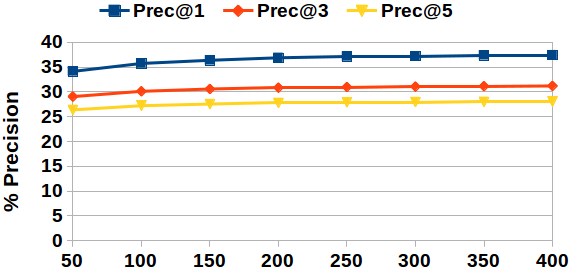
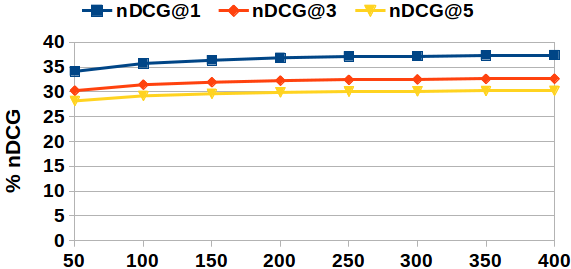
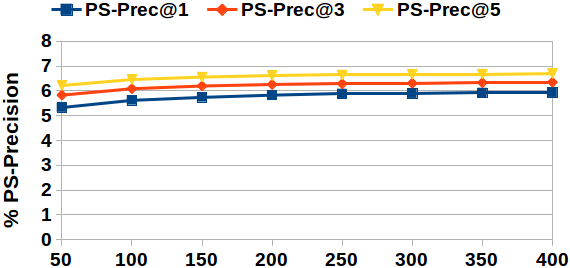
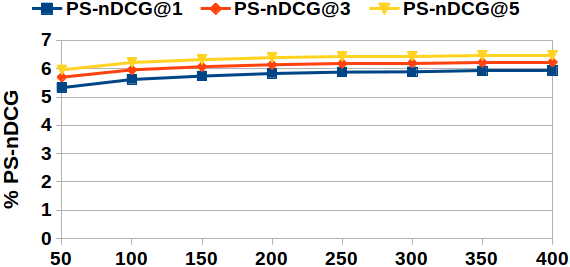
Figure 1: Performance of OGEEC on the Delicious-200K dataset by varying the dimensionality of the embedding space in $\{50,100,150,200,250,300,350,400\}$ using one learner.

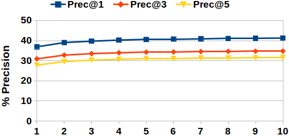
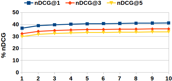
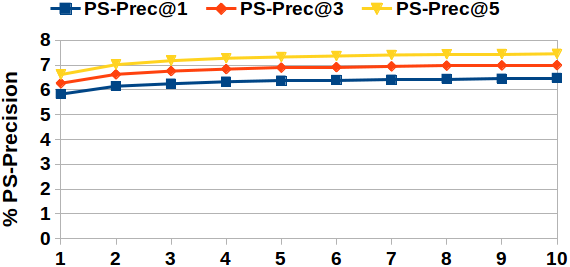
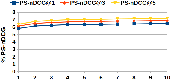
Figure 2: Performance of OGEEC on the Delicious-200K dataset by varying the number of learners in {1, 2,…,10} with $r=200$.

IV-B2 Ablation Studies

In Figure 1, we study the influence of the dimensionality of the latent embedding space on the Delicious-200K dataset. To do so, we vary the embedding dimension in $\{50,100,\ldots,400\}$ and evaluate the performance of OGEEC using one learner. Here, we observe that the results using all the metrics consistently increase as we increase the embedding dimension, which is expected since the loss in information reduces with an increase in the number of dimensions. We also see that the improvements are steeper in the beginning and then gradually saturate. In Figure 2, we study the influence of the number of learners in an ensemble by varying them in $\{1,2,\ldots,10\}$ on the Delicious-200K dataset. Here also, we observe that the accuracy increases sharply in the beginning and then starts saturating after training very few learners. In both these experiments, it is important to note that the computation cost increases with an increase in the dimensionality of the latent embedding space as well number of learners in an ensemble. Hence, based on the results in these experiments, we set the embedding dimension as $200$ and number of ensemble as $5$ in all our experiments to manage the trade-off between accuracies and computation cost.

TABLE V: Computation time of OGEEC using one learner. Both training and prediction times are using a single CPU core with $15.6$ GB RAM.

Dataset	Training time (sec.)	Prediction time
		per sample (sec.)
Delicious-200K	2.46	0.48
Amazon-670K	0.54	0.48
Amazon-3M	1.14	2.63

TABLE VI: Model details of OGEEC using one learner. # P: No. of parameters (= Feature embedding matrix size); # LP: No. of learned parameters; # HP: No. of hyper-parameters

Dataset	# P	# LP	# HP
Delicious-200K	782585 $\times$ 200	0	2
Amazon-670K	135909 $\times$ 200	0	2
Amazon-3M	337067 $\times$ 200	0	2

TABLE VII: Comparison between LSH and OGEEC in terms of prediction accuracies and experimental requirements on the Delicious-200K dataset

Metric	LSH	OGEEC (Ours)
P@1	38.90	40.54
P@3	33.02	34.25
P@5	30.07	30.97
N@1	38.90	40.54
N@3	34.40	35.74
N@5	32.12	33.22
PSP@1	6.04	6.37
PSP@3	6.60	6.91
PSP@5	7.07	7.33
PSN@1	6.04	6.37
PSN@3	6.45	6.76
PSN@5	6.77	7.05
Model Size (GB)	1.50	2.64
Training Time (sec)	2.46	37.49
Prediction Time (sec)	0.48	0.13

IV-B3 Computation time and Model details

We show the training and prediction time of OGEEC in Table V, and the model details in terms of the number of parameters (which is also the size of the feature embedding matrix $\mathbf{F}$), the number of learned parameters, and the number of hyper-parameters in Table VI. Here, the training and prediction time denote the time taken for processing the step(s) under “Method” in the corresponding algorithm (c.f. Algorithm-1 and Algorithm-2). The column “# Learned Parameters” denotes the number of parameters in the embedding matrix that are learned using the training data, which is essentially zero in OGEEC. The significance of this is to specifically highlight that OGEEC requires only the dimensionality of the input feature space and the latent embedding space to obtain the projection matrix, without the need of training data. This is a unique property of OGEEC that makes it the first such technique in the XML literature as per our knowledge. From Table V, we can notice that the prediction in OGEEC is also reasonably fast given the fact that we propagate labels after doing an exhaustive matching with all the training samples on just one CPU core (e.g., with $\sim 1.7$ million samples in the Amazon-3M dataset). In practice, the prediction time depends primarily on two factors: exact search of the nearest neighbours from the entire training set (which increases as the number of training samples increases), and propagation of labels from the identified nearest neighbours (which increases as the vocabulary size increases). At the time of deployment, we can reduce the prediction time significantly by first retrieving the nearest neighbours on subsets of training data in parallel, and then doing a second filtering in one pass after merging those small subsets. In a preliminary experiment, we observed that the prediction time of OGEEC on the Amazon-3M dataset can be brought down from $\sim 2.6$ seconds per sample to an order of a few milliseconds without any compromise on accuracy by using a parallel version of the kNN algorithm on 24 CPU cores.

IV-B4 Comparison with Locality Sensitive Hashing

Locality Sensitive Hashing (LSH) is a popular algorithm for fast and approximate search of nearest neighbours, and has been used in a variety of applications. As we perform an exhaustive kNN search in the proposed OGEEC approach, we compare it with LSH to analyze the advantages as well as limitations of adopting a simple technique. For fair comparisons, we learn the hash tables in LSH using the features in the latent embedding space of OGEEC. In Table-VII, first we compare the accuracies of OGEEC and LSH. Here, we observe that OGEEC usually achieves provide $\sim 3-15\%$ of relative improvements compared to LSH. Next, we can observe that while the model-size of both OGEEC and LSH are comparable, the training time of OGEEC is much less than that of LSH. Finally, we found that the prediction time of OGEEC and LSH were of the same order. From these comparisons, we can conclude that while the time requirements of both OGEEC and LSH are comparable for practical applications, OGEEC provides a clear empirical advantage over LSH.

TABLE VIII: Comparison with non-deep learning based methods

Ours

Less than ours

Better than ours by up to 3%

Better than ours by 3–6%

Better than ours by 6–9%

Better than ours by ¿9%

Delicious-200K
Method	P@1	P@3	P@5	N@1	N@3	N@5	PSP@1	PSP@3	PSP@5	PSN@1	PSN@3	PSN@5
OGEEC (ours)	40.54	34.25	30.97	40.54	35.74	33.22	6.37	6.91	7.33	6.37	6.76	7.05
LPSR-NB	18.59	15.43	14.07	18.59	16.17	15.13	3.24	3.42	3.64	3.24	3.37	3.52
PD-Sparse*	34.37	29.48	27.04	34.37	30.60	28.65	5.29	5.80	6.24	5.29	5.66	5.96
LEML*	40.73	37.71	35.84	40.73	38.44	37.01	6.06	7.24	8.10	6.06	6.93	7.52
PfastreXML*	41.72	37.83	35.58	41.72	38.76	37.08	3.15	3.87	4.43	3.15	3.68	4.06
FastXML*	43.07	38.66	36.19	43.07	39.70	37.83	6.48	7.52	8.31	6.51	7.26	7.79
DiSMEC*	45.50	38.70	35.50	45.50	40.90	37.80	6.50	7.60	8.40	6.50	7.50	7.90
Bonsai*	46.69	39.88	36.38	46.69	41.51	38.84	7.26	7.97	8.53	7.26	7.75	8.10
AnnexML*	46.79	40.72	37.67	46.79	42.17	39.84	7.18	8.05	8.74	7.18	7.78	8.22
Parabel*	46.86	40.08	36.70	46.86	41.69	39.10	7.22	7.94	8.54	7.22	7.71	8.09
SLEEC*	47.85	42.21	39.43	47.85	43.52	41.37	7.17	8.16	8.96	7.17	7.89	8.44
Amazon-670K
Method	P@1	P@3	P@5	N@1	N@3	N@5	PSP@1	PSP@3	PSP@5	PSN@1	PSN@3	PSN@5
OGEEC (ours)	37.45	33.67	31.12	37.45	35.64	34.68	23.05	26.19	29.42	23.05	25.37	27.54
LEML*	8.13	6.83	6.03	8.13	7.30	6.85	2.07	2.26	2.47	2.07	2.21	2.35
LPSR-NB*	28.65	24.88	22.37	28.65	26.40	25.03	16.68	18.07	19.43	16.68	17.70	18.63
SLICE+FastText*	33.15	29.76	26.93	33.15	31.51	30.27	20.20	22.69	24.70	20.20	21.71	22.72
SLEEC*	35.05	31.25	28.56	34.77	32.74	31.53	20.62	23.32	25.98	20.62	22.63	24.43
FastXML*	36.99	33.28	30.53	36.99	35.11	33.86	19.37	23.26	26.85	19.37	22.25	24.69
PfastreXML*	39.46	35.81	33.05	39.46	37.78	36.69	29.30	30.80	32.43	29.30	30.40	31.49
AnnexML*	42.39	36.89	32.98	42.39	39.07	37.04	21.56	24.78	27.66	21.56	23.38	24.76
ProXML*	43.50	38.70	35.30	43.50	41.10	39.70	30.80	32.80	35.10	30.80	31.70	32.70
DiSMEC*	44.70	39.70	36.10	44.70	42.10	40.50	27.80	30.60	34.20	27.80	28.80	30.70
Parabel*	44.89	39.80	36.00	44.89	42.14	40.36	25.43	29.43	32.85	25.43	28.38	30.71
PPD-Sparse*	45.32	40.37	36.92	–	–	–	26.64	30.65	34.65	–	–	–
Bonsai*	45.58	40.39	36.60	45.58	42.79	41.05	27.08	30.79	34.11	–	–	–
Amazon-3M
Method	P@1	P@3	P@5	N@1	N@3	N@5	PSP@1	PSP@3	PSP@5	PSN@1	PSN@3	PSN@5
OGEEC (ours)	40.57	37.95	36.10	40.57	38.96	37.91	12.87	15.24	17.04	12.87	14.63	15.90
PfastreXML*	43.83	41.81	40.09	43.83	42.68	41.75	21.38	23.22	24.52	21.38	22.75	23.68
FastXML*	44.24	40.83	38.59	44.24	41.92	40.47	9.77	11.69	13.25	9.77	11.20	12.29
DiSMEC	47.34	44.96	42.80	47.36	–	–	–	–	–	–	–	–
Parabel*	47.48	44.65	42.53	47.48	45.73	44.53	12.82	15.61	17.73	12.82	14.89	16.38
Bonsai*	48.45	45.65	43.49	48.45	46.78	45.59	13.79	16.71	18.87	–	–	–
AnnexML*	49.30	45.55	43.11	49.30	46.79	45.27	11.69	14.07	15.98	–	–	–

IV-C Comparison with the state-of-the-art

Now we demonstrate the efficiency and effectiveness of the proposed OGEEC approach by comparing it with several non-deep learning based as well deep learning based state-of-the-art XML methods in terms of accuracies, model-size and training time. Among the non-deep learning based methods, we compare with LPSR-NB [20], LEML [2], SLEEC [1], AnnexML [8], PD-Sparse [6], PPD-Sparse [7], DiSMEC [5], ProXML [19], FastXML [4], PfastreXML [3], Parabel [11], Bonsai [12] and SLICE [22]. Among the deep learning based methods, we compare with XML-CNN [9], DeepXML [10], APLC-XLNet [16], Astec [15] X-Transformer [13], and AttentionXML [14]. For benchmarking, we adopt the results published on the XML repository [33].. For ease of comparisons, we highlight the results in different colors.

We first compare with non-deep learning based methods in Table VIII. In general, we notice that despite its simplicity, OGEEC achieves quite competitive results, which are many a times even better, compared to other methods all of which are algorithmically much more complex than it. We can also make several other observations from these results: (1) The accuracy of OGEEC in terms of propensity-scored metrics is particularly impressive, where it outperforms many of the existing methods. This indicates that our initial hypothesis of posing XML as a retrieval task and propagating labels from globally identified nearest neighbours in a low-dimensional structure-preserving space is in fact quite effective in boosting the accuracy of low-frequency labels. It should be noted that while the existing benchmark nearest-neighbour based approaches such as LEML [2], SLEEC [1] and AnnexML [8] have advocated the use of multiple local feature embeddings, ours is the first attempt that demonstrates the effectiveness of using a global structure-preserving feature embedding in the XML task as per our knowledge. (2) Similarly, using non-propensity scored measures, the accuracy of OGEEC is quite impressive. For most of the cases where OGEEC is outperformed by other methods, the difference in accuracy is below $6\%$ despite elaborate modelling and training efforts. We acknowledge that a performance gap by a few percentage might be critical in certain applications, however comparisons with a simple approach like OGEEC would help in better understanding and appreciating the benefits of the sophisticated modelling and training procedures used by the existing methods. (3) Among the existing embedding based methods, only AnnexML could scale to the largest Amazon-3M dataset Similarly, among the linear one-vs.-all classifier based approaches such as DiSMEC, ProXML, PD-Sparse and PPD-Sparse, only DiSMEC could be scaled on this dataset by using multiple CPU core (if we had used one CPU core, the training time of DiSMEC would have been $\approx 4995$ hours). Only the tree-based approaches such as FastXML, PfastreXML and Parabel that partition the label-space in a hierarchical manner could manage to scale to this dataset (e.g., the training time of PfastreXML is $\approx 15$ hours using $16$ CPU cores). On the other hand, OGEEC, being an embedding-based approach, easily scales to this dataset and is able to generate an ensemble of five learners in just few seconds (c.f. Table V) using just one CPU core and $15.6$ GB RAM. (4) On the Amazon-3M dataset, the performance of OGEEC is quite reasonable. In terms of P@K and N@K, it is quite close to FastXML and PfastreXML, and competitive to other methods. In terms of PSP@K and PSN@K, the accuracy of OGEEC is better than FastXML and AnnexML, comparable to Parabel and Bonsai, and competitive to PfastreXML. Here, it is worth noting that AnnexML is the current state-of-the-art non-deep learning based embedding approach for XML, and is the closest competitor to OGEEC.

TABLE IX: Comparison with deep learning based methods

Ours

Less than ours

Better than ours by up to 3%

Better than ours by 3–6%

Better than ours by 6–9%

Better than ours by ¿9%

Delicious-200K
Method	P@1	P@3	P@5	N@1	N@3	N@5	PSP@1	PSP@3	PSP@5	PSN@1	PSN@3	PSN@5
OGEEC (ours)	40.54	34.25	30.97	40.54	35.74	33.22	6.37	6.91	7.33	6.37	6.76	7.05
X-Transformer*	45.59	39.10	35.92	45.59	40.62	38.17	6.96	7.71	8.33	6.96	7.47	7.86
Amazon-670K
Method	P@1	P@3	P@5	N@1	N@3	N@5	PSP@1	PSP@3	PSP@5	PSN@1	PSN@3	PSN@5
OGEEC (ours)	37.45	33.67	31.12	37.45	35.64	34.68	23.05	26.19	29.42	23.05	25.37	27.54
XML-CNN$\blacklozenge$	35.39	31.93	29.32	35.39	33.74	32.64	28.67	33.27	36.51	–	–	–
DeepXML$\blacklozenge$	37.67	33.72	29.86	37.67	33.93	32.47	–	–	–	–	–	–
X-Transformer*	42.50	37.87	34.41	42.50	40.01	38.43	24.82	28.20	31.24	24.82	26.82	28.29
APLC-XLNet$\blacklozenge$	43.46	38.83	35.32	43.46	41.01	39.38	26.12	29.66	32.78	26.12	28.20	29.68
AttentionXML$\blacklozenge$	47.58	42.61	38.92	47.58	45.07	43.50	30.29	33.85	37.13	–	–	–
Astec$\dagger$	47.77	42.79	39.10	47.77	45.28	43.74	32.13	35.14	37.82	32.13	33.80	35.01
Amazon-3M
Method	P@1	P@3	P@5	N@1	N@3	N@5	PSP@1	PSP@3	PSP@5	PSN@1	PSN@3	PSN@5
OGEEC (ours)	40.57	37.95	36.10	40.57	38.96	37.91	12.87	15.24	17.04	12.87	14.63	15.90
AttentionXML$\dagger$	50.86	48.04	45.83	50.86	49.16	47.94	15.52	18.45	20.60	–	–	–

In Table IX, we compare OGEEC with deep learning based XML methods. Among these, XML-CNN [9] and DeepXML [10] can be considered as baseline deep methods that were among the initial methods to explore the applicability of deep learning in XML. Whereas recent methods such as AttentionXML [14], X-Transformer [13] use heavily parametrized and compute-intensive attention-based deep models using a cluster of multiple GPUs (their training times are scaled accordingly). As we can see from the results, the proposed OGEEC approach achieves results that are either better than or comparable to both XML-CNN and DeepXML. Analogous to our previous observation while comparing OGEEC with non-deep learning based methods, here also for most of the cases where OGEEC is outperformed by other deep methods, the difference in accuracy is below $6\%$ despite intensive modelling and training. In case of the largest Amazon-3M dataset on which only AttentionXML has been shown to scale, the performance of OGEEC is within $\approx 3\%$ in terms of propensity-score metrics, and quite appealing in terms of other metrics given its interesting properties.

We compare the training time and model-size of existing methods with OGEEC in Table X. In comparison to non-deep learning based approaches, we can observe that both training time and model-size of OGEEC are significantly less compared to all other methods. Specifically on the Amazon-3M dataset on which only a few existing XML methods have been able to scale, OGEEC provides $\approx 6572\times$ speed-up ratio compared to the second fastest method Parabel, and is $\approx 3.14$ Million times faster than the slowest DiSMEC. In terms of model size, OGEEC is around $26\times$, $14.7\times$ and $16x\times$ lighter than Parabel, PfastreXML and DiSMEC respectively. In comparison to deep learning based approaches as well, we can make similar observations; e.g., the memory footprint of OGEEC is 10-20 times smaller compared to AttentionXML while being 1000-100000 times faster. Here, it is important to recall that all these methods except OGEEC are trained learners and need to store the learnt models, however the learners in OGEEC can be obtained on-the-fly without using the training data and thus one may not require to store them explicitly. The above comparisons indicate that for extremely high-dimensional and large-scale data that is widely used in industrial applications, the performance of the OGEEC approach, that relies on inherrently non-linear and structure-preserving embeddings, can be quite competitive to other methods that are highly resource-intensive and learn up to a few billions of parameters.

TABLE X: Comparison with existing XML methods in terms of model size and training time (note that one CPU core is used for OGEEC) {$\dagger$: 24 CPU cores; $\ddagger$: 24 CPU cores with 1 Nvidia P40 GPU; $\blacklozenge$: Results as reported in publication}

Delicious-200K
Method	Model Size (GB)	Training time (hr)
OGEEC (ours)	1.50	0.004
PfastreXML$\dagger$	15.34	3.60
Bonsai$\dagger$	3.91	64.42
AnnexML$\dagger$	10.74	2.58
Parabel$\dagger$	6.36	9.58
X-Transformer$\ddagger$	2.70	31.22
Amazon-670K
Method	Model Size (GB)	Training time (hr)
OGEEC (ours)	1.01	0.001
SLICE+FastText$\dagger$	2.01	0.21
SLEEC$\dagger$	7.08	11.33
PfastreXML$\dagger$	9.80	3.32
AnnexML$\dagger$	50.00	1.56
DiSMEC$\dagger$	3.75	56.02
Parabel$\dagger$	2.41	0.41
PPD-Sparse$\dagger$	6.00	1.71
XML-CNN$\blacklozenge$	1.49	52.23
DeepXML$\blacklozenge$	–	18.62
X-Transformer$\ddagger$	4.20	8.22
APLC-XLNet$\blacklozenge$	1.1	–
AttentionXML$\blacklozenge$	16.56	78.30
Astec$\ddagger$	18.79	7.32
Amazon-3M
Method	Model Size (GB)	Training time (hr)
OGEEC (ours)	2.50	0.002
PfastreXML$\dagger$	36.79	15.74
DiSMEC$\dagger$	39.71	$\sim$4995
Parabel$\dagger$	65.95	10.37

V Summary and Conclusion

It is well acknowledged that XML is an open and challenging problem, and as a result, the existing methods have suggested requirements of elaborate modelling and training efforts. In this paper, we have presented a simple approach OGEEC for this task which achieves quite competitive results and even outperforms some of the more complex and resource-intensive XML techniques on benchmark datasets. Further, the empirical promise of OGEEC becomes more evident as the dataset size grows, and on propensity-scored evaluation metrics which are more reliable for evaluations in large vocabulary problems like XML. These surprising empirical results along with little resource requirements also make a strong case for examining this approach on other large-scale learning problems.

References

- [1] K. Bhatia, H. Jain, P. Kar, M. Varma, and P. Jain, “Sparse local embeddings for extreme multi-label classification,” in Neural Information Processing Systems, 2015, pp. 730–738.
- [2] H.-F. Yu, P. Jain, P. Kar, and I. S. Dhillon, “Large-scale multi-label learning with missing labels,” in International Conference on Machine Learning, vol. 32, 2014, pp. 593–601.
- [3] H. Jain, Y. Prabhu, and M. Varma, “Extreme multi-label loss functions for recommendation, tagging, ranking & other missing label applications,” in ACM SIGKDD International Conference on Knowledge Discovery and Data Mining, 2016, pp. 935–944.
- [4] Y. Prabhu and M. Varma, “FastXML: A fast, accurate and stable tree-classifier for extreme multi-label learning.” in ACM SIGKDD International Conference on Knowledge Discovery and Data Mining, 2014, pp. 263–272.
- [5] R. Babbar and B. Schölkopf, “DiSMEC: Distributed sparse machines for extreme multi-label classification,” in ACM International Conference on Web Search and Data Mining, 2017, pp. 721–729.
- [6] I. E.-H. Yen, X. Huang, P. Ravikumar, K. Zhong, and I. S. Dhillon, “PD-Sparse : A primal and dual sparse approach to extreme multiclass and multilabel classification,” in International Conference on Machine Learning, vol. 48, 2016, pp. 3069–3077.
- [7] I. E.-H. Yen, X. Huang, W. Dai, P. Ravikumar, I. S. Dhillon, and E. P. Xing, “Ppdsparse: A parallel primal-dual sparse method for extreme classification,” in ACM SIGKDD International Conference on Knowledge Discovery and Data Mining, 2017, pp. 545–553.
- [8] Y. Tagami, “AnnexML: Approximate nearest neighbor search for extreme multi-label classification,” in ACM SIGKDD International Conference on Knowledge Discovery and Data Mining, 2017, pp. 455–464.
- [9] J. Liu, W.-C. Chang, Y. Wu, and Y. Yang, “Deep learning for extreme multi-label text classification,” in Proceedings of the 40th International ACM SIGIR Conference on Research and Development in Information Retrieval, 2017.
- [10] W. Zhang, J. Yan, X. Wang, and H. Zha, “Deep extreme multi-label learning,” in Proceedings of the International Conference on Multimedia Retrieval, 2018.
- [11] Y. Prabhu, A. Kag, S. Harsola, R. Agrawal, and M. Varma, “Parabel: Partitioned label trees for extreme classification with application to dynamic search advertising,” in Proceedings of the International World Wide Web Conference, 2018.
- [12] S. Khandagale, H. Xiao, and R. Babbar, “Bonsai: diverse and shallow trees for extreme multi-label classification,” Mach. Learn., vol. 109, no. 11, pp. 2099–2119, 2020.
- [13] W. Chang, H. Yu, K. Zhong, Y. Yang, and I. S. Dhillon, “Taming pretrained transformers for extreme multi-label text classification,” in SIGKDD Conference on Knowledge Discovery and Data Mining, 2020, pp. 3163–3171.
- [14] R. You, Z. Zhang, Z. Wang, S. Dai, H. Mamitsuka, and S. Zhu, “Attentionxml: Label tree-based attention-aware deep model for high-performance extreme multi-label text classification,” in Advances in Neural Information Processing Systems, 2019, pp. 5812–5822.
- [15] K. Dahiya, D. Saini, A. Mittal, A. Shaw, K. Dave, A. Soni, H. Jain, S. Agarwal, and M. Varma, “Deepxml: A deep extreme multi-label learning framework applied to short text documents,” in International Conference on Web Search and Data Mining, 2021, pp. 31–39.
- [16] H. Ye, Z. Chen, D. Wang, and B. D. Davison, “Pretrained generalized autoregressive model with adaptive probabilistic label clusters for extreme multi-label text classification,” in International Conference on Machine Learning, vol. 119, 2020, pp. 10 809–10 819.
- [17] W. B. Johnson and J. Lindenstrauss, “Extensions of Lipschitz mappings into a Hilbert space,” Contemporary Mathematics, vol. 26, pp. 189–206, 1984.
- [18] C. Xu, D. Tao, and C. Xu, “Robust extreme multi-label learning,” in ACM SIGKDD International Conference on Knowledge Discovery and Data Mining, 2016, pp. 1275–1284.
- [19] R. Babbar and B. Schölkopf, “Data scarcity, robustness and extreme multi-label classification,” Machine Learning, vol. 108, no. 8-9, pp. 1329–1351, 2019.
- [20] J. Weston, A. Makadia, and H. Yee, “Label partitioning for sublinear ranking.” in International Conference on Machine Learning, 2013.
- [21] W. Siblini, F. Meyer, and P. Kuntz, “Craftml, an efficient clustering-based random forest for extreme multi-label learning,” in Proceedings of International Conference on Machine Learning, J. G. Dy and A. Krause, Eds., vol. 80. PMLR, 2018, pp. 4671–4680.
- [22] H. Jain, V. Balasubramanian, B. Chunduri, and M. Varma, “Slice: Scalable linear extreme classifiers trained on 100 million labels for related searches,” in International Conference on Web Search and Data Mining, 2019, pp. 528–536.
- [23] K. Jasinska, K. Dembczynski, R. Busa-Fekete, K. Pfannschmidt, T. Klerx, and E. Hüllermeier, “Extreme F-measure maximization using sparse probability estimates.” in International Conference on Machine Learning, 2016.
- [24] R. Agrawal, A. Gupta, Y. Prabhu, and M. Varma, “Multi-label learning with millions of labels: Recommending advertiser bid phrases for web pages,” in International Conference on World Wide Web, 2013, pp. 13–24.
- [25] Z. Yang, Z. Dai, Y. Yang, J. G. Carbonell, R. Salakhutdinov, and Q. V. Le, “XLNet: Generalized autoregressive pretraining for language understanding.” in NeurIPS, 2019, pp. 5754–5764.
- [26] J. Devlin, M.-W. Chang, K. Lee, and K. Toutanova, “BERT: Pre-training of deep bidirectional transformers for language understanding,” in Proceedings of the 2019 Conference of the North American Chapter of the Association for Computational Linguistics: Human Language Technologies, Volume 1 (Long and Short Papers), 2019, pp. 4171–4186.
- [27] T. Hastie, R. Tibshirani, and J. H. Friedman, The Elements of Statistical Learning. Springer Verlag, August 2001.
- [28] N. Halko, P.-G. Martinsson, Y. Shkolnisky, and M. Tygert, “An algorithm for the principal component analysis of large data sets,” SIAM J. Scientific Computing, vol. 33, no. 5, pp. 2580–2594, 2011.
- [29] W. Yu, Y. Gu, J. Li, S. Liu, and Y. Li, “Single-pass pca of large high-dimensional data,” CoRR, vol. abs/1704.07669, 2017.
- [30] X. Z. Fern and C. E. Brodley, “Random projection for high dimensional data clustering: A cluster ensemble approach,” in International Conference on Machine Learning, 2003, pp. 186–193.
- [31] S. Dasgupta, “Experiments with random projection,” in Uncertainty in Artificial Intelligence, 2000, pp. 143–151.
- [32] “Lecture 6 (CPSC 536N: Randomized Algorithms; 2011-12 Term 2,” https://www.cs.ubc.ca/~nickhar/W12/Lecture6Notes.pdf, accessed: 2019-09-01.
- [33] K. Bhatia, H. Jain, Y. Prabhu, and M. Varma, “The extreme classification repository,” 2016. [Online]. Available: https://manikvarma.github.io/downloads/XC/XMLRepository.html
- [34] S. L. Feng, R. Manmatha, and V. Lavrenko, “Multiple bernoulli relevance models for image and video annotation,” in Proc. CVPR, 2004, pp. 1002–1009.