On the configurations of nine points on a cubic curve

Abstract

We study the reciprocal position of nine points in the plane, according to their collinearities. In particular, we consider the case in which the nine points are contained in an irreducible cubic curve and we give their classification. If we consider two configurations different when the associated incidence structures are not isomorphic, we see that there are 131 configurations that can be realized in $\mathbb{P}^{2}_{\mathbb{Q}}$, and there are two more in $\mathbb{P}^{2}_{K}$, where $K=\mathbb{Q}[\sqrt{-3}]$ (one of the two is the Hesse configuration given by the nine inflection points of a cubic curve). Finally, we compute the possible Hilbert functions of the ideals of the nine points.

1 Introduction

The study of reciprocal position of a finite number of points in the plane and a finite set of lines joining some of the points, is a classical problem whose origin dates back to the past and that has been considered from many different points of view. Recall, for instance, the Pappus configuration which takes its name from Pappus of Alexandria, or the Sylvester problem (see [20]), formulated by Sylvester in the last decade of the nineteenth century, or the Orchard Planting Problem (see [4]), which takes its origin from the book “Rational Amusement for Winter Evenings” by John Jackson (1821) (see also [18]).

In general, by $(p_{\gamma},l_{\pi})$ it is usually denoted a configuration of $p$ points and $l$ lines such that each point is contained in $\gamma$ lines and each line contains $\pi$ points (hence $p\gamma=l\pi$). The configurations $(p_{\gamma},l_{\pi})$ have been intensively studied with several different tools (they can be seen, for instance, as an application of matroid theory or of graph theory); for a more complete survey of the results we refer to [3, 13, 5, 6, 7, 8] and the references given there.

Consider now the well known Hesse configuration. It is realized by the nine inflection points of a smooth cubic curve, hence it is quite natural to generalize the problem and look for cubic curves which contain points with some other collinearity conditions. For instance, in [9] cubic curves somehow associated to triangles are studied, while in [16] it is raised the question whether a plane cubic curve contains the Pappus or the Desargues configuration.

In this paper we focus our attention to the case of $9$ points in the plane (like in the Pappus or the Hesse configurations) and we consider the only constrain that at most triplets of points are collinear. Then we associate to such $9$-tuple of points the corresponding incidence structure (two configurations of points are considered equivalent if the corresponding incidence structures are isomorphic). First of all we shortly classify all the possible configurations and we determine realizability in the projective plane $\mathbb{P}^{2}_{K}$, where $K$ is $\mathbb{Q}$ or a suitable algebraic extension of $\mathbb{Q}$. Successively, we add the condition that the points lay on an irreducible cubic curve and we determine which configurations survive. We get in this way a complete list of $9$-tuple of points on a cubic curve that satisfy all the possible kind of collinearities (the total number is $131$ if we consider the points with coordinates in $\mathbb{Q}$, while if we extend the coordinates in $\mathbb{Q}[\sqrt{-3}]$ the two well known Möbius-Kantor and Hesse configurations are added). We see that there are several $9$-tuple of points which are realizable in the plane, but that, when considered on a cubic either are not realizable or have to satisfy further collinearities. We show that all these cases are consequence of the Cayley-Bacharach theorem.

In Section 2 we give an algorithm which computes all the possible incidence structures (up to isomorphism) that can be obtained from the possible collinearities of $9$ points and we sketch how to determine if they are realizable in projective planes. In Section 3 we give the final classification of those incidence structures which lay on a cubic curve; finally, in Section 4, we determine the possible Hilbert functions of all the sets of points of the incidence structures of Section 3.

In order to make the computations, we have intensively used the computer algebra packages [19] and [1].

2 Notations and search for possible configurations

Let $P_{0},\dots,P_{8}$ be $9$ points of the plane. First of all, we want to find the possible configurations they can assume, according to the constrain that there can be triplets but not quadruplets of collinear points. We can represent a configuration of points by an incidence structure (see, for instance, [17]), i.e. by a couple of sets $(\mathscr{B},\mathscr{P})$, where $\mathscr{P}$ is the set of the points $P_{0},\dots,P_{8}$ and $\mathscr{B}$ is a set of blocks, where each block contains a triplet of collinear points. For brevity, the block $(P_{i},P_{j},P_{k})$ will be denoted by $(i,j,k)$ or, in a more concise way, by $ijk$. Two configurations of points represented by the incidence structures $(\mathscr{B},\mathscr{P})$ and $(\mathscr{B}^{\prime},\mathscr{P}^{\prime})$ will be considered equivalent if the two incidence structures are isomorphic, i.e. if there exists a bijection $f:\mathscr{P}\longrightarrow\mathscr{P}^{\prime}$ such that $\mathscr{B}^{\prime}=\{f(B)\mid B\in\mathscr{B}\}$ (where $f(B)=(f(b),b\in B)$). Sometimes it will be convenient to denote our incidence structures by simply the set of blocks $\mathscr{B}$ (the points can be deduced from the elements of the blocks). For instance, the incidence structure $\mathscr{B}=\{(0,1,2)\}$ represents the configuration of points in which $P_{0},P_{1},P_{2}$ are collinear (and are the only triplet of collinear points) and it is isomorphic to the incidence structure given by $\mathscr{B}^{\prime}=\{(3,4,7)\}$.

The cardinality $l$ of the set $\mathscr{B}$ will be called the level of the incidence structure. Given an incidence structure $\mathscr{B}$ of level $l$, to obtain a new incidence structure describing possible collinearities of the points of level $l+1$ it suffices to add to $\mathscr{B}$ a block $(i,j,k)$ with the precaution though that $(i,j,k)$ has at most one element in common with the blocks of $\mathscr{B}$ (otherwise we would have more than $3$ collinear points in the configuration of $P_{0},\dots,P_{8}$). This remark allows to obtain the following algorithm (see also [2]) which finds all the possible configurations $\mathcal{C}_{l}$ of 9 points of the plane of level $l$ for all possible levels, in which at most triplets of points are collinear. Since with 9 points we can form at most $b=\binom{9}{3}=84$ triplets, termination of the algorithm is guaranteed.

Algorithm Construction of incidence structures of each level.
Output: A list $\mathcal{C}_{1},\mathcal{C}_{2},\dots,$ such that $\mathcal{C}_{l}$ is the list of all incidence structures (up to isomorphisms) of 9 points in the plane in which there are $l$ triplets of collinear points (but no 4 collinear points).
Let $\mathcal{C}_{1}=[\left\{(0,1,2)\right\}]$
Let $T=\left\{(i,j,k)\mid 0\leq i\leq 6,\ i+1\leq j\leq 7,\ j+1\leq k\leq 8\right\}$ be the set of all the triplets that can be formed with $9$ points.
For each $l=1,2,\dots,$ do
 Set $\mathcal{C}_{l+1}=[\ ]$
 For each $\mathscr{B}\in\mathcal{C}_{l}$ do
  For each $\tau\in T$ do
   If $\tau$ has at most one point in common with each element of $\mathscr{B}$ then
    Let $\mathscr{B}^{\prime}=\mathscr{B}\cup\{\tau\}$
    If $\mathscr{B}^{\prime}$ is not isomorphic to any element of $\mathcal{C}_{l+1}$ then
     Add $\mathscr{B}^{\prime}$ to $\mathcal{C}_{l+1}$
 If $\mathcal{C}_{l+1}=[\ ]$ then
  Set $m=l$
  Return the list $\mathcal{C}_{l},l=1,2,\dots,m$.

Remark 1.

The main loop, as said, can be repeated at most $84$ times and from this we get the termination of the algorithm, however, as soon as we have that from the list of incidence structures $\mathcal{C}_{l}$ we do not obtain any incidence structure of level $l+1$, the algorithm has produced all the possible incidence structures and can stop. In particular, in our case we get that the main loop stops with the value $m=12$.

The results of the algorithm are summarized by the first two lines of table 1. The first values of $\mathcal{C}_{l}$ are (see figure 1).

$$\mathcal{C}_{1} = \left[\{012\}\right]$$

$$\mathcal{C}_{2} = \left[\{012,345\},\{012,034\}\right]$$

$$\mathcal{C}_{3} = \left[\{012,034,056\},\{012,034,135\},\{012,034,156\},\{012,034,567\},\right.$$

$$\left.\{012,345,678\}\right]$$

Figure 1: First three levels of incidence structures

3 Realizability of the configurations in the plane

We sketch here how to see which of the several incidence structures can be realized in the projective plane $\mathbb{P}^{2}_{K}$ ($K$ a suitable algebraic extension of $\mathbb{Q}$). As it is clear from figure 1, the configurations of level $l=1,2,3$ can surely be obtained in $\mathbb{P}^{2}_{\mathbb{Q}}$. It turns out that all the other incidence structures representing the possible configurations of points contain the blocks $(0,1,2),(0,3,4)$. Hence the points $P_{1},P_{2},P_{3},P_{4}$ are in general position and, up to a projective motion, their coordinates can be fixed (therefore also the coordinates of $P_{0}$ are determined). In particular, we can choose for $P_{0},\dots,P_{4}$ the following points:

$$P_{0}=(0\!:0\!:1),\ P_{1}=(1\!:0\!:1),\ P_{2}=(2\!:0\!:1),\ P_{3}=(0\!:1\!:1),\ P_{4}=(0\!:2\!:1)$$ (1)

We can now assign coordinates to the remaining points (depending on new variables $t_{0},t_{1},\dots$). Any collinearity $(i,j,k)$ among three points $P_{i},P_{j},P_{k}$ can now be converted into the equation given by imposing that the determinant of the matrix whose rows are the coordinates of $P_{i},P_{j},P_{k}$, is zero. In this way we get an ideal $I$ in the polynomial ring $\mathbb{Q}[t_{0},t_{1},\dots]$ and we have to study its zeros. Of course, in order to make computations, it is quite important to keep the number of new variables as reduced as possible. For instance, if we have the collinearity $(1,3,5)$, the point $P_{5}$ can be expressed as $P_{1}+tP_{3}$ and its coordinates depend only on one new variable $t$ (and $t$ is not zero, since we consider only distinct points).

Remark 2.

In order to speed up the computations, to prove that a configuration is realizable in $\mathbb{P}^{2}_{\mathbb{Q}}$, it suffices to give random values to some of the variables and check if nevertheless a solution can be found. If this happens, we have avoided to consider the general case that could require cumbersome computations. Of course, the cases in which the configuration is not realizable in the plane or requires an algebraic extension of the field $\mathbb{Q}$, cannot be treated in this way.

It holds:

Theorem 3.

Among the configurations given in the second line of table 1 we have that the configurations represented by the following blocks are not realizable:

• Level 7: $\mathscr{B}_{0}=\{012,034,056,135,146,236,245\}$ (the “Fano plane $7_{3}$”);

• Level 8: $\mathscr{B}_{0}\cup\{078\}$;

• Level 10: $\{012,034,056,078,135,146,237,248,368,457\}$.

The following configurations can be realized but one (or more) further collinearities appear (written in bold):

• Level 8: $\{012,034,056,137,158,248,267,368\},$ further collinearity: $\mathbf{457}$;

• Level 9: $\mathscr{B}_{1}=\{012,034,056,078,135,147,168,238,246\}$, further collinearity: $\mathbf{257}$;

• Level 10: $\mathscr{B}_{1}\cup\{367\}$, further collinearities: $\mathbf{257,458}$;

• Level 11: $\mathscr{B}_{1}\cup\{367,257\}$, further collinearity: $\mathbf{458}$;

Finally, the following configurations are realizable but in $\mathbb{P}^{2}_{K}$, where $K$ is an algebraic extension of $\mathbb{Q}$ (written on the right):

• Level 8: $\mathscr{B}_{2}=\{012,034,056,135,147,246,257,367\}$, ($K=\mathbb{Q}[\sqrt{-3}]$);

• Level 9: $\{012,034,056,078,135,147,168,367,458\}$, ($K=\mathbb{Q}[\sqrt{-3}]$);

• Level 10: $\{012,034,056,078,135,146,237,258,368,457\}$, ($K=\mathbb{Q}[\sqrt{-1}]$);

• Level 12: $\mathscr{B}_{2}\cup\{078,168,238,458\}$, ($K=\mathbb{Q}[\sqrt{-3}]$).

All the other configurations are realizable in $\mathbb{P}^{2}_{\mathbb{Q}}$.

Proof..

As soon as we have assigned coordinates to the points, the proof is quite straightforward. Here we prove that the configuration given by $\mathscr{B}_{0}$ is not realizable. Since we have the collinearity $(1,3,5)$, we get that $P_{5}=P_{1}+t_{0}P_{3}=(1\!:t_{0}\!:t_{0}+1)$. Analogously, from the collinearity $(2,3,6)$, we get $P_{6}=(2\!:t_{1}\!:t_{1}+1)$. The collinearity $(0,5,6)$ is satisfied if $2t_{0}-t_{1}=0$, $(1,4,6)$ holds if $t_{1}-2=0$ and $(2,4,5)$ holds if $t_{0}+1=0$. The alignment ideal associated to the blocks of $\mathscr{B}_{0}$ is therefore $I=(2t_{0}-t_{1},t_{1}-2,t_{0}+1)$ whose Gröbner basis is $\{1\}$, hence the configuration is not realizable in $\mathbb{P}^{2}_{K}$ where $K$ is any field of characteristic zero. Let us see the case given by the incidence structure of level 10 whose blocks are the set $\mathscr{B}_{3}=\mathscr{B}_{1}\cup\{367\}$. Here the coordinates of the points can be the following: $P_{5}=(1\!:t_{0}\!:t_{0}+1)$, $P_{6}=(2\!:2t_{1}\!:t_{1}+1)$, $P_{7}=(1\!:2t_{2}\!:t_{2}+1)$, $P_{8}=(2\!:t_{3}\!:t_{3}+1)$, hence the alignment ideal is $I=(t_{3}^{2}-2t_{3}+4,t_{0}-1/2t_{3}+1,t_{1}-1/2t_{3}+1,t_{2}-1/4t_{3})$. The block $(2,5,7)$ gives the condition $2t_{0}t_{2}-t_{0}+2t_{2}$ and the block $(4,5,8)$ gives the condition $2t_{0}-t_{3}+2$ and both are in the ideal $I$, this shows that when the configuration given by $\mathscr{B}_{3}$ is realized in a plane $P^{2}_{K}$, then necessarily there are two further collinearities. The other cases can be solved in a similar way, although many computations can be simplified thanks to remark 2. ∎

As a consequence of the theorem, we can complete table 1 with the third line.

Remark 4.

An alternative proof can be obtained with the techniques developed in [3].

4 Points on a cubic curve

In this Section we address the problem of determining which of the configurations of points described in the third line of table 1 can stay on an irreducible cubic curve of the plane.

Given a configuration of a $9$-tuple of points represented by an incidence structure $(\mathscr{B},\mathscr{P})$, it is often easy to see if the nine points of $\mathscr{P}$ can lay on an irreducible cubic curve: it is enough to take the parametrization of the points and the alignment ideal constructed in the previous section, to give some specific values to the parameters in such a way that the prefigured collinearities are satisfied (and no more appear) and finally to compute the cubic curve through the nine points. If it exists and is irreducible, we are done. There are however several exceptions that can happen, it is indeed possible that in the set of blocks $\mathscr{B}$ there are three blocks that contain all the nine points. In this case a cubic passing through the nine points is given by the three lines through the three blocks, hence is reducible. Therefore, in a situation like this, we have to see if there exists also an irreducible cubic or if it is possible to find a specific value of the parameters such that the points are contained in an irreducible cubic curve. We distinguish the following cases:

1. It is possible to find an irreducible cubic curve through the points which satisfy the prescribed alignment.

2. If an irreducible cubic curve contains the points, then necessarily other collinearities among the points appear, so the configuration belongs to a higher level.

3. There does not exist an irreducible cubic curve passing through the points, so the configuration has to be discarded.

The following well known result (a particularization of the Cayley-Bacharach theorem) will be a very useful tool:

Proposition 5.

If two cubic curves intersect in $9$ distinct points and there is a conic passing through $6$ of them, then the remaining $3$ points are collinear.

Proof..

See [11], proposition $2$ of chapter $5$. ∎

As a consequence, we have:

Lemma 6.

Let $(\mathscr{B},\mathscr{P})$ be an incidence structure such that $\mathscr{B}$ contains three blocks $i_{1}j_{1}k_{1}$, $i_{2}j_{2}k_{2}$, $i_{3}j_{3}k_{3}$ containing all the nine points $P_{0},\dots,P_{8}$ and suppose that $\mathscr{B}$ contains two other blocks $B_{1}=l_{1}m_{1}n_{1}$ and $B_{2}=l_{2}m_{2}n_{2}$ which are disjoint. Let $B_{3}=l_{3}m_{3}n_{3}$ be the triplet given by the points which are not in $B_{1}\cup B_{2}$. Then, if $B_{3}\not\in\mathscr{B}$, it is not possible to have an irreducible cubic curve passing through the nine points satisfying only the alignments of $\mathscr{B}$. Moreover, in this hypothesis, we can distinguish two cases:

1. If $B_{3}$ has more than one element in common with some of the blocks of $\mathscr{B}$, then there are no irreducible cubics through the points;

2. If $B_{3}$ has at most one element in common with the blocks of $\mathscr{B}$, then an irreducible cubic through the points may exist, but the points have to satisfy also the collinearity given by $B_{3}$.

Proof..

Let $C_{0}$ be the cubic curve which splits into the three lines passing through the points which contain, respectively, $\{P_{i_{1}},P_{j_{1}},P_{k_{1}}\}$, $\{P_{i_{2}},P_{j_{2}},P_{k_{2}}\}$, $\{P_{i_{3}},$ $P_{j_{3}},$ $P_{k_{3}}\}$, and suppose $C$ is an irreducible cubic through the nine points. Let $D$ be the conic which splits into the lines which contain $\{P_{l_{1}},P_{m_{1}},P_{n_{1}}\}$ and $\{P_{l_{2}},P_{m_{2}},P_{n_{2}}\}$. Then, by Proposition 5, the points $\{P_{l_{3}},P_{m_{3}},P_{n_{3}}\}$ are collinear. If, moreover, there is a block $B\in\mathscr{B}$ which has more than one point in common with $B_{3}$, then among the points $P_{i}$’s there are 4 collinear points on $C$, which is impossible. ∎

Lemma 6 allows to rule out several configurations:

Example 7.

Consider the incidence structure of level $7$:

$$\mathscr{B}=\{012,034,056,135,147,238,267\}$$

which is realizable in $\mathbb{P}^{2}_{\mathbb{Q}}$. Here $056,147,238$ are three blocks of $\mathscr{B}$ which contain all the $9$ points. From the blocks $034,267$ we get that also the points $P_{1},P_{5},P_{8}$ must be collinear, but the block $158$ has two points in common with the block $135\in\mathscr{B}$, so the four points $P_{1},P_{3},P_{5},P_{8}$ should be collinear, which is not possible: the above configuration has to be discarded.
Consider now the incidence structure (again of level $7$):

$$\mathscr{B}=\{012,034,056,137,158,248,368\}$$

Here $056,137,248$ give a reducible cubic. From the conic given by $012,368$ we see that the block $457$ has to be added to $\mathscr{B}$; similarly, the two blocks $034,158$ give the new block $267$. Therefore, if nine points are on an irreducible cubic curve $C$ and satisfy the collinearities given by $\mathscr{B}$, then necessarily the points have also to satisfy the collinearities $457$ and $267$. So far, we do not know yet that $C$ exists, but we do know that the set of blocks $\mathscr{B}$ cannot be considered in level $7$. We can however verify that the incidence structure $\mathscr{B}\cup\{267,457\}$ is isomorphic to an incidence structure of level 9.

Lemma 6 allows to find cases of type (c) and to have candidates for cases of type (b) of the previous list, but we still have to see if there are other configurations that, for some reason, cannot exist or do not exist in the expected level.

Consider the example given by the incidence structure (of level 7):

$$\mathscr{B}=\{012,034,056,135,146,367,458\}$$

Lemma 6 does not give information, so in order to see if there exists an irreducible cubic passing through the $9$ points of the above incidence structure, we need a different approach. The generic points of the corresponding configuration are $P_{0},P_{1},P_{2},P_{3},P_{4}$ given in (1) and:

$$\begin{array}[]{l}P_{5}=(1\!:t_{0}\!:t_{0}+1),\ P_{6}=(1\!:2t_{1}\!:t_{1}+1),\ P_{7}=(t_{2}\!:2t_{1}t_{2}+1\!:t_{1}t_{2}+t_{2}+1),\\ P_{8}=(t_{3}\!:t_{0}t_{3}+2\!:t_{0}t_{3}+t_{3}+1)\end{array}$$

It is easy to verify that, with the condition $t_{0}-2t_{1}=0$, on the parameters (i.e. in this case the alignment ideal is $(t_{0}-2t_{1})$), the points satisfy the collinearities of the set of blocks $\mathscr{B}$. In general, the only cubic containing these points is reducible and comes from the blocks $012,367,458$, hence we have to find conditions on the coordinates of the points in order to have other cubic curves. We consider the linear system of cubic curves passing through $P_{0},\dots,P_{4}$, which is:

$$ax^{3}+bx^{2}y+cxy^{2}+(1/2)dy^{3}-3ax^{2}z+exyz-(3/2)dy^{2}z+2axz^{2}+dyz^{2}=0$$ (2)

The condition that the remaining $4$ points satisfy $(\ref{eq:cubic})$ gives a system of four linear, homogeneous equations in the variables $a,b,c,d,e$ whose coefficients are polynomials in $t_{0},t_{1},\dots$. In order to have other solutions, the rank of the matrix $M$ associated to the system must be less than $4$. Hence we collect the order $4$ minors of $M$ and we get a new ideal (in $t_{0},t_{1},\dots$) that has to be added to the alignment ideal of the points. After some manipulation (the ideal can be saturated w.r.t. the variables) we get the ideal $J$:

$$J=\left(2t_{1}^{2}t_{2}t_{3}-4t_{1}^{2}t_{2}+2t_{1}^{2}t_{3}-1,t_{0}-2t_{1}\right)$$

A zero of $J$ is for instance $t_{0}=6,t_{1}=3,t_{2}=-13/18,t_{3}=-5$ which gives the points: $P_{5}=(1\!:6\!:7)$, $P_{6}=(1\!:6\!:4)$, $P_{7}=(13\!:60\!:34)$, $P_{8}=(5\!:28\!:34)$. The collinearities satisfied by these points are precisely those of the incidence structure $\mathscr{B}$. A cubic curve containing the $9$ points is:

$$456x^{3}-78x^{2}y+623xy^{2}-26y^{3}-1368x^{2}z-1340xyz+78y^{2}z+912xz^{2}-52yz^{2}$$

which is irreducible (and smooth). In conclusion, concerning this case, we can find nine points which satisfy the described alignments and that are contained on an irreducible cubic curve. This configuration is of type (a).

These kind of computations can be done for each of the cases we have to consider and, together with lemma 6, allow to obtain the following conclusion:

Level 1, 2, 3, 4: there are no restrictions.
Level 5. There is one incidence structure of type (b) (in black the further alignment):

• $012$, $034$, $156$, $278$, $357$, $\mathbf{468}$, (it belongs to level 6).

Level 6. There is one incidence structure of type (b) (in black the further alignment):

• $012$, $034$, $056$, $137$, $158$, $248$, $\mathbf{267}$, (it belongs to level 7);

and one incidence structure of type (c):

• $012$, $034$, $056$, $137$, $248$, $578$.

Level 7. The incidence structures of type (b) are (in black the further alignments):

• $012$, $034$, $056$, $078$, $135$, $147$, $238$, $\mathbf{246}$, (it belongs to level 8);

• $012$, $034$, $056$, $135$, $147$, $238$, $246$, $\mathbf{078}$, (it belongs to level 8);

• $012$, $034$, $056$, $137$, $158$, $248$, $368$, $\mathbf{267}$, $\mathbf{457}$, (it belongs to level 9);

The incidence structures of type (c) are:

• $012$, $034$, $056$, $135$, $147$, $238$, $267$;

• $012$, $034$, $056$, $135$, $147$, $238$, $678$;

• $012$, $034$, $056$, $137$, $158$, $248$, $467$.

Level 8. The incidence structures of type (b) are:

• $012$, $034$, $056$, $078$, $135$, $147$, $168$, $238$, $\mathbf{246}$, $\mathbf{257}$, (it belongs to level 10);

• $012$, $034$, $056$, $078$, $135$, $147$, $238$, $257$, $\mathbf{168}$, $\mathbf{246}$, (it belongs to level 10);

the incidence structures of type (c) are:

• $012$, $034$, $056$, $078$, $135$, $146$, $367$, $458$;

• $012$, $034$, $056$, $078$, $135$, $147$, $238$, $267$;

• $012$, $034$, $056$, $135$, $146$, $278$, $367$, $458$;

• $012$, $034$, $056$, $135$, $147$, $238$, $246$, $578$;

• $012$, $034$, $056$, $135$, $147$, $238$, $267$, $468$.

Level 9. The incidence structures of type (b) are:

• $012$, $034$, $056$, $078$, $135$, $147$, $168$, $367$, $458$, $\mathbf{246}$, $\mathbf{257}$, $\mathbf{238}$, (it belongs to level 12);

• $012$, $034$, $056$, $078$, $135$, $147$, $168$, $238$, $367$, $\mathbf{246}$, $\mathbf{257}$, $\mathbf{458}$, (it belongs to level 12);

the incidence structures of type (c) are:

• $012$, $034$, $056$, $078$, $135$, $146$, $237$, $368$, $457$;

• $012$, $034$, $056$, $078$, $135$, $147$, $238$, $257$, $468$;

• $012$, $034$, $056$, $135$, $147$, $238$, $267$, $468$, $578$;

Level 10. The incidence structure of type (c) is:

• $012$, $034$, $056$, $078$, $135$, $146$, $237$, $258$, $368$, $457$;

In particular, we have the following conclusion:

Theorem 8.

Let $P_{0},\dots,P_{8}$ be $9$ points in the projective plane $\mathbb{P}_{\mathbb{Q}}^{2}$ laying on an irreducible cubic curve. If we distinguish the configurations of the points according to the possible collinearities satisfied by them (and we consider two configurations different if and only if the corresponding incidence structures are not isomorphic), we have that the number of possibilities is given by the last line of table 1.

Level	1	2	3	4	5	6	7	8	9	10	11	12
# inc. struct.	1	2	5	11	19	34	41	31	12	4	1	1
# realiz. conf.	1	2	5	11	19	34	40	29∗	11	2∗∗	0	1∗
# realiz. conf. on a cubic	1	2	5	11	18	32	34	22∗	6	1	0	1∗

^∗ one to be realized needs the field $K=\mathbb{Q}[\sqrt{-3}]$
^∗∗ one to be realized needs the field $K=\mathbb{Q}[\sqrt{-1}]$

Table 1: Line 2: Number of incidence structures of $9$ points in the plane; Line 3: number of realizable configurations of $9$ points in the plane; Line 4: number of configurations of $9$ points on a cubic curve.

Remark 9.

To complete the information of table 1, we add here that the configuration $012,034,156,278,357$ of level $5$ which belongs to level $6$ when considered on a cubic curve (with the additional collinearity $468$) appears in [15], page 50 and in [14]; the configuration of level 8 which needs $\mathbb{Q}[\sqrt{-3}]$ to be realized is: $012$, $034$, $056$, $135$, $147$, $246$, $257$, $367$ (this configuration is also known as the Möbius-Kantor configuration), the configuration of level 10 which needs $\mathbb{Q}[\sqrt{-1}]$ is: $012$, $034$, $056$, $078$, $135$, $146$, $237$, $258$, $368$, $457$ and, as said above, it is of type (c) and cannot be contained in an irreducible cubic curve. Finally the configuration of level 12 (realizable in $\mathbb{Q}[\sqrt{-3}]$) is the Hesse configuration: $012$, $034$, $056$, $078$, $135$, $147$, $168$, $238$, $246$, $257$, $367$, $458$ and is an extension of the above configuration of level 8.
In figure 2 we show the example of the configuration $012$, $034$, $056$, $078$, $135$, $147$, $168$, $238$ of level $8$, introduced in the level $8$ of the previous list, which can be realized in the plane, but that can be contained in an irreducible cubic curve only if point $5$ (of figure 2) coincides with point $5^{\prime}$ and point $6$ coincides with point $6^{\prime}$; this gives the only configuration of level $10$ contained in a cubic curve (and contains the well known Pappus configuration).
Note that, as a consequence of the above computations, we see that, when some collinearities of $9$ points on a cubic curve force some other collinearities, this can always be explained as an application of proposition 5.

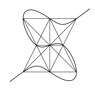
Figure 2: The configuration $012$, $034$, $056$, $078$, $135$, $147$, $168$, $238$ of level $8$ which contains two further collinearities when constrained on a cubic curve.

5 The Hilbert functions of the nine points

In the previous Section we classified points on an irreducible cubic curve, according to the possible collinearities. It is therefore quite natural to ask about the Hilbert functions of the ideal of the nine points of each configuration. First, observe that the linear system of nine points on an irreducible cubic curve has dimension either $0$ or $1$ (see [12] and [10]); hence, if $I$ is the ideal of the nine points $P_{0},\dots,P_{8}$, then $\dim\left(R/I\right)_{3}=9$ or $\dim\left(R/I)\right)_{3}=8$, where $R=K[x,y,z]$. Suppose $F\in R$ is the generic homogeneous polynomial of degree $d\geq 3$, with coefficients $a_{0},a_{1},\dots,a_{m-1}$, $m={d+2\choose d}$, and let $M(d,P)$ be the $9\times m$ matrix whose rows are the coefficients of $a_{0},a_{1},\dots$ in $F(P_{i})$ ($i=0,\dots,8$). The matrix $M(d,P)$ has rank at most $9$.

Lemma 10.

If $M(d,P)$ has rank $9$, then also $M(d+1,P)$ has rank $9$.

Proof..

We can assume that (after a change of coordinates, if necessary) all the points $P_{i}$ have the last coordinate different from zero and hence can be chosen equal to $1$. Let $F=a_{0}x^{d}+a_{1}x^{d-1}y+a_{2}x^{d-1}z+\cdots$, then the generic polynomial of degree $d+1$ can be seen as $F\cdot z+H(x,y)$, where $H$ is the generic homogeneous polynomial of degree $d+1$ in $x,y$. With these notations, the first $m$ columns of $M(d+1,P)$ are the matrix $M(d,P)$. From this, the result follows. ∎

This lemma allows to obtain the following:

Theorem 11.

The Hilbert function of $R/I$, where $I$ is the ideal of points of the configurations described in theorem 8 is either $0\mapsto 1,1\mapsto 3,2\mapsto 6,3\mapsto 9,4\mapsto 9,\dots$, if there exists only one irreducible cubic containing the points, or $0\mapsto 1,1\mapsto 3,2\mapsto 6,$ $3\mapsto 8,$ $4\mapsto 9,$ $5\mapsto 9,\dots$ in the other case, when the linear system of the cubic curves through the points is of dimension $1$.

Proof..

If the nine points are contained in only one cubic curve, the result immediately follows from lemma 10. If we have two irreducible cubic curves through the nine points, the result is a consequence of the fact that the points are a complete intersection. ∎

It is possible to verify that, when the level of a configuration is $5$ or more, only one of the two Hilbert functions is possible for that configuration, meanwhile, it can happen that a configuration of level $4$ or less admits both Hilbert functions:

Example 12.

Consider the configuration of level 4: $012,034,056,078$. In general, the linear system of $9$ points in this configuration is of dimension $0$ but there are suitable positions of the points which are contained in two irreducible cubic curves, like the following: $P_{0}=(0\!:0\!:1)$, $P_{1}=(1\!:0\!:1)$, $P_{2}=(2\!:0\!:1)$, $P_{3}=(0\!:1\!:1)$, $P_{4}=(0\!:2\!:1)$, $P_{5}=(2\!:-3\!:1)$, $P_{6}=(4\!:-6\!:-5)$, $P_{7}=(30\!:-19\!:9)$, $P_{8}=(60\!:-38\!:15)$.

References

-
[1]
J. Abbott, A. M. Bigatti, and L. Robbiano.
CoCoA: a system for doing Computations in Commutative
Algebra.
Available at
http://cocoa.dima.unige.it, 2019. - [2] M.C. Beltrametti, A. Logar, and M.L. Torrente. Complete intersection of cubic and quartic curves and a classification of the configurations of lines of quartic monoid surfaces, (2019). In preparation.
- [3] J. Bokowski and B. Sturmfels. Computational Synthetic Geometry. Springer-Verlag, 1989.
- [4] S.A. Burr, B. Grünbaum, and N.J.A. Sloane. The orchard problem. Geom. Dedicata, 2:397–424, 1974.
- [5] H.S.M. Coxeter. Self-dual configurations and regular graphs. Bull. Amer. Math. Soc., 56(5):413–455, 1950.
- [6] H.S.M. Coxeter. The pappus configuration and the self-inscribed octagon. i. Nederl. Akad. Wetensch. Proc. Ser. A, 80(4):256–269, 1977.
- [7] H.S.M. Coxeter. The pappus configuration and the self-inscribed octagon. ii. Nederl. Akad. Wetensch. Proc. Ser. A, 80(4):270–284, 1977.
- [8] H.S.M. Coxeter. The pappus configuration and the self-inscribed octagon. iii. Nederl. Akad. Wetensch. Proc. Ser. A, 80(4):285–300, 1977.
- [9] H. Cundy and C. Parry. Some cubic curves associated with a triangle. Journal of Geometry, 53:41–66, 1995.
- [10] L. Farnik. On computing the dimension of a system of planes curves. Univ. Iagel. Acta Math., 47:229–242, 2009.
- [11] W. Fulton. Algebraic Curves. Addison-Wesley, 1989.
- [12] A. V. Geramita, B. Harbourne, and J. Migliore. Classifying hilbert functions of fat point subschemes in . Collect. Math., 60(2):159–192, 2009.
- [13] B. Grünbaum. Configuration of points and lines. American Math. Soc., 2009.
- [14] W. McCune and R. Padmanabhan. Automated reasoning about cubic curves. Computers and Mathematics with Applications, 29(2):17–26, 1995.
- [15] W. McCune and R. Padmanabhan. Automated Deduction in Equational Logic and Cubic Curves. Lecture Notes in Computer Science. Springer-Verlag, 04 1996.
- [16] N.S. Mendelsohn, R. Padmanabhan, and Wolk B. Placement of the Desargues configuration on a cubic curve. Geom. Dedicata, 40:165–170, 1991.
- [17] E. Moorhouse. Incidence Geometry. University of Wyoming, 2007.
-
[18]
proofwiki.
Orchard planting problem.
https://proofwiki.org/wiki/Orchard_Planting_Problem, 2019. - [19] W.A. Stein et al. Sage Mathematics Software (Version 6.7). The Sage Development Team, 2019. http://www.sagemath.org.
- [20] Wikipedia The Free Encyclopedia. The Sylvester–Gallai theorem, available on the site. https://en.wikipedia.org/wiki/Sylvester-Gallai_theorem, 2019.