Prospects for single photon sideband cooling
in fermionic Lithium

Abstract

We present an analytic and numerical study for realizing single photon sideband cooling in an ultracold sample of fermionic Lithium trapped in a periodic optical potential. We develop an analytical model and obtain a master equation for the bound level populations. The cooling sequence is simulated both with a laser at a fixed frequency and with a frequency sweep. Finally, a Monte Carlo simulation is performed taking into account the full hyperfine spectrum of ^6Li. We find that a gas of ^6Li atoms loaded from a Magneto-Optical trap into a deep optical lattice can be cooled down to a $99\text{\,}\%$ occupancy of the lattice ground state after a $5\text{\,}\mathrm{ms}$ single photon sideband cooling using the D1 line of Li.

Introduction

Resolved sideband cooling (RSC) is a laser cooling technique used to cool trapped particles to their ground state of motion. RSC has been succesfully implemented in several experiments involving trapped ions[1] and ultracold atoms loaded in an optical lattice[2].

In order to introduce the working principle of RSC, let us consider the particle as a two-level system (TLS), with states $\ket{g}$, $\ket{e}$ and natural linewidth of the excited state $\gamma$. Let us also assume that the ground and the excited states perceive the same trapping potential and that the trapping potential is harmonic. In this model each state of the TLS is transformed in a manifold $\ket{i,n}$, where $i=g,e$ and where $n$ represents the quantum number of the motional state in the harmonic oscillator. RSC is a two-step process. In a first step the motional state of a trapped particle is changed by driving the $\ket{g,n}\to\ket{e,m}$ transition with a laser set at a frequency $\omega_{L}=\omega_{0}+(m-n)\omega_{T}$, where $\hbar\omega_{0}$ is the energy difference between ground and excited states in the TLS, while $\omega_{T}$ is the harmonic trap frequency. In the second step the particle internal state goes back to the $\ket{g}$ internal level, e.g. by spontaneous emission, but to a lower motional state with respect to the initial one. If the states of the TLS are long-lived states this second step of RSC is usually realized through optical pumping, as in Raman sideband cooling.

In order to be efficient, sideband cooling requires two conditions to be satisfied.
The first condition is that the motional level separation must be larger than the recoil energy associated with the laser absorption. This is quantified by the Lamb-Dicke parameter $\eta=k_{z}z_{0}$, where $k_{z}$ is the projection of the laser wavevector along the harmonic oscillator axis and $z_{0}$ is the spread of the zero-point harmonic wavefunction.
For implementing an efficient sideband cooling, the system must be in the Lamb-Dicke regime, i.e. $\eta\ll 1$. In this regime it is possible to expand the light-atom interaction operator in powers of $\eta$[3]: the terms of the series expansion represent sideband transitions associated with the loss or gain of one or more motional quanta. The transition that leaves the motional state unchanged ($\Delta n=0$) is referred to as the carrier transition, while the blue and red sidebands are the transitions associated with the gain or loss of a vibrational quanta ($\Delta n=\pm 1$), respectively.
The second requirement is for the system to be in the so-called strong coupling condition, i.e. $\nu_{\text{trap}}>\gamma$, which ensures that sidebands and carrier are well resolved spectroscopically, so that they can be separately addressed by using laser light[4]. Since the carrier transition is the most intense, spontaneous emission will occur mainly without changing the vibrational number. Therefore, it is possible to cool the system through the optical cycle: $\ket{g,n}\to\ket{e,n-1}\to\ket{g,n-1}$.

Usually, single photon sideband cooling is performed on trapped ions since deep trapping potentials can be conveniently created with electric fields, and narrow optical transitions are available in most of the elements that are used for ion trapping. In cold atoms experiments, instead, narrow optical transitions are often not at hand — with the exception of alkaline-earth and alkaline-earth-like atoms. Therefore, in order to resolve the sidebands, 2-photon Raman processes between hyperfine levels are usually employed (see Ref.[5] for an example of a recent work on Lithium).

In this work we investigate the possibility of performing single photon sideband cooling on the D1 transition of neutral fermionic Lithium atoms trapped in a periodic optical potential. Single photon sideband cooling has two main benefits with respect to Raman transitions: first, the experimental setup is simpler since only one laser is required for cooling; second, the transition rate is higher and the cooling process in principle faster. In our investigation, we start from a TLS in a non-harmonic trap with different potentials for ground and excited states, and study RSC by using an analytical and a kinetic Monte Carlo simulation[6]. We then extend our simulation to include the hyperfine levels (HFS) of Lithium atoms at low intensity magnetic fields.

Mathematical model

We consider a relatively high-finesse ($f\approx 17000$) cavity resonating at $903.4\text{\,}\mathrm{nm}$ for trapping ^6Li atoms. The resulting dipole potential can be made deep enough that the system satisfies the strong coupling condition and is in the Lamb-Dicke regime. If we consider a cavity input power of $100\text{\,}\mathrm{mW}$, the $\ce{{}^{2}S_{\frac{1}{2}}}$ and $\ce{{}^{2}P_{\frac{1}{2}}}$ levels experience a trapping potential of depth $26\text{\,}\mathrm{mK}$ and $22\text{\,}\mathrm{mK}$, respectively. The equivalent harmonic trapping frequencies are $\nu_{g}=$9.5\text{\,}\mathrm{MHz}$$ and $\nu_{e}=$8.7\text{\,}\mathrm{MHz}$$. However, the harmonic approximation works only for the lowest motional energy levels, and in the calculations reported in this work we considered for the energy of the bound levels the mean energy of the corresponding Bloch bands.

In such conditions the system has approximately 70 bound levels, although the actual number of motional levels is slightly different for the ground and the excited internal states. Therefore, there is a number of bound levels in the ground state potential that cannot be cooled via RSC because there is no counterpart in the exited state energy spectrum. Both the strong coupling and the Lamb-Dicke regime conditions are satisfied for $80\%$ of the bound energy levels. Since the separation between the levels is not constant, carrier and sidebands associated with a different starting level do not coincide in frequency but rather spread out over a wide frequency range. LABEL:fig:sb_detuning shows the excitation spectrum for different initial bound states, where the front-most curve represents the spectrum of a particle in the lowest motional state $n=0$.

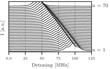
(a)

(b)

Figure 1:

The population of the different energy levels can be calculated analytically by building a master equation. To this end, we modify the model of Ref.s[3, 4] to include the dependence of the energy spectrum on the motional quantum number $n$, and find:

$$\begin{split}\dot{P}(n,t)&=(n+1)\ A_{-}(n+1)\ P(n+1)\\ &\quad+n\ A_{+}(n-1)\ P(n-1)\\ &\quad-[(n+1)A_{+}(n)\ +nA_{-}(n)]\ P(n)\,,\end{split}$$ (1)

where $A_{\pm}=\eta^{2}\quantity[\alpha\Gamma(\nu)+\Gamma(\nu-\nu_{n\to n\pm 1})]$ are the heating and cooling rates, $\nu_{n\to n\pm 1}$ is the difference in energy between the $n$-th and $(n\pm 1)$-th motional levels divided by the Planck constant, $\Gamma(\nu)$ is the scattering rate of the TLS for a laser of frequency $\nu$, $P(n)$ is the population of the n-th vibrational level, and $\alpha=\ifrac{2}{5}$ is an average angular factor in spontaneous emission.

One must also take into account the fact that the bound states $\ket{n}_{g}$ and $\ket{m}_{e}$, corresponding to motional levels of the ground and excited states, respectively, are not orthogonal, since they are associated to different trapping potentials. This non-orthogonality leads to an additional cooling and heating rate of the zero-th order in the Lamb-Dicke parameter[7]. We account for this effect by including the terms

$$R_{n\to m}=\absolutevalue{\innerproduct{e,m}{g,n}}^{2}\ \quantity[\alpha\Gamma(\nu)+\Gamma(\nu-\nu_{n\to m})]$$

in eq. 1. We approximate the value of the coefficients $\innerproduct{e,m}{g,n}$ by calculating the overlap integral between harmonic oscillator wavefunctions (an analytical expression can be found in Ref.[8]). Finally, we add a $A_{\pm}^{\text{trap}}$ in eq. 1 in order to consider the off-resonant scattering of light from the trapping laser, and we estimate a scattering rate of 5 photons per second.

In order to calculate the steady-state population of the different motional levels, we must solve the differential equation:

$$\dot{\overrightarrow{\mathbf{P}}}=\mathbf{A}\overrightarrow{\mathbf{P}}\,.$$

The population vector $\overrightarrow{\mathbf{P}}$ is defined by ${\{\overrightarrow{\mathbf{P}}\}}_{n}=P(n,t)$ and $\mathbf{A}$ is the coefficients matrix of the modified master equation, so that ${\{\mathbf{A}\}}_{n,m}$ represents the rate of transition between the states $\ket{n}_{g}$ and $\ket{m}_{g}$.
If the matrix $\mathbf{A}$ is time-independent a solution is given by

$$\overrightarrow{\mathbf{P}}=\sum_{i}c_{i}\overrightarrow{\mathbf{v}}_{i}e^{\lambda_{i}t}\,,$$ (2)

where $\overrightarrow{\mathbf{v}}_{i},\lambda_{i}$ are the eigenvectors and eigenvalues of the coefficient matrix, and $c_{i}$ are integration constants.

The solution of eq. 2 shows that the cooling with a laser at a fixed frequency is inefficient. Qualitatively, this is due to the fact that a laser resonant to the red sideband of the n-th level will scatter mainly photons in the blue sideband (and thus cause heating) of the k-th levels with $k>n$ (see LABEL:fig:sb_detuning). To solve this problem, we introduce in our model a frequency sweep of the sideband cooling laser. The laser light is initially tuned to the red sideband of a high energy bound level, and the frequency is then swept toward larger frequencies, in order to favour the cooling of lower energy levels. In this way the laser scans all the red sidebands from the most excited levels to the ground state, thus favouring the cooling of the largest possible number of atoms. In order to calculate the optimal frequency sweep for the cooling laser, we cannot use eq. 2, since the cooling and heating rates $A_{\pm}$ can not longer be considered constant. We solve this issue by discretizing time in time lags (of duration $\differential{t}=$1\text{\,}\mathrm{\SIUnitSymbolMicro s}$$) during which we assume $A_{\pm}$ to be constant. In this way, we solve eq. 2 iteratively over each time interval.

In order to calculate the initial distribution of the atoms in the optical potential’s bound states, we consider that the atoms are suddenly transferred from a magneto-optical trap (MOT) to the periodic potential. We assume that a single atom in the MOT is well approximated by a Gaussian wavepacket

$$\psi_{\sigma}(x)=\frac{1}{\sqrt{\sigma\sqrt{2\pi}}}\,e^{-\frac{x^{2}}{4\sigma^{2}}}\,e^{i\frac{p_{0}}{\hbar}x}$$

where $\sigma$ is the spatial extension of the wavepacket at $t=0$ and $p_{0}$ is the momentum associated with the group velocity of the wavepacket. We assume $\sigma=$500\text{\,}\mathrm{\SIUnitSymbolMicro m}$$ and $p_{0}=\sqrt{mk_{B}T_{0}}$, with $k_{B}$ the Boltzmann constant and $T_{0}=$40\text{\,}\mathrm{\SIUnitSymbolMicro K}$$ the initial temperature of the atoms[9]. The population of the n-th bound level is $P_{n}=c_{n}^{2}$, where:

$$c_{n}=\frac{1}{\sqrt{\sigma\sqrt{2\pi}}}\,\frac{1}{\sqrt{2^{n}n!\sqrt{\pi}}}\,\quantity(\frac{m\omega_{T}}{\hbar})^{1/4}\int_{-\infty}^{\infty}e^{-\quantity(\frac{m\omega_{T}}{2\hbar}+\frac{1}{4\sigma^{2}})x^{2}\,+\,i\frac{p_{0}}{\hbar}x}\,H_{n}\quantity(\sqrt{\frac{m\omega_{T}}{\hbar}}\,x)\$$

By substituting the Hermite polynomials $H_{n}(x)$ with the Gould-Hopper polynomials $H_{n}(x,y)$ using the relation $H_{n}(2x,-1)=H_{n}(x)$, the integral can be rewritten in a solvable form[8]. We calculate for our starting condition an initial average occupation number of $23$.

All calculations and simulations were performed by using a code written in Python and the open-source Scipy ecosystem[10]. The characteristic values of the Mathieu equation were also calculated numerically[11].

Results

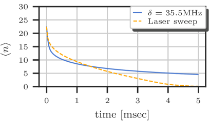
(a)

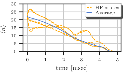
(b)

Figure 2:

LABEL:fig:cooling_TLS_result shows the average energy level as a function of the time in a simulated $5\text{\,}\mathrm{ms}$ cooling in the TLS approximation. We first simulate a cooling sequence with a fixed frequency laser and found that the initial average occupational number can be reduced by $\Delta n_{\%}=\ifrac{(n_{0}-n_{\text{fin}})}{n_{0}}=$79.6\text{\,}\%$$, where $n_{0}$ and $n_{\text{fin}}$ are the initial and final average occupation numbers, respectively, at an optimal detuning of $\delta=$35.5\text{\,}\mathrm{MHz}$$. This result slowly improves for times longer that $5\text{\,}\mathrm{ms}$, but only by a few percent. A considerably more efficient cooling is observed when using a laser sweep from $\delta_{0}=$26.2\text{\,}\mathrm{MHz}$$ to $\delta_{1}=$82.9\text{\,}\mathrm{MHz}$$: $\Delta n_{\%}=$99.3\text{\,}\%$$.

In order to include the HFS, one has to take into account the partial overlap between sidebands of different hyperfine levels of ^6Li. This may lead to the excitation of blue sidebands for some of the HFS. This effect can be compensated by using more than one laser frequency at the same time (see LABEL:fig:hfs_structure). One may still write a master equation for the full system, but the analytical solution would be affected by the round-off error arising in the diagonalization of a large coefficient matrix. Instead, we performed a kinetic Monte Carlo simulation of the master rate equation. The three required frequencies are swept together between the same detunings $\delta_{0}$ and $\delta_{1}$. LABEL:fig:cooling_full_result shows the result of the simulation, the motional number is reduced (in average over all HFS levels) by $\Delta n_{\%}=$99.9\text{\,}\%$$. All the calculations are valid for low homogeneous magnetic fields, up to 10 Gauss. For higher magnetic fields we observe that cooling is no longer efficient for some of the HF states, in particular when the magnetic field is increased over 20 Gauss.

The separation between red sidebands of two consecutive motional levels is on the order of $1\text{\,}\mathrm{MHz}$. It is therefore important to stabilize the trap depth in order to avoid a shift of the motional levels spectrum. We calculate that in order to maintain cooling efficiency above $95\text{\,}\%$ the laser power should be stabilized to a maximum $5\text{\,}\mathrm{mW}$ fluctuation, i.e. $\ifrac{\Delta P}{P_{0}}=$5\text{\,}\%$$, a value that can be achieved with a conventional stabilization of the laser power.

References

- [1] F. Diedrich, J.. Bergquist, Wayne M. Itano and D.. Wineland “Laser Cooling to the Zero-Point Energy of Motion” In Physical Review Letters 62.4 American Physical Society (APS), 1989, pp. 403–406 DOI: 10.1103/physrevlett.62.403
- [2] S.. Hamann et al. “Resolved-Sideband Raman Cooling to the Ground State of an Optical Lattice” In Physical Review Letters 80.19 American Physical Society (APS), 1998, pp. 4149–4152 DOI: 10.1103/physrevlett.80.4149
- [3] J. Javanainen and S. Stenholm “Laser cooling of trapped particles III: The Lamb-Dicke limit” In Applied Physics 24.2 Springer ScienceBusiness Media LLC, 1981, pp. 151–162 DOI: 10.1007/bf00902273
- [4] Stig Stenholm “The semiclassical theory of laser cooling” In Reviews of Modern Physics 58.3 American Physical Society (APS), 1986, pp. 699–739 DOI: 10.1103/revmodphys.58.699
- [5] Maxwell F. Parsons et al. “Site-Resolved Imaging of Fermionic \ce^6Li in an Optical Lattice” In Physical Review Letters 114.21 American Physical Society (APS), 2015 DOI: 10.1103/physrevlett.114.213002
- [6] Peter Kratzer “Monte Carlo and kinetic Monte Carlo methods” In ArXiv:0904.2556, 2009 arXiv:0904.2556 [cond-mat.mtrl-sci]
- [7] R. Taïeb et al. “Cooling and localization of atoms in laser-induced potential wells” In Physical Review A 49.6 American Physical Society (APS), 1994, pp. 4876–4887 DOI: 10.1103/physreva.49.4876
- [8] D. Babusci, G. Dattoli and M. Quattromini “On integrals involving Hermite polynomials” In ArXiv:1103.1210, 2011 arXiv:1103.1210 [math-ph]
- [9] A. Burchianti et al. “Efficient all-optical production of large\ce^6Li quantum gases using D1 gray-molasses cooling” In Physical Review A 90.4 American Physical Society (APS), 2014 DOI: 10.1103/physreva.90.043408
- [10] et al Virtanen P. “SciPy 1.0–Fundamental Algorithms for Scientific Computing in Python” In ArXiv:1907.10121, 2019 arXiv:1907.10121 [cs.MS]
- [11] Roberto Coisson, Graziano Vernizzi and Xiaoke Yang “Mathieu functions and numerical solutions of the Mathieu equation” In 2009 IEEE International Workshop on Open-source Software for Scientific Computation (OSSC) IEEE, 2009 DOI: 10.1109/ossc.2009.5416839