Adaptive Densely Connected Single Image Super-Resolution

Abstract

For a better performance in single image super-resolution(SISR), we present an image super-resolution algorithm based on adaptive dense connection (ADCSR). The algorithm is divided into two parts: BODY and SKIP. BODY improves the utilization of convolution features through adaptive dense connections. Also, we develop an adaptive sub-pixel reconstruction layer (AFSL) to reconstruct the features of the BODY output. We pre-trained SKIP to make BODY focus on high-frequency feature learning. The comparison of PSNR, SSIM, and visual effects verify the superiority of our method to the state-of-the-art algorithms.

1 Introduction

Single image super-resolution aims at reconstructing an accurate high-resolution image from the low-resolution image. Since deep learning made big progress in the computer version, many SISR algorithms based on deep Convolution Neural Networks (CNN) have been proposed in recent years. The powerful feature representation and end-to-end training skill of CNN makes a huge breakthrough in SISR.

Dong et al. [5] first proposed SRCNN by introducing a three-layer CNN for image SR. Kim et al. increased the number of layers to 20 in VDSR [10] and DRCN [11],making notable improvements over SRCNN. As we all know, the deeper the network is, the more powerful the representation it has. However, with the depth of network grow, gradient disappear and gradient explosion will be the main problem to hinder the performance of the network. This problem was solved when He et al. [6] proposed residual net (ResNet), and Huang et al. [7] proposed dense net (DesNet). Many large scale networks were introduced in SISR, such as SRResNet [14], EDSR [16], SRDenseNet [24], RDN [32] etc.These methods aim at building a deeper network to increase the performance. Other methods such as RCAN [31] and SAN [4] try to learn the correlation of the features in the middle layers.

WDSR [28] allows for better network performance with less computational effort. AWSRN [25] applies an adaptive weighted network. Weight adaptation is achieved by multiplying the residual convolution and the residual hopping by coefficients respectively, and the coefficients can be trained. Since the performance of dense connections is better than the residual [16] [32], we develop an adaptive densely connection method to enhance the efficiency of feature learning. There is a similar global SKIP, a single sub-pixel convolution, in WDSR [28]and AWSRN [25]. Although the SKIP is set to recover low-order frequencies, there is no practical measure to limit its training. We present an adaptive densely connected super-resolution reconstruction algorithm (ADCSR). The algorithm is divided into two parts: BODY and SKIP. BODY is focused on high-frequency information reconstruction through pre-training the SKIP. ADCSR obtained the optimal SISR performance based on bicubic interpolation. There are three main tasks:

(1)WDSR [4]is optimized using adaptive dense connections. Experiments were carried out by initializing the adaptive parameters and optimizing the models. Based on the above efforts, the performance of the network has been greatly improved;

(2)We propose the AFSL model to perform image SR through adaptive sub-pixel convolution;

(3)We develop a method which pre-train SKIP first and then train the entire network at the same time. Thus, the BODY is focused on the reconstruction of high-frequency details to improve network performance.

2 Related Works

SISR has important applications in many fields, such as security and surveillance imaging [33], medical imaging [21], and image generation [9]. The simplest method among them is the interpolation, such as linear interpolation, bicubic interpolation, and so on. This method takes the average of the pixel points in the known LR image as the missing pixel of the HR image. Interpolation works well in the smooth part of the image, but it works poorly in the edge regions, causing ringing and blurring. Additionally, learning-based and reconstruction-based methods are more complex such as sparse coding [27], neighborhood embedded regression [3] [23], random forest [19], etc.

Dong et al. first proposed a Convolutional Neural Network (CNN)-based super-resolution reconstruction network (SRCNN) [5], which performance is better than the most advanced algorithm at the time. Later, Shi et al. proposed a sub-pixel convolution super-resolution reconstruction network [20]. The network contains several convolutional layers to learn LR image features. Reconstruction is performed using the proposed sub-pixel convolutional layer. We can directly reconstruct the image utilizing the convolutional features from the deep convolutional network. Lim et al. proposed an enhanced depth residual network (EDSR) [16], which made a significant performance through the deeper network. Other deep network like RDN [32] and MemNet [22], are based on dense blocks. Some networks focus on feature correlations in channel dimension, such as RCAN [31]and SAN [4].

The WDSR [28]proposed by Yu et al. draws two conclusions. First, when the parameters and calculations are the same, the model with more features before the activation function has better performance. Second, weight normalization (WN layer) can improve the accuracy of the network. In WDSR, there is a broader channel before the activation function of each residual block. Wang et al. proposed an adaptive weighted super-resolution network(AWSRN) based on WDSR [28]. It designs a local fusion block for more efficient residual learning. Besides, an adaptive weighted multi-scale model is developed. The model is used to reconstruct features and has superior performance in methods with roughly equal parameters.

Cao et al. proposed an improved Deep Residual Network (IDRN) [2]. It makes simple and effective modifications to the structure of residual blocks and skip-connections. Besides, a new energy-aware training loss EA-Loss was proposed. And it employs lightweight networks to achieve fast and accurate results. The SR feedback network (SRFBN) [15] proposed by Li et al. applies the RNN with constraints to process feedback information and performs feature reuse.

The Deep Plug and Play SR Network (DPSR)  [29] proposed by Zhang et al. can process LR images with arbitrary fuzzy kernels. Zhang et al. [30] obtained real sensor data by optical zoom for model training. Xu et al. [26]generated training data by simulating the digital camera imaging process. Their experiments have shown that SR using raw data helps to restore fine detail and clear structure.

Figure 1: The architecture of our proposed Adaptive Densely Connected Super-Resolution Reconstruction (ADCSR).The top is ADCSR,the middle are ADRU and AFSL,the bottom is ADRB.

3 Our Model

3.1 Network Architecture

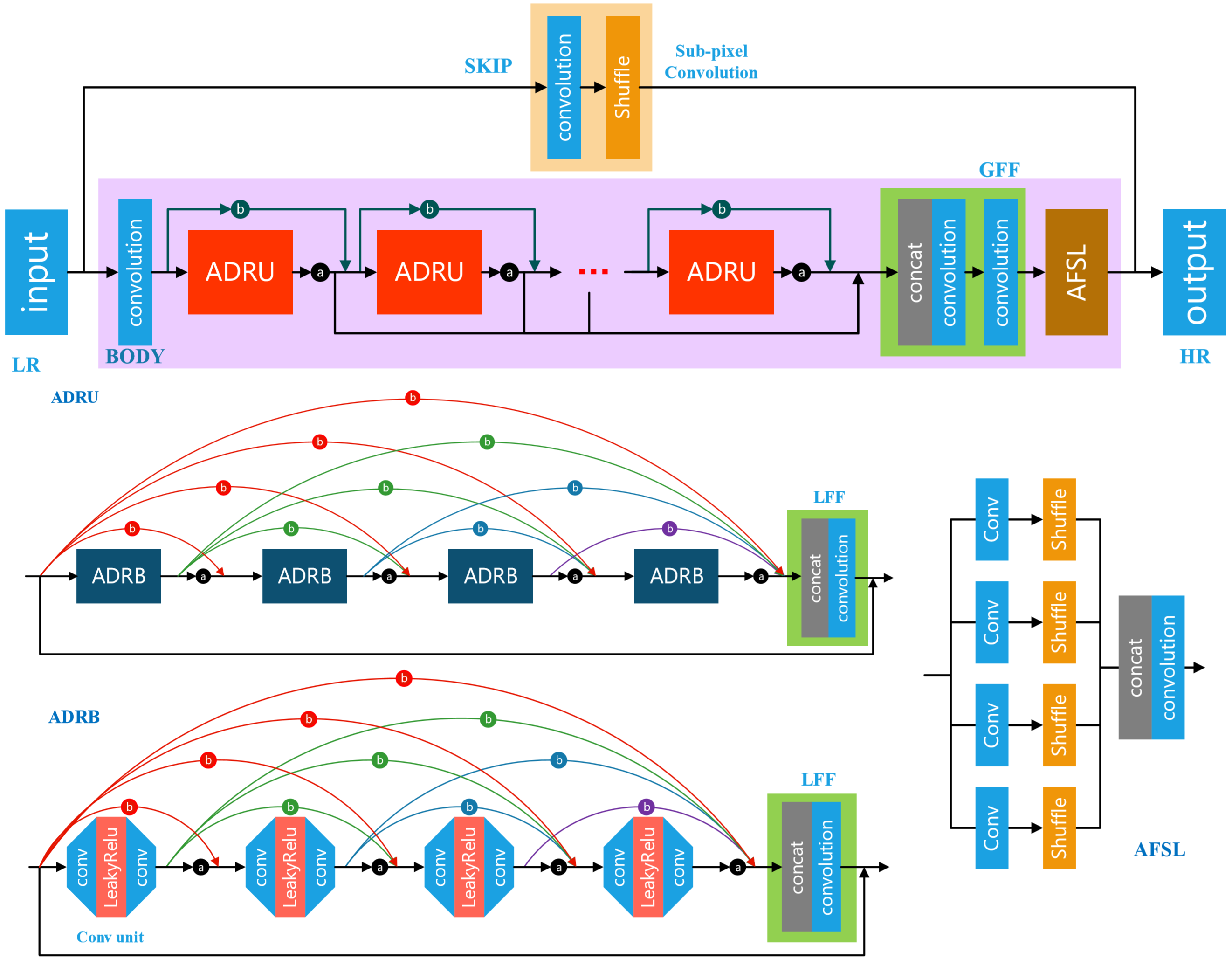
As shown in Figure 1, our ADCSR mainly consists two parts: SKIP and BODY. The SKIP just uses the sub-pixel convolution [20]. The BODY includes multiple ADRUs (adaptive, dense residual units), GFF (global feature fusion layer) [32], and an AFSL layer(adaptive feature sub-pixel reconstruction layer). The model takes the RGB patches from the LR image as input. On the one hand, the HR image is reconstructed by SKIP using the low-frequency information of the LR images. On the other hand, the image is reconstructed by BODY using the high-frequency information of the LR images. We can obtain the final complete reconstructed HR image by combining the results of SKIP and BODY.

SKIP consists of a single or multiple sub-pixel convolutions with a convolution kernel size of 5. we have:

$$HR_{SKIP}=f_{sub-conv5}(I_{LR})$$ (1)

where $HR_{SKIP}$ represents the output of skip part, $I_{LR}$ denotes the input image of LR and $f_{sub-conv5}$ represents the sub-pixel convolution, which convolution kernel size is 5.

In the BODY, first, we use a convolution layer to extract the shallow features from the LR image.

$$F_{f}=f_{conv3}(I_{LR})$$ (2)

where $f_{conv3}$ represents the feature extraction convolution, which kernel size is 3.

Second, we use several ADRUs to extract the deep features. There are four ADRBs (adaptive dense residual blocks) through adaptive dense connections in Each ADRU. The features are merged by the LFF (Local Feature Fusion Layer) and combined with a skip connection as the output of the ADRU. Each ADRB combines four convolution units by the same adaptive dense connection structure as ADRU. The convolution units adopt a convolution structure, which is similar to WDSR [28], including two layers of wide active convolution and one layer of Leakyrelu. After that, we fuse features by LFF, which combined with a skip connection as the output of the ADRB. GFF fuses the outputs of multiple ADRUs by means of concatenation and convolution.

$$X_{ADRUk+1}=b_{k}X_{ADRUk}+a_{k}f_{ADRUk}(X_{ADRUk})$$ (3)

where $X_{ADRUk}$ denotes the input feature map of $k$th ADRU, $f_{ADRUk}$ means the function of $k$th ADRU, $a_{k}$, $b_{k}$ are hyperparameters.

$$\begin{split}Y_{ADRUk}=&a_{k}f_{ADRUk}(X_{ADRUk})\\ Y_{ADRUlast}=&b_{last}X_{ADRUlast}+\\ &a_{last}f_{ADRUlast}(X_{ADRUlast})\end{split}$$ (4)

$Y_{ADRUk}$ means the output of the $k$th ADRU, and $Y_{ADRUlast}$ represents the output of the last ADRU, which includes the skip connection.

The third part of BODY uses the GEF to combine all the output of ADRU, which fuses features by two convotion layers.

$$\begin{split}F_{GFF}=f_{conv3}(f_{conv1}(&concat(Y_{ADRU1},\\ &...,Y_{ADRUn})))\end{split}$$ (5)

where $concat$ means feature fusion.

Finaly, Image upsampling via AFSL. The AFSL consists of four sub-pixel convolution branches of different scales with a convolution kernel size of 3, 5, 7, and 9, respectively. The output is obtained through the junction layer and a single layer convolution.

$$\begin{split}F_{AFSL}=f_{conv1}(&concat(f_{sub-conv3}(F_{GFF}),\\ &f_{sub-conv5}(F_{GFF}),\\ &f_{sub-conv7}(F_{GFF}),\\ &f_{sub-conv9}(F_{GFF})))\end{split}$$ (6)

In the second stage of BODY, the feature amplification layer is also implemented by a single convolution layer. The whole BODY is:

$$\begin{split}HR_{BODY}=F_{AFSL}((F_{GFF}(F_{f}(I_{LR}))))\end{split}$$ (7)

$HR_{BODY}$represents the output of BODY. The whole network can be expressed by formulas (8).

$$HR=HR_{BODY}+HR_{SKIP}$$ (8)

3.2 ADRB and ADRU

We will demonstrate the superiority of the adaptive dense connection structure in Chapter 4. To use as much adaptive residual structure as possible, we split the ADRU into ADRBs using adaptive dense connections and split ADRB into densely connected convolution units. At the same time, to get better results with less parameter amount, we use the residual block in WDSR as our convolution unit. As shown in Figure 1, ADRB and ADRU have similar connection structure. ADRB contains four convolution units, each of which can be represented by equotion (9).

$$f_{conv-unit}=f_{1conv3}(LeakyRelu(f_{2conv3}(x)))$$ (9)

where $x$ means the input of the convolution units. The kernel size of the $f_{1conv3}$ is $[3,3,feats,3\times feats]$, and the $f_{2conv3}$ is $[3,3,3\times feats,feats]$, $feat$ is the input channels of the convolution units.

The whole ADRB can be expressed by equation (10).

$$\begin{split}&Y_{1}=f_{conv\_unit1}(x)\\ &X_{1}=a_{01}(Y_{1})+b_{01}(x)\\ &Y_{2}=f_{conv\_unit2}(X_{1})\\ &X_{2}=a_{12}(Y_{2})+b_{12}(Y_{1})+b_{02}(x)\\ &Y_{3}=f_{conv\_unit3}(X_{2})\\ &X_{3}=a_{23}(Y_{3})+b_{23}(Y_{2})+b_{13}(Y_{1})+b_{03}(x)\\ &Y_{4}=f_{conv\_unit4}(X_{3})\\ &\begin{split}f_{ADRB}=f_{conv1}(&concat(a_{34}Y_{4},b_{34}Y_{3},\\ &b_{24}Y_{2},b_{14}Y_{1},b_{04}x))+x\end{split}\end{split}$$ (10)

where $f_{conv\_unit1}$means convolution unit, $x$ denotes the input of ADRB. $a_{mn},b_{mn}$ are hyperparameter, $X_{i}$ denotes the input of $(i+1)$th convolution unit, $Y_{j}$represents the output of $j$th convolution unit.

The whole ADRU can be formulated by equation (11).

$$\begin{split}&Y_{1}=f_{ADRB1}(x)\\ &X_{1}=a_{01}(Y_{1})+b_{01}(x)\\ &Y_{2}=f_{ADRB2}(X_{1})\\ &X_{2}=a_{12}(Y_{2})+b_{12}(Y_{1})+b_{02}(x)\\ &Y_{3}=f_{ADRB3}(X_{2})\\ &X_{3}=a_{23}(Y_{3})+b_{23}(Y_{2})+b_{13}(Y_{1})+b_{03}(x)\\ &Y_{4}=f_{ADRB4}(X_{3})\\ &\begin{split}f_{ADRU}=f_{conv1}(&concat(a_{34}Y_{4},b_{34}Y_{3},\\ &b_{24}Y_{2},b_{14}Y_{1},b_{04}x))+x\end{split}\end{split}$$ (11)

3.3 Implementation

In this section, we will give specific implementation details. In SKIP, the convolution channel for the sub-pixel convolutional layer is defined as 5. The convolution kernel size of the LFF in BODY is 1.The two convolution kernel sizes of GFF are 1 and 3, respectively. In AFSL, the convolution kernels are 3, 5, 7 and 9. All other convolution kernel sizes are set to 3. There are 4 ADRUs in BODY. The number of output channels in feature extraction layer, convolution unit, LFF, and GFF are 128, and the 4 sub-pixel convolutions and the final output in AFSL are 3. The stride size is 1 throughout the network while using Leakyrelu as the activation function.

4 Experiments

4.1 Adaptive dense connections

We propose a structure for adaptive dense connections such as ADRU, and verify its performance through experiments. In the experiment, we designed three models. The model parameters are the same, and the calculations are roughly equal. The structure of the models is similar to the ADCSR consisting of a single ADRU. These three models are:
a. Add LFF [32] on WDSR [4] (to obtain the same model depth);
b. Add a dense connection based on a;
c. Add parameter adaptation based on b.
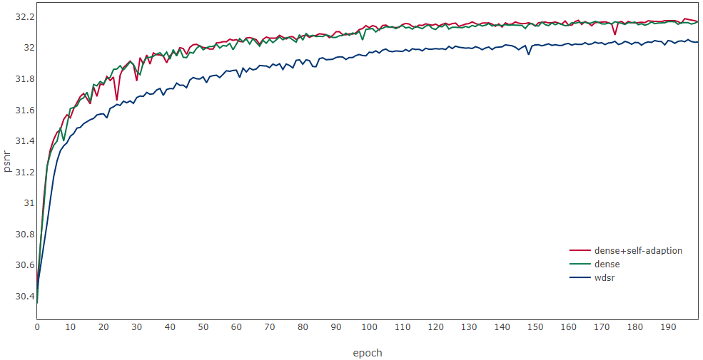
The three models have the same training parameters. We train our models with the data set DIV2K [16]. We also compare the performance on the standard benchmark dataset: B100 [17]. The number of iterations is 200. The learning rate is $1\times 10^{-4}$ and halved at every 100 epochs. As shown in Figure 2, networks with dense connections and parameter adaptation have the highest performance under the same conditions.

Figure 2: Convergence analysis of tests on B100 with scaling factor $\times 2$ during different model structures

4.2 Adaptive sub-pixel reconstruction layer (AFSL)

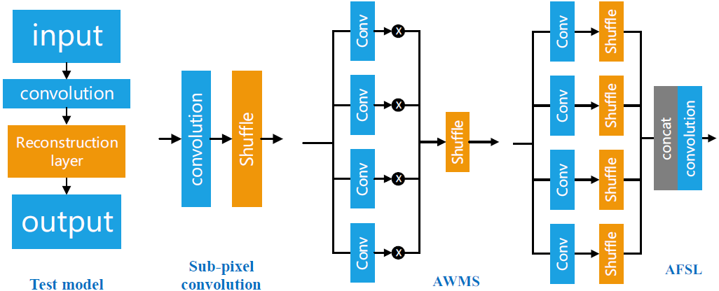
We test the reconstruction layer in BODY. We have designed a new reconstruction network model AFSL. To verify the performance of the model, we designed a straightforward model for comparison experiments. The model only includes the feature extraction layer and the reconstruction layer. As shown in Figure 3, the reconstruction layers are Sub-pixel convolution [20], AWMS [25], and AFSL. We performed the task on scale $\times 2$. The feature extraction layers and experimental parameters of the models are the same. We tested the models with B100 [17] and Urban100 [8]. At the same time, we also analyzed the difference in the number of FLOPs and model parameters. The result is shown in Table 1. We can see that AWMS and AFSL require more calculations and parameters than Sub-pixel convolution while its performance is better. In the case where the setting and the calculated amount are the same, the performance of AFSL is slightly better than AWMS.

Figure 3: Test model and structural Comparison of Three Reconstruction Layers

Table 1: Performance comparison of three reconstruction layers

	B100	Urban100	FLOPs	Params
Sub-conv	30.402	27.750	0.02G	9K
AWMS	30.590	27.956	0.30G	128K
AFSL	30.592	27.958	0.30G	128K

4.3 Pre-training SKIP

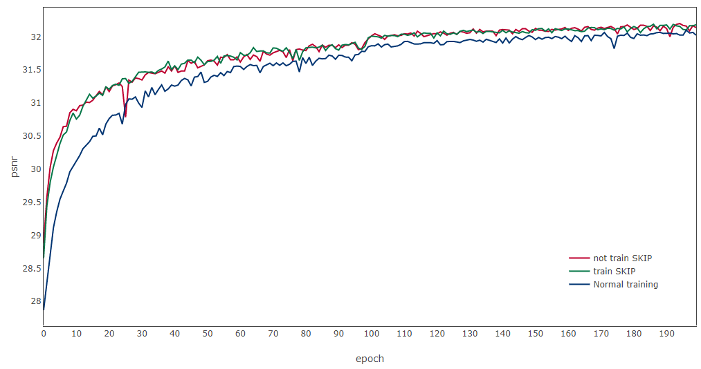
We have explored a training method that performs a separate pre-training of SKIP while training the entire model. This training method is used to make SKIP focus on the reconstruction of low-frequency information, while BODY focuses on high-frequency information reconstruction. We employ the same model, that is, the ADCSR containing a single ADRU with the same training parameters. But we train the model in different ways:
a. Train the entire network directly;
b. First pre-train SKIP, then train the whole network at the same time;
c. First pre-train SKIP, then set SKIP to be untrainable when training the entire network.

Figure 4 compares the image and image spectrum of SKIP and BODY output for models a and b. By comparing the output images, it can be seen that the BODY of the pre-trained SKIP model focuses on learning the texture edge details of the image. From the comparison of the output spectrum of the BODY part, the spectrogram of the pre-trained SKIP model is darker near the center and brighter around. It proves that the proposed method makes the BODY use more high-frequency information and less low-frequency information.

Figure 4: Results of pre-training SKIP on SKIP output

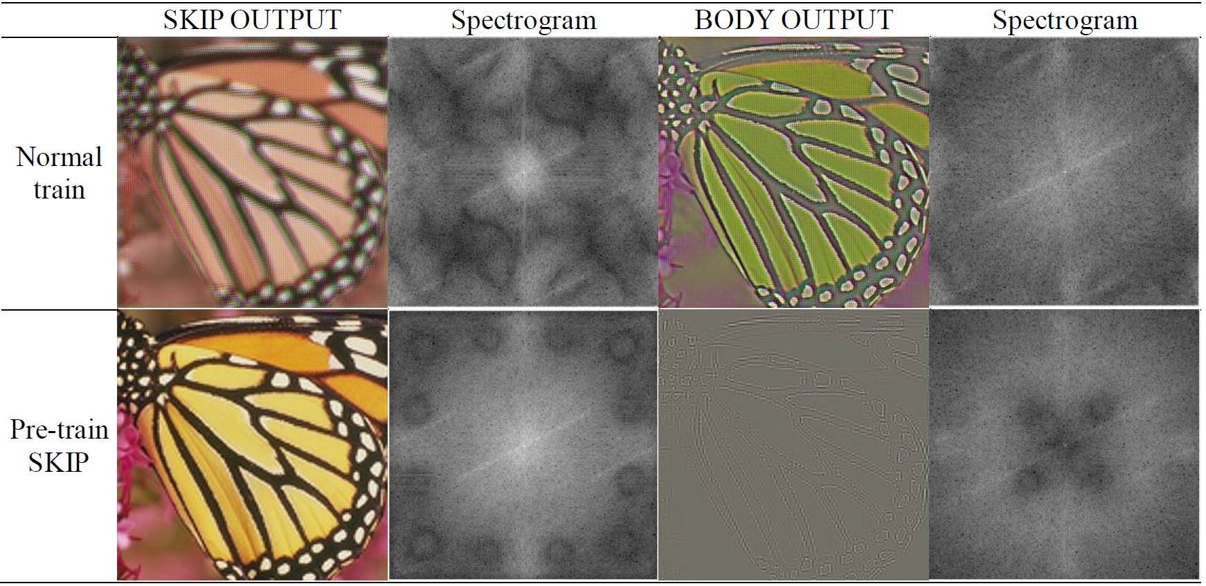
Figure 5 is a comparison of the test curves of the model on the B100 under different training modes. We found that networks that were pre-trained with SKIP achieved higher performance. And the network performance of tests b and c are similar.

Figure 5: Convergence analysis of tests on B100 with scaling factor $\times 2$ during different model training methods

4.4 Training settings

We train our network with dataset DIV2K and Flickr2K [16]. The training set has a total of 3,450 images without data augmentation. DIV2K is composed of 800 images for training while 100 images each for testing and validation. Flickr2K has 2,650 training images. The input image block size is $48\times 48$. SKIP is trained separately, and then the entire network is trained at the same time. The initial learning rate is $1\times 10^{-4}$. When the learning rate drops to $5\times 10^{-7}$, the training stops. we also adopt L1 loss to optimize our model. We train the network of scale $\times 2$ firstly. Subsequently, when training the network of scale $\times 3$, $\times 4$, the BODY parameter of the scale $\times 2$ is loaded (excluding the parameters of the AFSL). We train the model through the NVIDIA RTX2080Ti. Pytorch1.1.0+Cuda10.0+cudnn7.5.0 is selected as the deep learning environment.

Table 2: Quantitative evaluation of competing methods. We report the performance of state-of-the-art algorithms on widely used publicly available datasets, in terms of PSNR (in dB) and SSIM. The best results are highlighted with read color while the blue color represents the second-best SR.

method	scale	Set5 [1]		Set14 [27]		B100 [17]		Urban100 [8]		manga109 [18]
		PSNR	SSIM	PSNR	SSIM	PSNR	SSIM	PSNR	SSIM	PSNR	SSIM
Bicubic SRCNN [5] VDSR [10] LapSRN [12] MemNet [22] EDSR [16] RDN [32] RCAN [31] SAN [4] ADCSR ADCSR+	$\times 2$	33.66	0.9299	30.24	0.8688	29.56	0.8431	26.88	0.8403	30.80	0.9299
		36.33	0.9542	32.45	0.9067	31.36	0.8879	29.50	0.8946	35.60	0.9663
		37.53	0.9590	33.05	0.9130	31.90	0.8960	30.77	0.9140	37.22	0.9750
		37.52	0.9591	33.08	0.9130	31.08	0.8950	30.41	0.9101	37.27	0.9740
		37.78	0.9597	33.28	0.9142	32.08	0.8978	31.31	0.9195	37.72	0.9740
		38.11	0.9602	33.92	0.9195	32.32	0.9013	32.93	0.9351	39.10	0.9773
		38.24	0.9614	34.01	0.9212	32.34	0.9017	32.89	0.9353	39.18	0.9780
		38.27	0.9614	34.12	0.9216	32.41	0.9027	33.34	0.9384	39.44	0.9786
		38.31	0.9620	34.07	0.9213	32.42	0.9028	33.10	0.9370	39.32	0.9792
		38.33	0.9619	34.48	0.9250	32.47	0.9033	33.61	0.9410	39.84	0.9798
		38.38	0.9620	34.52	0.9252	32.50	0.9036	33.75	0.9418	39.97	0.9800
Bicubic SRCNN [5] VDSR [10] LapSRN [12] MemNet [22] EDSR [16] RDN [32] RCAN [31] SAN [4] ADCSR ADCSR+	$\times 3$	30.39	0.8682	27.55	0.7742	27.21	0.7385	24.46	0.7349	26.95	0.8556
		32.75	0.9090	29.30	0.8215	28.41	0.7863	26.24	0.7989	30.48	0.9117
		33.67	0.9210	29.78	0.8320	28.83	0.7990	27.14	0.8290	32.01	0.9340
		33.82	0.9227	29.87	0.8320	28.82	0.7980	27.07	0.8280	32.21	0.9350
		34.09	0.9248	30.00	0.8350	28.96	0.8001	27.56	0.8376	32.51	0.9369
		34.65	0.9280	30.52	0.8462	29.25	0.8093	28.80	0.8653	34.17	0.9403
		34.71	0.9296	30.57	0.8468	29.26	0.8093	28.80	0.8653	34.13	0.9484
		34.74	0.9255	30.65	0.8482	29.32	0.8111	29.09	0.8702	34.44	0.9499
		34.75	0.9300	30.59	0.8476	29.33	0.8112	28.93	0.8671	34.30	0.9494
		34.86	0.9305	30.81	0.8505	29.40	0.8127	29.44	0.8767	34.95	0.9521
		34.93	0.9310	30.88	0.8514	29.43	0.8133	29.57	0.8784	35.11	0.9528
Bicubic SRCNN [5] VDSR [10] LapSRN [12] MemNet [22] EDSR [16] RDN [32] RCAN [31] SAN [4] ADCSR ADCSR+	$\times 4$	28.42	0.8104	26.00	0.7027	25.96	0.6675	23.14	0.6577	24.89	0.7866
		30.45	0.8628	27.50	0.7513	26.90	0.7101	24.52	0.7221	27.58	0.8555
		31.35	0.8830	28.02	0.7680	27.29	0.7251	25.18	0.7540	28.83	0.8870
		31.54	0.8850	28.19	0.7720	27.32	0.7270	25.21	0.7560	29.09	0.8900
		31.74	0.8893	28.26	0.7723	27.40	0.7281	25.50	0.7630	29.42	0.8942
		32.46	0.8968	28.80	0.7876	27.71	0.7420	26.64	0.8033	31.02	0.9148
		32.47	0.8990	28.81	0.7871	27.72	0.7419	26.61	0.8028	31.00	0.9173
		32.63	0.9002	28.87	0.7889	27.77	0.7436	26.82	0.8087	30.40	0.9082
		32.64	0.9003	28.92	0.7888	27.78	0.7436	26.79	0.8068	31.18	0.9169
		32.77	0.9013	29.02	0.7917	27.86	0.7457	27.15	0.8174	31.76	0.9212
		32.82	0.9020	29.09	0.7930	27.90	0.7466	27.27	0.8197	31.98	0.9232

Figure 6: Visual results with bicubic degradation model($\times 4$) on Urban100

Figure 7: Two-stage adaptive dense connection super-resolution reconstruction network (DSSR)

4.5 Results with Bicubic Degradation

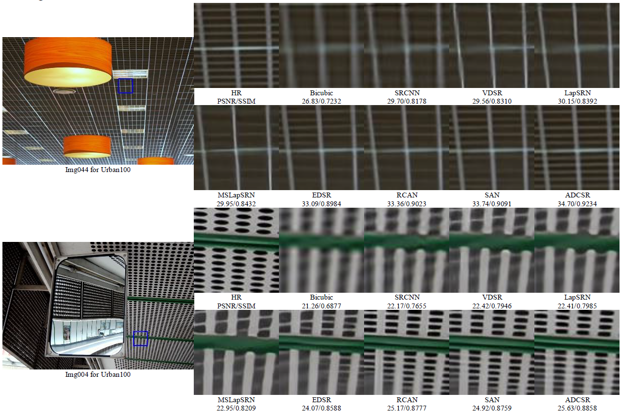
In order to verify the validity of the model , we compare the performance on five standard benchmark datasets: Set5 [1], Set14 [27], B100 [17], Urban100 [8], and manga109 [18]. In terms of PSNR, SSIM and visual effects, We compare our models with the state-of-the-art methods including Bicubic, SRCNN [5], VDSR [10], LapSRN [12], MemNet [22], EDSR [16], RDN [32], RCAN [31], SAN [4]. We also adopt self-ensemble strategy [16] to further improve our ADCSR and denote the self-ensembled ADCSR as ADCSR+. The results are shown in Table 2. As can be seen from the table, the PSNR and SSIM of the algorithm in $\times 2$, $\times 3$, $\times 4$ exceed the current state of the art.

Figure 6 show the Qualitative comparison of our models with Bicubic, SRCNN [5], VDSR [10], LapSRN [12], MSLapSRN [13], EDSR [16], RCAN [31], and SAN [4] . The images of SRCNN, EDSR, and RCAN are derived from the author’s open-source model and code. Test images for VDSR, LapSRN, MSLapSRN, SAN are provided by their respective authors. In the comparison chart of img044 in Figure 6, the image reconstructed by the algorithm is clear and close to the original image. In img004, our algorithm has a better visual effect.

5 AIM2019: Extreme Super-Resolution Challenge

This work is initially proposed for the purpose of participating in the AIM2019 Extreme Super-Resolution Challenge. The goal of the contest is to super-resolve an input image to an output image with a magnification factor $\times 16$ and the challenge is called extreme super-resolution.

Our model is the improved ADCSR, a two-stage adaptive dense connection super-resolution reconstruction network (DSSR). As shown in Figure 7, the DSSR consists of two parts, SKIP and BODY. The SKIP is a simple sub-pixel convolution [20]. The BODY part is divided into two stages. The first stage includes a feature extraction layer, multiple ADRUs (adaptive, dense residual units), GFF (global feature fusion layer) [32], and an AFSL layer (adaptive feature sub-pixel reconstruction layer).The second stage includes a feature amplification layer, an ADRB (adaptive dense residual block), and an AFSL.

During the training of DSSR, the network converges slowly due to the large network. We divide the network into two parts for training to speed up network convergence. When training DSSR, we first train the SKIP. The network ADCSR of scale is used as a pre-training parameter while training the entire network. At the same time, the feature extraction layer of the first level and each ADRU are set to be untrainable. During the period, GFF, AFSL and later second-level network parameters are trained at normal learning rates $1\times 10^{-4}$. Finally, we train the entire network when the learning rate is small. We train DSSR with dataset DIV8K. Other training settings are the same as ADCSR. Our model final result on the full resolution of the DIV8K test images is ($\times 16$) : PSNR = 26.79, SSIM = 0.7289.

6 Conclusions

We propose an adaptive densely connected super-resolution reconstruction algorithm (ADCSR). The algorithm is divided into two parts: BODY and SKIP. BODY improves the utilization of convolution features by adaptively dense connections. We also explore an adaptive sub-pixel reconstruction layer (AFSL) to reconstruct the features of the BODY output. We pre-train SKIP in advance so that the BODY focuses on high-frequency feature learning. Several comparative experiments demonstrate the effectiveness of the proposed improved method. On the standard datasets, the comparisons of PSNR, SSIM, and visual effects show that the proposed algorithm is superior to the state-of-the-art algorithms.

References

- [1] Marco Bevilacqua, Aline Roumy, Christine Guillemot, and Marie Line Alberi-Morel. Low-complexity single-image super-resolution based on nonnegative neighbor embedding. 2012.
- [2] Yanpeng Cao, Zewei He, Zhangyu Ye, Xin Li, Yanlong Cao, and Jiangxin Yang. Fast and accurate single image super-resolution via an energy-aware improved deep residual network. Signal Processing, 162:115–125, 2019.
- [3] Hong Chang, Dit-Yan Yeung, and Yimin Xiong. Super-resolution through neighbor embedding. In Proceedings of the 2004 IEEE Computer Society Conference on Computer Vision and Pattern Recognition, 2004. CVPR 2004., volume 1, pages I–I. IEEE, 2004.
- [4] Tao Dai, Jianrui Cai, Yongbing Zhang, Shu-Tao Xia, and Lei Zhang. Second-order attention network for single image super-resolution. In Proceedings of the IEEE Conference on Computer Vision and Pattern Recognition, pages 11065–11074, 2019.
- [5] Chao Dong, Chen Change Loy, Kaiming He, and Xiaoou Tang. Learning a deep convolutional network for image super-resolution. In European conference on computer vision, pages 184–199. Springer, 2014.
- [6] Kaiming He, Xiangyu Zhang, Shaoqing Ren, and Jian Sun. Deep residual learning for image recognition. In Proceedings of the IEEE conference on computer vision and pattern recognition, pages 770–778, 2016.
- [7] Gao Huang, Zhuang Liu, Laurens van der Maaten, and Kilian Q. Weinberger. Densely connected convolutional networks. In The IEEE Conference on Computer Vision and Pattern Recognition (CVPR), July 2017.
- [8] Jia-Bin Huang, Abhishek Singh, and Narendra Ahuja. Single image super-resolution from transformed self-exemplars. In Proceedings of the IEEE Conference on Computer Vision and Pattern Recognition, pages 5197–5206, 2015.
- [9] Tero Karras, Timo Aila, Samuli Laine, and Jaakko Lehtinen. Progressive growing of gans for improved quality, stability, and variation. arXiv preprint arXiv:1710.10196, 2017.
- [10] Jiwon Kim, Jung Kwon Lee, and Kyoung Mu Lee. Accurate image super-resolution using very deep convolutional networks. In Proceedings of the IEEE conference on computer vision and pattern recognition, pages 1646–1654, 2016.
- [11] Jiwon Kim, Jung Kwon Lee, and Kyoung Mu Lee. Deeply-recursive convolutional network for image super-resolution. In Proceedings of the IEEE conference on computer vision and pattern recognition, pages 1637–1645, 2016.
- [12] Wei-Sheng Lai, Jia-Bin Huang, Narendra Ahuja, and Ming-Hsuan Yang. Deep laplacian pyramid networks for fast and accurate super-resolution. In Proceedings of the IEEE conference on computer vision and pattern recognition, pages 624–632, 2017.
- [13] Wei-Sheng Lai, Jia-Bin Huang, Narendra Ahuja, and Ming-Hsuan Yang. Fast and accurate image super-resolution with deep laplacian pyramid networks. IEEE transactions on pattern analysis and machine intelligence, 2018.
- [14] Christian Ledig, Lucas Theis, Ferenc Huszár, Jose Caballero, Andrew Cunningham, Alejandro Acosta, Andrew Aitken, Alykhan Tejani, Johannes Totz, Zehan Wang, et al. Photo-realistic single image super-resolution using a generative adversarial network. In Proceedings of the IEEE conference on computer vision and pattern recognition, pages 4681–4690, 2017.
- [15] Zhen Li, Jinglei Yang, Zheng Liu, Xiaomin Yang, Gwanggil Jeon, and Wei Wu. Feedback network for image super-resolution. In Proceedings of the IEEE Conference on Computer Vision and Pattern Recognition, pages 3867–3876, 2019.
- [16] Bee Lim, Sanghyun Son, Heewon Kim, Seungjun Nah, and Kyoung Mu Lee. Enhanced deep residual networks for single image super-resolution. In Proceedings of the IEEE conference on computer vision and pattern recognition workshops, pages 136–144, 2017.
- [17] David Martin, Charless Fowlkes, Doron Tal, Jitendra Malik, et al. A database of human segmented natural images and its application to evaluating segmentation algorithms and measuring ecological statistics. Iccv Vancouver:, 2001.
- [18] Yusuke Matsui, Kota Ito, Yuji Aramaki, Azuma Fujimoto, Toru Ogawa, Toshihiko Yamasaki, and Kiyoharu Aizawa. Sketch-based manga retrieval using manga109 dataset. Multimedia Tools and Applications, 76(20):21811–21838, 2017.
- [19] Samuel Schulter, Christian Leistner, and Horst Bischof. Fast and accurate image upscaling with super-resolution forests. In Proceedings of the IEEE Conference on Computer Vision and Pattern Recognition, pages 3791–3799, 2015.
- [20] Wenzhe Shi, Jose Caballero, Ferenc Huszár, Johannes Totz, Andrew P Aitken, Rob Bishop, Daniel Rueckert, and Zehan Wang. Real-time single image and video super-resolution using an efficient sub-pixel convolutional neural network. In Proceedings of the IEEE conference on computer vision and pattern recognition, pages 1874–1883, 2016.
- [21] Wenzhe Shi, Jose Caballero, Christian Ledig, Xiahai Zhuang, Wenjia Bai, Kanwal Bhatia, Antonio M Simoes Monteiro de Marvao, Tim Dawes, Declan O’Regan, and Daniel Rueckert. Cardiac image super-resolution with global correspondence using multi-atlas patchmatch. In International Conference on Medical Image Computing and Computer-Assisted Intervention, pages 9–16. Springer, 2013.
- [22] Ying Tai, Jian Yang, Xiaoming Liu, and Chunyan Xu. Memnet: A persistent memory network for image restoration. In Proceedings of the IEEE international conference on computer vision, pages 4539–4547, 2017.
- [23] Radu Timofte, Vincent De Smet, and Luc Van Gool. Anchored neighborhood regression for fast example-based super-resolution. In Proceedings of the IEEE international conference on computer vision, pages 1920–1927, 2013.
- [24] Tong Tong, Gen Li, Xiejie Liu, and Qinquan Gao. Image super-resolution using dense skip connections. In Proceedings of the IEEE International Conference on Computer Vision, pages 4799–4807, 2017.
- [25] Chaofeng Wang, Zheng Li, and Jun Shi. Lightweight image super-resolution with adaptive weighted learning network. arXiv preprint arXiv:1904.02358, 2019.
- [26] Xiangyu Xu, Yongrui Ma, and Wenxiu Sun. Towards real scene super-resolution with raw images. In Proceedings of the IEEE Conference on Computer Vision and Pattern Recognition, pages 1723–1731, 2019.
- [27] Jianchao Yang, John Wright, Thomas S Huang, and Yi Ma. Image super-resolution via sparse representation. IEEE transactions on image processing, 19(11):2861–2873, 2010.
- [28] Jiahui Yu, Yuchen Fan, Jianchao Yang, Ning Xu, Zhaowen Wang, Xinchao Wang, and Thomas Huang. Wide activation for efficient and accurate image super-resolution. arXiv preprint arXiv:1808.08718, 2018.
- [29] Kai Zhang, Wangmeng Zuo, and Lei Zhang. Deep plug-and-play super-resolution for arbitrary blur kernels. In Proceedings of the IEEE Conference on Computer Vision and Pattern Recognition, pages 1671–1681, 2019.
- [30] Xuaner Zhang, Qifeng Chen, Ren Ng, and Vladlen Koltun. Zoom to learn, learn to zoom. In Proceedings of the IEEE Conference on Computer Vision and Pattern Recognition, pages 3762–3770, 2019.
- [31] Yulun Zhang, Kunpeng Li, Kai Li, Lichen Wang, Bineng Zhong, and Yun Fu. Image super-resolution using very deep residual channel attention networks. In Proceedings of the European Conference on Computer Vision (ECCV), pages 286–301, 2018.
- [32] Yulun Zhang, Yapeng Tian, Yu Kong, Bineng Zhong, and Yun Fu. Residual dense network for image super-resolution. In Proceedings of the IEEE Conference on Computer Vision and Pattern Recognition, pages 2472–2481, 2018.
- [33] Wilman WW Zou and Pong C Yuen. Very low resolution face recognition problem. IEEE Transactions on image processing, 21(1):327–340, 2011.