Optimized Age of Information Tail for Ultra-Reliable Low-Latency Communications in Vehicular Networks

Abstract

While the notion of age of information (AoI) has recently been proposed for analyzing ultra-reliable low-latency communications (URLLC), most of the existing works have focused on the average AoI measure. Designing a wireless network based on average AoI will fail to characterize the performance of URLLC systems, as it cannot account for extreme AoI events, occurring with very low probabilities. In contrast, this paper goes beyond the average AoI to improve URLLC in a vehicular communication network by characterizing and controlling the AoI tail distribution. In particular, the transmission power minimization problem is studied under stringent URLLC constraints in terms of probabilistic AoI for both deterministic and Markovian traffic arrivals. Accordingly, an efficient novel mapping between AoI and queue-related distributions is proposed. Subsequently, extreme value theory (EVT) and Lyapunov optimization techniques are adopted to formulate and solve the problem considering both long and short packets transmissions. Simulation results show over a two-fold improvement, in shortening the AoI distribution tail, versus a baseline that models the maximum queue length distribution, in addition to a tradeoff between arrival rate and AoI.

I Introduction

Vehicle-to-vehicle (V2V) communication will play an important role in next-generation (5G) mobile networks and is envisioned as one of the most promising enabler for intelligent transportation systems [2, 3, 4]. Typically, V2V safety applications (e.g., forward collision warning, blind spot/lane change warning, and adaptive cruise control) are known to be time-critical, as they rely on acquiring real-time status updates from individual vehicles. In this regard, the European telecommunications standards institute (ETSI) has standardized two types of safety messages: cooperative awareness messages (CAMs) and decentralized environmental notification messages (DENMs) [5]. One key challenge for delivering such critical and status update messages in V2V networks is how to provide ultra-reliable and low-latency vehicular communication links.

Indeed, achieving ultra-reliable low-latency communication represents one of the major challenges faced by 5G and vehicular networks [6]. In particular, a system design based on conventional average values (e.g., latency, rate, and queue length) is not adequate to capture the URLLC requirements, since averages often ignore the occurrence of extreme events (e.g., high latency events) that negatively impacts the overall performance. To overcome this challenge, one can resort to the robust framework of extreme value theory (EVT) which characterizes the probability distributions of extreme events, defined as the tail of the latency distribution or queue length [7]. Remarkably, the majority of the existing V2V literature focuses primarily on average performance metrics [8, 9, 10, 11], which is not sufficient in a URLLC setting. Only a handful of recent works have considered extreme values for vehicular networks [12, 13]. In particular, the work in [12] focuses on studying large delays in vehicular networks using EVT, via simulations using realistic mobility traces, without considering any analytical formulation. In [13], the authors study the problem of transmit power minimization subject to a new reliability measure in terms of maximal queue length among all vehicle pairs. Therein, EVT was utilized to characterize the distribution of maximal queue length over the network.

Since V2V safety applications are time-critical, the freshness of a vehicle’s status updates is of high importance along with the low-latency requirement [14, 15, 16]. A relevant metric in quantifying this freshness is the notion of age of information (AoI) proposed in [16]. AoI is defined as the time elapsed since the generation instant of the latest received status update at a destination. Optimizing the AoI is fundamentally different from delay or throughput optimization. In [16], the authors derive the minimum AoI at an optimal operating point that lies between the extremes of maximum throughput and minimum delay. Thus, providing quality-of-service (QoS) in terms of AoI is essential for any time-critical application and has attracted lots of research interest recently in various fields such as energy harvesting [19, 20], wireless networked control systems [15], and vehicular networks [16, 21, 22]. However, except for [15], these works focus on optimizing average AoI metrics. While interesting, a system design based on average AoI cannot enable the unique requirements of URLLC. Instead, the AoI distribution needs to be considered especially when dealing with time-critical V2V safety applications. Only a handful of works investigated the distribution of AoI, e.g.,[14, 15, 23], and [24]. In [14, 15] the authors argue that computing an exact expression for the AoI distribution may not always be feasible. Therefore, they opt for computing a bound on the tail of the AoI distribution and use that bound to formulate a tractable α-relaxed upper bound minimization problem (α-UBMP) to find an optimal sampling (i.e. arrival) rate that minimizes the AoI violation probability for a given age limit. In [23], the AoI distribution is obtained in terms of the Laplace-Stieltjes transform (LST) and is expressed in terms of the stationary distributions of the system delay and the peak AoI, where the peak AoI, proposed in [25, Def. 3], is another freshness metric used within the literature [25, 26, 27, 24]. Finally, in [24], the peak AoI violation probability is first characterized by deriving the probability generating function (PGF) of the peak age. Then the violation probability is obtained through a saddlepoint approximation. However, while interesting, these works do not consider controlling the tail of AoI violation distribution.

I-A Contributions

The main contribution of this paper is a novel framework that allow the control of the tail of AoI distribution in V2V communication networks, thus going beyond the conventional average-based AoI. In particular, our key goal is to enable vehicular user equipment (VUE) pairs to minimize their transmit power while ensuring stringent latency and reliability constraints based on a probabilistic AoI violation measure. To capture both periodic and stochastic arrivals, we consider two queuing systems, namely a D/G/1 and a M/G/1 queuing system. To this end, since the AoI metric is a receiver-side metric while the transmit power allocation occurs at the transmitter, we first derive a novel relationship between the probabilistic AoI and the queue length of each VUE for the D/G/1 system, and between the probabilistic AoI and the arrival rate of each VUE, for the M/G/1 system. Moreover, in order to constrain the exceedance over the imposed threshold, we use the fundamental concepts of EVT to characterize the tail, and the excess value of the vehicles’ queues and arrival rates, which are then incorporated as the statistical constraints within our transmission power minimization problem. Furthermore, it is assumed that a roadside unit (RSU) is used to cluster VUEs into disjoint groups in terms of their geographic locations, thus mitigating interference and reducing the signaling overhead between VUEs and the RSU. Since the objective function and constraints are represented in time-averaged and steady-state forms, Lyapunov stochastic optimization techniques [28] are leveraged by each VUE pair to locally optimize its transmission power subject to probabilistic AoI constraints. Knowing the instantaneous state realization, the Lyapunov optimization framework allows each VUE to optimize its transmission power in each time slot based on the observed random events without considering the queue length transition between the current and successive time slots. Moreover, the Lyapunov framework allows optimization of long-term performance metric while achieving network stability.

We further note that in V2V communication, the size of safety messages are typically small (e.g., [29] and [30]). In addition, due to the high mobility of V2V networks, the small time slot duration restricts the blocklength in each transmission. The finite blocklength transmission will hinder the vehicles to achieve the Shannon rate with an infinitesimal decoding error probability [31]. In this regard, incorporating the blocklength and decoding error probability, the authors in [32] have provided an approximated rate formula and shown a performance gap between the Shannon rate-based design and finite blocklength regime. As a result, the impact of short packets on V2V network performance should also be investigated.

Therefore, in addition to the system analysis based on the Shannon rate, we also study the power minimization problem considering the short packet transmission which, however, yields a non-convex optimization problem. To deal with this non-convexity, the convex-concave procedure (CCP) is used to solve the power minimization problem. Finally, simulation results corroborate the usefulness of EVT in characterizing the distribution of AoI. The results also show that the proposed approach yields over two-fold performance gains in AoI compared to two baselines: the first baseline’s scheme is concerned about the high-order statistics of the network-wide maximal queue length but oblivious of the AoI [13], while the second baseline does not take into account the URLLC design for taming the AoI tail. Our results also reveal an interesting tradeoff between the arrival rate of the status updates, and the average and worst AoI achieved by the network. Finally, the results show the existence of a blocklength at which the violation probability of AoI is minimized.

In a nutshell, the main contributions of this work are as follows.

• We derive and propose a novel relationship between the probabilistic AoI and the queue dynamics of each VUE for the D/G/1 system. (Lemma 1)

• We derive and propose a novel relationship between the probabilistic AoI and the queue dynamics of each VUE for the M/G/1 system. (Lemma 2,3)

• Utilizing those relationships, we propose a novel framework to minimize VUEs’ transmit power while ensuring the probabilistic AoI constraint in terms of the derived queue dynamics relation.

• We invoke EVT to characterize the violation probability and Lyapunov optimization to solve the problem.

• In the finite blocklength regime, the convex-concave procedure (CCP) is utilized to convexify the power minimization problem.

The rest of this paper is organized as follows. In Section II, the system model is described. The reliability constraints and the studied problems, for both deterministic and Markovian arrival cases, are presented in Section III, followed by the proposed AoI-aware resource allocation policy in Section IV. In Section V, numerical results are presented while conclusions are drawn in Section VI.

II System Model

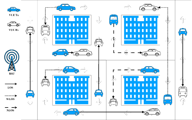
Figure 1: System and path loss models of the considered V2V network.

As shown in Fig. 1, we consider a V2V communication network based on a Manhattan mobility model [33], composed of a set $\mathcal{K}$ of $K$ VUE transmitter-receiver pairs under the coverage of a single RSU. During the entire communication lifetime, the association of each transmitter-receiver is assumed to be fixed. One potential application of this setup is to avoid the rear-end collision between vehicles, where the transmitter (e.g., vehicle in the front) sends a collision-warning message to the receiver (e.g., vehicle in the back) in a unicast manner [34, 35].

We consider a slotted communication timeline indexed by $t$, and the duration of each slot is denoted by $\tau$. Additionally, all VUE pairs share a set $\mathcal{N}$ of $N$ orthogonal resource blocks (RBs) with bandwidth $\omega$ per RB. We further denote the RB allocation as $\eta_{k}^{n}(t)\in\left\{0,1\right\},\forall k\in\mathcal{K},n\in\mathcal{N}$, where $\eta_{k}^{n}(t)=1$ indicates that RB $n$ is used by VUE pair $k$ in time slot $t$ and $\eta_{k}^{n}(t)=0$ otherwise. The transmitter of pair $k$ allocates a transmit power $P_{k}^{n}(t)\geq 0$ over RB $n$ to serve its receiver subject to a power constraint $\sum_{n\in\mathcal{N}}\eta_{k}^{n}(t)P_{k}^{n}(t)\leq P_{\textrm{max}}$, where $P_{\textrm{max}}$ is the total power budget per each VUE pair.

Let $h_{kk^{\prime}}^{n}(t)$ be the instantaneous channel gain, including path loss and channel fading, from the transmitter of pair $k$ to the receiver of pair $k^{\prime}$ over RB $n$ in slot $t$. We consider the $5.9\text{ GHz}$ carrier frequency and adopt the path loss model in [36]. For the path loss model, we have the line-of-sight (LOS), weak-line-of-sight (WLOS), and non-line-of-sight (NLOS) cases. Let us first denote an arbitrary transmitter’s and an arbitrary receiver’s Euclidean coordinates as $\boldsymbol{x}=(x_{1},x_{2})\in\mathbb{R}^{2}$ and $\boldsymbol{y}=(y_{1},y_{2})\in\mathbb{R}^{2}$, respectively. When the transmitter and receiver are on the same lane, we have an LOS path loss value as $l_{0}\left\|\boldsymbol{x}-\boldsymbol{y}\right\|^{-\alpha}$, where $\left\|.\right\|$ is the $l_{2}$-norm, $l_{0}$ is the path loss coefficient, and $\alpha$ is the path loss exponent. Additionally, when the transmitter and receiver are located separately on perpendicular lanes, we have the WLOS or NLOS case, depending on the transmitter and receiver’s locations. If, at least, one is near the intersection within a distance $\mathscr{D}$, we consider the WLOS path loss, i.e., $l_{0}\left\|\boldsymbol{x}-\boldsymbol{y}\right\|_{1}^{-\alpha}$ with the $l_{1}$-norm $\left\|.\right\|_{1}$. Otherwise, the NLOS case, with the path loss value $l_{0}^{{}^{\prime}}\left(|x_{1}-y_{1}|.|x_{2}-y_{2}|\right)^{-\alpha}$ and the path loss coefficient $l_{0}^{{}^{\prime}}<l_{0}\left(\frac{\mathscr{D}}{2}\right)^{\alpha}$, is considered. Fig. 1 illustrates these three path loss cases. The Shannon data rate of VUE pair $k$ in time slot $t$ (in the unit of packets per slot) is given by

$$R_{k}(t)=\frac{\omega\tau}{Z}{\textstyle\sum\limits_{n\in\mathcal{N}}}\log_{2}\left(1+\frac{P_{k}^{n}(t)h_{kk}^{n}(t)}{N_{0}\omega+I_{k}^{n}(t)}\right),$$ (1)

where $Z$ is the total packet size in bits which includes the payload of the packet as well as any headers/preambles, and $N_{0}$ is the power spectral density of the additive white Gaussian noise. Here, $I_{k}^{n}(t)=\sum_{k^{\prime}\in\mathcal{K}/k}\eta_{k^{\prime}}^{n}(t)P_{k^{\prime}}^{n}(t)h_{k^{\prime}k}^{n}(t)$ is the aggregate interference at the receiver of VUE pair $k$ over RB $n$ received from other VUE pairs operating over the same RB. We rely on a bit-pipe abstraction of the physical layer where bits are delivered reliably at a rate equal to (1).

Furthermore, each VUE transmitter has a queue buffer to store the data to be delivered to the desired receiver following a first-come first-serve (FCFS) policy. Denoting the VUE pair $k$’s queue length at the beginning of slot $t$ as $Q_{k}(t)$, the queue dynamics will be given by

$$Q_{k}(t+1)=\max\left(Q_{k}(t)-R_{k}(t),0\right)+A_{k}(t),$$ (2)

where $A_{k}(t)$ is the instantaneous packet arrival for VUE pair $k$ during slot $t$. In order to ensure queue stability, the following constraint needs to be satisfied

$$\lim_{C\to\infty}\frac{1}{C}{\textstyle\sum\limits_{t=0}^{C-1}}R_{k}(t)>\lambda\text{,}\leavevmode\nobreak\ \forall k\in\mathcal{K},$$ (3)

where $\lambda=\lim_{C\to\infty}\frac{1}{C}{\textstyle\sum\limits_{t=0}^{C-1}}A_{k}(t)$ is the average packet arrival rate per slot. Within this work, two arrival processes will be considered: 1) The deterministic arrival process, i.e., D/G/1, which account for the periodic nature of CAMs; 2) The Poisson arrival process, i.e., M/G/1, which accounts for the packet generation triggered by random events such as a hazard on the road. In the next section, the AoI-based reliability constrains are formulated for both cases.

III Enabling URLLC Based on Age of Information

Providing real-time status updates for mission critical applications is a key use case in V2V networks. These applications rely on the “freshness” of the data, which can be quantified by the concept of AoI [16]

$$\Delta_{k}(T)\triangleq T-\max_{i}\left(T_{k}^{\text{A}}\left(i\right)\mid T_{k}^{\text{D}}\left(i\right)\leq T\right).$$ (4)

Here, $\Delta_{k}(T)$ is the AoI of VUE pair $k$ at a time instant $T$. $T_{k}^{\text{A}}\left(i\right)$ and $T_{k}^{\text{D}}\left(i\right)$ represent the arrival and departure instants of packet $i$ of VUE pair $k$, respectively. As a reliability requirement, we impose a probabilistic constraint on the AoI for each VUE pair $k\in\mathcal{K}$, as follows:

$$\lim_{T\rightarrow\infty}\mathrm{Pr}\left\{\Delta_{k}(T)>d\right\}\leq\epsilon_{k}\text{, }\forall k\in\mathcal{K},$$ (5)

where $d$ is the age threshold, and $\epsilon_{k}\ll 1$ is the tolerable AoI violation probability. Consider an average arrival rate $\nicefrac{{\lambda}}{{\tau}}$ packets per second. The support of the steady state AoI distribution (and hence the existence of the limit in (5)) is $\left[\nicefrac{{\tau}}{{\lambda}},\infty\right)$ since AoI cannot be less than $\frac{\tau}{\lambda}$ with this given arrival rate [14]. To this end, since AoI is a receiver-side metric while the transmit power allocation occurs at the transmitter, a novel mapping between the AoI and the transmitter’s queue dynamics is proposed for both D/G/1 and M/G/1 cases.

III-A D/G/1 Queuing System (Deterministic Arrival)

In D/G/1 systems, arrivals are deterministic and periodic, as in the case of periodic CAMs in various V2V applications. Hence, the packet arrival rate per slot, $A_{k}(t)$, is constant and denoted by $A$, and the packet $i$’s arrival time instant will be $T_{k}^{\text{A}}\left(i\right)=\frac{i}{A}\tau$. Note that the indices of the packets that arrive during slot $t$ satisfy $i\in[tA,(t+1)A-1]$, while the packets that are served during the same slot will satisfy the following condition:

$$tA-Q_{k}(t)\leq i\leq tA-1-\max\left(Q_{k}(t)-R_{k}(t),0\right).$$ (6)

In [14], it is shown that for a given age limit $d_{\text{D}}$ with $\frac{A}{\tau}\geq\frac{1}{d_{\text{D}}}$, the steady state distribution of AoI for a D/G/1 queue can be characterized as

$$\lim_{T\rightarrow\infty}\mathrm{Pr}\Bigl{\{}\Delta_{k}(T)>d_{\text{D}}\Bigr{\}}=\lim_{T\rightarrow\infty}\mathrm{Pr}T_{k}^{\text{D}}({\color[rgb]{0,0,1}\hat{\imath}})>T,$$ (7)

where $\hat{\imath}\triangleq\lceil\frac{A}{\tau}(T-d_{\text{D}})\rceil$ is the index of the packet that first arrives at or after time $T-d_{\text{D}}$, and $d_{\text{D}}$ is the age threshold for the D/G/1 system. Next, in Lemma 1, we derive a mapping between the steady state distribution of the departure instant of a given packet and the queue length.

Lemma 1.

Given that $T$ is observed at the beginning of each slot $t+1$, i.e. $T=\tau(t+1)$, then

$$\mathrm{Pr}\left\{T_{k}^{\text{D}}(\hat{\imath})>\tau(t+1)\right\}\leq\mathrm{Pr}\left\{Q_{k}(t)>R_{k}(t)-\psi\right\},$$

where $\psi=2-(\frac{d_{\text{D}}}{\tau}-1)A$.

Proof:

See Appendix A. ∎

Combining (7) and Lemma 1, a sufficient condition for the probabilistic constraint (5) to hold in the slotted system can be written as

$$\lim_{C\to\infty}\frac{1}{C}{\textstyle\sum\limits_{t=0}^{C-1}}\mathrm{Pr}\left\{Q_{k}(t)>R_{k}(t)-\psi\right\}\leq\epsilon_{k}\text{, }\forall k\in\mathcal{K},$$ (8)

where the time average on $t$ represents the steady-state in the slotted system.

As previously mentioned, enabling URLLC requires the characterization of the tail of the AoI distribution. Therefore, we utilize the fundamental concepts of EVT [7] to investigate the event $Q_{k}(t)>R_{k}(t)-\psi$. The Pickands–Balkema–de Haan theorem for threshold violation of a random variable [7, Theorem 4.1] states that if a random variable $Q$ has a cumulative distribution function (CDF) denoted by $F_{Q}(q)$, and has a threshold value $\delta$. Then, as the threshold $\delta$ closely approaches $F_{Q}^{-1}(1)$, the conditional CDF of the excess value $X=Q-\delta>0$ denoted as $F_{X\text{|}Q>\delta}(x)=\mathrm{Pr}\left\{(Q-\delta)<x\rvert Q>\delta\right\}$, can be approximated by

$$G\left(x;\sigma,\xi\right)=\begin{cases}1-(\max\{1+\frac{\xi x}{\sigma},0\})^{-\frac{1}{\xi}},&\text{if }\xi\neq 0,\\ 1-e^{-\frac{x}{\sigma}},&\xi=0.\end{cases}$$

Here, $G\left(x;\sigma,\xi\right)$ is the generalized Pareto distribution (GPD) whose mean and variance are $\frac{\sigma}{1-\xi}$ and $\frac{\sigma^{2}}{(1-\xi)^{2}(1-2\xi)}$, respectively. Note that the value of the scale parameter $\sigma$ is threshold-dependent, except in the case when the shape parameter $\xi=0$ [7]. Also, note that a very low threshold $\delta$ is likely to violate the asymptotic basis of the model, leading to a bias; a very high threshold $\delta$ will generate few excesses with which the model can be estimated, leading to high variance [7]. Moreover, the characteristics of the GPD depend on the scale parameter $\sigma>0$ and the shape parameter $\xi<\frac{1}{2}$.

The Pickands–Balkema–de Haan theorem states that, for a sufficiently high threshold $\delta$, the distribution function of the excess value can be approximated by a GPD. In this regard, for (8), we define the conditional excess queue value of each VUE pair $k\in\mathcal{K}$ at time slot $t$ as $X_{k}^{\text{D}}(t)|_{Q_{k}(t)>R_{k}(t)-\psi}=Q_{k}(t)-R_{k}(t)+\psi$. Thus, we can approximate the mean and the variance of $X_{k}^{\text{D}}(t)$ as

$$\mathbb{E}\left[X_{k}^{\text{D}}(t)|Q_{k}(t)>R_{k}(t)-\psi\right] \approx\frac{\sigma_{k}}{1-\xi_{k}},$$ (9)

$$\text{Var}\left[X_{k}^{\text{D}}(t)|Q_{k}(t)>R_{k}(t)-\psi\right] \approx\frac{\sigma_{k}^{2}}{(1-\xi_{k})^{2}(1-2\xi_{k})},$$ (10)

with a scale parameter $\sigma_{k}$ and a shape parameter $\xi_{k}$. Note that the smaller the $\sigma_{k}$ and $\xi_{k}$, the smaller the mean value and variance of the GPD. Hence, in order to constraint the exceedance over the imposed threshold, we further impose thresholds on the scale and the shape parameters, i.e., $\sigma_{k}\leq\sigma_{k}^{\textrm{th}}$ and $\xi_{k}\leq\xi_{k}^{\textrm{th}}$ [38, 37]. Subsequently, applying both parameter thresholds and $\text{Var}\left(X_{k}^{\text{D}}\right)=\mathbb{E}\left[(X_{k}^{\text{D}})^{2}\right]-\mathbb{E}\left[X_{k}^{\text{D}}\right]^{2}$ to (9) and (10), we impose constraints for the time-averaged mean and second moment of the conditional excess queue value, i.e.,

$$\bar{X}_{k}^{\text{D}} =\lim_{C\rightarrow\infty}\frac{1}{C}{\textstyle\sum\limits_{t=0}^{C-1}}\mathbb{E}\left[X_{k}^{\text{D}}(t)\rvert Q_{k}(t)>R_{k}(t)-\psi\right]\leq H,$$ (11)

$$\bar{Y}_{k}^{\text{D}} =\lim_{C\rightarrow\infty}\frac{1}{C}{\textstyle\sum\limits_{t=0}^{C-1}}\mathbb{E}\left[Y_{k}^{\text{D}}(t)\rvert Q_{k}(t)>R_{k}(t)-\psi\right]\leq B,$$ (12)

where $H=\frac{\sigma_{k}^{\textrm{th}}}{1-\xi_{k}^{\textrm{th}}}$, $B=\frac{2(\sigma_{k}^{\textrm{th}})^{2}}{(1-\xi_{k}^{\textrm{th}})(1-2\xi_{k}^{\textrm{th}})}$ and $Y_{k}^{\text{D}}(t)\coloneqq\left[X_{k}^{\text{D}}(t)\right]^{2}$.

By denoting the RB and power allocation vectors as $\boldsymbol{\eta}(t)=\left[\eta_{k}^{n}(t)\right]_{k\in\mathcal{K}}^{n\in\mathcal{N}}$ and $\boldsymbol{P}(t)=\left[P_{k}^{n}(t)\right]_{k\in\mathcal{K}}^{n\in\mathcal{N}},\forall t$, respectively, the network-wide transmit power minimization problem is formulated as follows:

$$\mathbb{P}_{\text{D}}:\min_{\boldsymbol{\eta}(t),\boldsymbol{P}(t)} \leavevmode\nobreak\ \leavevmode\nobreak\ {\textstyle\sum\limits_{k\in\mathcal{K}}}{\textstyle\sum\limits_{n\in\mathcal{N}}}\bar{P}_{k}^{n}$$

s.t. $$\leavevmode\nobreak\ \leavevmode\nobreak\ \eqref{eq:queueStability_const},\eqref{eq:equiv_queue_constraint},\eqref{eq:GPDMean}\text{, and }\eqref{eq:GPD2moment},$$

$$\leavevmode\nobreak\ \leavevmode\nobreak\ {\textstyle\sum\limits_{n\in\mathcal{N}}}\eta_{k}^{n}(t)P_{k}^{n}(t)\leq P_{\textrm{max}},\leavevmode\nobreak\ \forall k\in\mathcal{K},$$ (13a)

$$\leavevmode\nobreak\ \leavevmode\nobreak\ 0\leq P_{k}^{n}(t)\leq P_{\textrm{max}},\text{ }\forall t,\,k\in\mathcal{K},\,n\in\mathcal{N},$$ (13b)

$$\leavevmode\nobreak\ \leavevmode\nobreak\ \eta_{k}^{n}(t)\in\{0,1\},\leavevmode\nobreak\ \forall t,\,k\in\mathcal{K},\,n\in\mathcal{N},$$ (13c)

where $\bar{P}_{k}^{n}=\lim\limits_{C\to\infty}\frac{1}{C}\sum_{t=0}^{C-1}P_{k}^{n}(t)$ is the time-averaged transmit power of VUE pair $k$ over RB $n$. In the following subsection, a similar problem is formulated and analyzed for the scenario considering the M/G/1 queuing system.

III-B M/G/1 Queuing System (Stochastic Arrival)

In M/G/1 systems, arrivals are Markovian (Poisson), which captures scenarios in which the packet generation in vehicles is triggered by a random event such as a road hazard, or sudden change in speed. Therefore, the probability of $I$ packet arrivals within the slot duration $\tau$ is

$$\mathrm{Pr}\left\{I\text{ packet arrivals within the slot duration }\tau\right\}=e^{-\lambda}\frac{\lambda^{I}}{I!},$$ (14)

where $\lambda$ is the average packet arrival rate per slot. In the following Lemma, we present a key insight regarding the steady state distribution of AoI for the M/G/1 queue, following similar procedures used in [14] for the D/G/1 case.

Lemma 2.

For an M/G/1 queuing system with an age threshold $d_{\text{M}}$ and $T<\infty$,

$$\mathrm{Pr}\left\{\Delta_{k}(T)>d_{\text{M}}\right\}=e^{-\frac{\lambda d_{\text{M}}}{\tau}}+\mathrm{Pr}T_{k}^{\text{D}}({\color[rgb]{0,0,1}\hat{\imath}})>T\left(1-e^{-\frac{\lambda d_{\text{M}}}{\tau}}\right),$$

where $\hat{\imath}$ is the index of the packet that first arrives at or after time $T-d_{\text{M}}$, and $d_{\text{M}}$ is the age threshold for the M/G/1 system.

Proof:

See Appendix B. ∎

Next, in Lemma 3 we propose a mapping between the steady state distribution of $T_{k}^{\text{D}}(\hat{\imath})$ and the arrival rate $A_{k}(t)$.

Lemma 3.

Given that $T$ is observed at the beginning of each slot $t$, i.e. $T=\tau t$, then

$$\mathrm{Pr}\left\{T_{k}^{\text{D}}(\hat{\imath})>T\right\}=\mathrm{Pr}\left\{A_{k}(t)>R_{k}(t)\right\}.$$

Proof:

See Appendix C. ∎

Combining the results of Lemma 2 and 3, the probabilistic constraint (5) can be rewritten as,

$$\lim_{C\to\infty}\frac{1}{C}{\textstyle\sum\limits_{t=0}^{C-1}}\mathrm{Pr}\left\{A_{k}(t)>R_{k}(t)\right\}\leq E_{k}\text{, }\forall k\in\mathcal{K},$$ (15)

where $E_{k}=\frac{\epsilon_{k}-e^{-\frac{\lambda d_{\text{M}}}{\tau}}}{1-e^{-\frac{\lambda d_{\text{M}}}{\tau}}}$, and $d_{\text{M}}\geq-\frac{\tau\ln\epsilon_{k}}{\lambda}$ to ensure $E_{k}\geq 0$. Similar to the previous subsection, we investigate the event $A_{k}(t)>R_{k}(t)$ and study the tail behavior of AoI using the Pickands–Balkema–de Haan theorem for threshold violation [7]. This yields two constraints for the time-averaged mean and second moment of the conditional excess value, as follows:

$$\bar{X}_{k}^{\text{M}} =\lim_{C\rightarrow\infty}\frac{1}{C}{\textstyle\sum\limits_{t=0}^{C-1}}\mathbb{E}\left[X_{k}^{\text{M}}(t)\rvert A_{k}(t)>R_{k}(t)\right]\leq H,$$ (16)

$$\bar{Y}_{k}^{\text{M}} =\lim_{C\rightarrow\infty}\frac{1}{C}{\textstyle\sum\limits_{t=0}^{C-1}}\mathbb{E}\left[Y_{k}^{\text{M}}(t)\rvert A_{k}(t)>R_{k}(t)\right]\leq B,$$ (17)

where $X_{k}^{\text{M}}(t)|_{A_{k}(t)>R_{k}(t)}=A_{k}(t)-R_{k}(t)$, and $Y_{k}^{\text{M}}(t)\coloneqq\left[X_{k}^{\text{M}}(t)\right]^{2}$. In this regard, the network wide transmit power minimization problem for the M/G/1 case is given by

$$\mathbb{P}_{\text{M}}:\min_{\boldsymbol{\eta}(t),\boldsymbol{P}(t)} \leavevmode\nobreak\ \leavevmode\nobreak\ {\textstyle\sum\limits_{k\in\mathcal{K}}}{\textstyle\sum\limits_{n\in\mathcal{N}}}\bar{P}_{k}^{n}$$

s.t. $$\leavevmode\nobreak\ \leavevmode\nobreak\ \eqref{eq:queueStability_const},\eqref{eq:PowerConst_1},\eqref{eq:PowerConst_2},\eqref{eq:RBConst},\eqref{eq:equiv_Constraint_MG1},\eqref{eq:GPDMean-MG1},\text{ and }\eqref{eq:GPD2moment-MG1}.$$

IV AoI-Aware Resource Allocation Using Lyapunov Optimization

Since the objective function and the constrains are represented in a time-average and steady-state forms, and in order to find the optimal resource $\boldsymbol{\eta}(t)$ and power $\boldsymbol{P}(t)$ allocation vectors of both deterministic and Markovian arrivals corresponding to problems $\mathbb{P}_{\text{D}}$ and $\mathbb{P}_{\text{M}}$, we invoke techniques from Lyapunov stochastic optimization [28]. Later on, we will study the impact of short packets and their effect on the problem formulation.

IV-A Deterministic Arrivals

To solve $\mathbb{P}_{\text{D}}$, we first rewrite the probabilistic constraint in (8) as a time-averaged constraint, so it could be utilized by the Lyapunov stochastic optimization, as follows:

$$\lim_{C\rightarrow\infty}\frac{1}{C}{\textstyle\sum\limits_{t=0}^{C-1}}R_{k}(t)\mathbbm{1}\left\{Q_{k}(t)>R_{k}(t)-\psi\right\}\leq\bar{\epsilon}_{k},$$ (19)

where $\bar{\epsilon}_{k}=\lim_{C\rightarrow\infty}\frac{1}{C}\sum_{t=0}^{C-1}R_{k}(t)\epsilon_{k}$ is the product of the time-averaged rate and the tolerance value $\epsilon_{k}$, and $\mathbbm{1}\left\{.\right\}$ is the indicator function. Using Lyapunov optimization, the time-averaged constraints (11), (12), (3), and (19) can be satisfied by converting them into virtual queues and maintain their stability [28], i.e. the lower bound of these constraints are considered as the arrival rate to the virtual queue, while the upper bounds are considered as its service rate. In this regard, we introduce the corresponding virtual queues with the dynamics shown in (20)–(23).

$$J_{k}^{(X)}(t+1) =\max\left(J_{k}^{(X)}(t)+(X_{k}^{\text{D}}(t)-H)\mathbbm{1}\left\{Q_{k}(t)>R_{k}(t)-\psi\right\},0\right),$$ (20)

$$J_{k}^{(Y)}(t+1) =\max\left(J_{k}^{(Y)}(t)+(Y_{k}^{\text{D}}(t)-B)\mathbbm{1}\left\{Q_{k}(t)>R_{k}(t)-\psi\right\},0\right),$$ (21)

$$J_{k}^{(R)}(t+1) =\max\left(J_{k}^{(R)}(t)-R_{k}(t)+A,0\right),$$ (22)

$$J_{k}^{(Q)}(t+1) =\max\left(J_{k}^{(Q)}(t)+R_{k}(t)\mathbbm{1}\left\{Q_{k}(t)>R_{k}(t)-\psi\right\}-R_{k}(t)\epsilon_{k},0\right).$$ (23)

 

For notation simplicity, let $\boldsymbol{J}(t)=\bigl{[}J_{k}^{(X)}(t),J_{k}^{(Y)}(t),J_{k}^{(Q)}(t),J_{k}^{(R)}(t),Q_{k}(t):k\in\mathcal{K}\bigr{]}$ denotes the combined physical and virtual queues vector. Then, in order to maintain the stability of $\boldsymbol{J}(t)$, we use the conditional Lyapunov drift-plus-penalty for time slot $t$, which can be expressed as

$$\mathbb{E}\biggl{[}\mathscr{L}\left(\boldsymbol{J}(t+1)\right)-\mathscr{L}\left(\boldsymbol{J}(t)\right)+\sum_{k\in\mathcal{K}}\sum_{n\in\mathcal{N}}VP_{k}^{n}(t)\rvert\boldsymbol{J}(t)\biggr{]},$$ (24)

where $\mathscr{L}\left(\boldsymbol{J}(t)\right)=\frac{\boldsymbol{J^{\text{T}}}(t)\boldsymbol{J}(t)}{2}$ is the Lyapunov function with $\boldsymbol{J^{\text{T}}}(t)$ being the transpose of $\boldsymbol{J}(t)$, and $V\geq 0$ is a parameter that controls the tradeoff between optimal transmit power and queue stability. By calculating the Lyapunov drift and leveraging the fact that $\left(\max\left(a-b,0\right)+c\right)^{2}\leq a^{2}+b^{2}+c^{2}-2a(b-c)\text{, }\forall a,b,c\geq 0$, and $\left(\max\left(x,0\right)\right)^{2}\leq x^{2}$, on (2) and (20)–(23), an upper bound on (24) can be obtained as

$$\eqref{eq:Lyapunov_drift} \leq\mathfrak{C}^{\text{D}}+\mathbb{E}\Biggl{[}\sum_{k\in\mathcal{K}}\biggl{(}\Bigl{(}J_{k}^{(Q)}(t)-J_{k}^{(X)}(t)-2\left(Q_{k}(t)+\psi\right)^{3}$$

$$-\left(2J_{k}^{(Y)}(t)+1\right)\left(Q_{k}(t)+\psi\right)\Bigr{)}\cdot\mathbbm{1}\left\{Q_{k}(t)>R_{k}(t)-\psi\right\}$$

$$-\left(J_{k}^{(R)}(t)+A+Q_{k}(t)+J_{k}^{(Q)}(t)\cdot\epsilon_{k}\right)\biggr{)}R_{k}(t)$$

$$+\sum_{k\in\mathcal{K}}\sum_{n\in\mathcal{N}}VP_{k}^{n}(t)\rvert\boldsymbol{J}(t)\Biggr{]}.$$ (25)

Here, $\mathfrak{C}^{\text{D}}=A^{2}+\left(J_{k}^{(R)}(t)+Q_{k}(t)\right)A+\left(1+\frac{1}{2}\epsilon_{k}^{2}\right)R_{k}^{2}(t)+\biggl{(}\frac{1}{2}\left(\left(Q_{k}(t)+\psi\right)^{4}+H^{2}+B^{2}\right)+\left(Q_{k}(t)+\psi\right)^{2}\left(\frac{1}{2}-B+J_{k}^{(Y)}(t)\right)+\left(Q_{k}(t)+\psi\right)\left(J_{k}^{(X)}(t)-H\right)-J_{k}^{(X)}(t)H-J_{k}^{(Y)}(t)B+\Bigl{(}H+2B\left(Q_{k}(t)+\psi\right)\Bigr{)}R_{k}(t)+\Bigl{(}1+3\left(Q_{k}(t)+\psi\right)^{2}-B+J_{k}^{(Y)}(t)-\epsilon_{k}\Bigr{)}R_{k}^{2}(t)-2\left(Q_{k}(t)+\psi\right)R_{k}^{3}(t)+\frac{1}{2}R_{k}^{4}(t)\biggr{)}\cdot\mathbbm{1}\left\{Q_{k}(t)>R_{k}(t)-\psi\right\}$ is a bounded term that does not affect the system performance. Note that the solution to problem $\mathbb{P}_{\text{D}}$ can be obtained by minimizing the upper bound in (25) in each slot $t$ [28], i.e.,

$$\hat{\mathbb{P}}_{\text{D}}:\min_{\boldsymbol{\eta}(t),\mathbf{P}(t)} {\textstyle\sum\limits_{k\in\mathcal{K}}}\Biggl{[}{\textstyle\sum\limits_{n\in\mathcal{N}}}VP_{k}^{n}(t)-\biggl{[}J_{k}^{(R)}(t)+A+Q_{k}(t)$$

$$+J_{k}^{(Q)}(t)\cdot\epsilon_{k}+\Bigl{(}-J_{k}^{(Q)}(t)+J_{k}^{(X)}(t)$$

$$+(2J_{k}^{(Y)}(t)+1)(Q_{k}(t)+\psi)+2(Q_{k}(t)+\psi)^{3}\Bigr{)}$$

$$\cdot\mathbbm{1}\left\{Q_{k}(t)>R_{k}(t)-\psi\right\}\biggr{]}R_{k}(t)\Biggr{]}$$

s.t. $$\eqref{eq:PowerConst_1}\text{-}\eqref{eq:RBConst}.$$

IV-B Markovian Arrivals

To solve $\mathbb{P}_{\text{M}}$, we first rewrite (15) as

$$\lim_{C\rightarrow\infty}\frac{1}{C}{\textstyle\sum\limits_{t=0}^{C-1}}R_{k}(t)\mathbbm{1}\left\{A_{k}(t)>R_{k}(t)\right\}\leq\bar{E}_{k},$$ (26)

where $\bar{E}_{k}=\lim_{C\rightarrow\infty}\frac{1}{C}\sum_{t=0}^{C-1}R_{k}(t)E_{k}$. Following the same procedures as in Section IV-A, the time-averaged constraints (16), (17), (3), and (26) are converted into virtual queues with the dynamics shown in (27)–(30).

$$M_{k}^{(X)}(t+1) =\max\left(M_{k}^{(X)}(t)+(X_{k}^{\text{M}}(t)-H)\mathbbm{1}\left\{A_{k}(t)>R_{k}(t)\right\},0\right),$$ (27)

$$M_{k}^{(Y)}(t+1) =\max\left(M_{k}^{(Y)}(t)+(Y_{k}^{\text{M}}(t)-B)\mathbbm{1}\left\{A_{k}(t)>R_{k}(t)\right\},0\right),$$ (28)

$$M_{k}^{(R)}(t+1) =\max\left(M_{k}^{(R)}(t)-R_{k}(t)+A_{k}(t),0\right),$$ (29)

$$M_{k}^{(Q)}(t+1) =\max\left(M_{k}^{(Q)}(t)+R_{k}(t)\mathbbm{1}\left\{A_{k}(t)>R_{k}(t)\right\}-R_{k}(t)E_{k},0\right).$$ (30)

 

Denoting $\boldsymbol{M}(t)=\bigl{[}M_{k}^{(X)}(t),M_{k}^{(Y)}(t),M_{k}^{(Q)}(t),M_{k}^{(R)}(t),Q_{k}(t):k\in\mathcal{K}\bigr{]}$ as the combined physical and virtual queue vector, the conditional Lyapunov drift-plus-penalty for slot $t$ is given by

$$\mathbb{E}\biggl{[}\mathscr{L}\left(\boldsymbol{M}(t+1)\right)-\mathscr{L}\left(\boldsymbol{M}(t)\right)+\sum_{k\in\mathcal{K}}\sum_{n\in\mathcal{N}}VP_{k}^{n}(t)\rvert\boldsymbol{M}(t)\biggr{]}.$$ (31)

By calculating the Lyapunov drift and leveraging the fact that $\left(\max\left(a-b,0\right)+c\right)^{2}\leq a^{2}+b^{2}+c^{2}-2a(b-c)\text{, }\forall a,b,c\geq 0$, and $\left(\max\left(x,0\right)\right)^{2}\leq x^{2}$, on (2) and (27)–(30), an upper bound on $\eqref{eq:Lyapunov_drift-MG1}$ can be obtained as follows:

$$\eqref{eq:Lyapunov_drift-MG1} \leq\mathfrak{C}^{\text{M}}+\mathbb{E}\Biggl{[}\sum_{k\in\mathcal{K}}\biggl{(}\Bigl{(}M_{k}^{(Q)}(t)-M_{k}^{(X)}(t)-2A_{k}^{3}(t)$$

$$-\left(2M_{k}^{(Y)}(t)+1\right)A_{k}(t)\Bigr{)}\cdot\mathbbm{1}\left\{A_{k}(t)>R_{k}(t)\right\}$$

$$-\left(M_{k}^{(R)}(t)+A_{k}(t)+Q_{k}(t)+M_{k}^{(Q)}(t)\cdot E_{k}\right)\biggr{)}R_{k}(t)$$

$$+\sum_{k\in\mathcal{K}}\sum_{n\in\mathcal{N}}VP_{k}^{n}(t)\rvert\boldsymbol{M}(t)\Biggr{]}.$$ (32)

Here, $\mathfrak{C}^{\text{M}}=\frac{1}{2}\left(A_{k}^{2}(t)+A_{k}(t)\right)+\Bigl{(}M_{k}^{(R)}(t)+Q_{k}(t)\Bigr{)}A_{k}(t)+\left(1+\frac{1}{2}E_{k}^{2}\right)R_{k}^{2}(t)+\biggl{(}\frac{1}{2}\left(A_{k}^{4}(t)+H^{2}+B^{2}\right)+A_{k}^{2}(t)\left(\frac{1}{2}-B+M_{k}^{(Y)}(t)\right)+A_{k}(t)\left(M_{k}^{(X)}(t)-H\right)-M_{k}^{(X)}(t)H-M_{k}^{(Y)}(t)B+\Bigl{(}H+2BA_{k}(t)\Bigr{)}R_{k}(t)+\Bigl{(}1+3A_{k}^{2}(t)-B+M_{k}^{(Y)}(t)-E_{k}\Bigr{)}R_{k}^{2}(t)-2A_{k}(t)R_{k}^{3}(t)+\frac{1}{2}R_{k}^{4}(t)\biggr{)}\cdot\mathbbm{1}\left\{A_{k}(t)>R_{k}(t)\right\}$ is a bounded term that does not affect the system performance. The solution to problem $\mathbb{P}_{\text{M}}$ can be obtained by minimizing the upper bound in (32) in each slot $t$ [28], i.e.,

$$\hat{\mathbb{P}}_{\text{M}}:\min_{\boldsymbol{\eta}(t),\mathbf{P}(t)} {\textstyle\sum\limits_{k\in\mathcal{K}}}\Biggl{[}{\textstyle\sum\limits_{n\in\mathcal{N}}}VP_{k}^{n}(t)-\biggl{[}M_{k}^{(R)}(t)+A_{k}(t)+Q_{k}(t)$$

$$+M_{k}^{(Q)}(t).E_{k}+\Bigl{(}-M_{k}^{(Q)}(t)+M_{k}^{(X)}(t)$$

$$+(2M_{k}^{(Y)}(t)+1)A_{k}(t)+2A_{k}^{3}(t)\Bigr{)}$$

$$\cdot\mathbbm{1}\left\{A_{k}(t)>R_{k}(t)\right\}\biggr{]}R_{k}(t)\Biggr{]}$$

s.t. $$\eqref{eq:PowerConst_1}\text{--}\eqref{eq:RBConst}.$$

To solve $\hat{\mathbb{P}}_{\text{D}}$ and $\hat{\mathbb{P}}_{\text{M}}$ each time slot $t$, the RSU needs full global channel state information (CSI) and queue state information (QSI). This is clearly impractical for vehicular networks since frequently exchanging fast-varying local information between the RSU and VUEs can yield a significant unacceptable overhead. To alleviate the information exchange burden, we utilize a two-timescale resource allocation mechanism which is performed in two stages. Therein, RBs for each VUE pair are centrally allocated over a long timescale at the RSU whereas each VUE pair minimizes its transmit power over a short timescale. In the next subsection, a more about the two-stage resource allocation mechanism is presented.

IV-C Two-Stage Resource Allocation

IV-C1 Spectral Clustering and RB Allocation at the RSU

It can be noted that the co-channel transmission of nearby VUE pairs can lead to severe interference. In order to avoid the interference from nearby VUEs, the RSU first clusters VUE pairs into $g>1$ disjoint groups, in which the nearby VUE pairs are allocated to the same group, and then the RSU orthogonally allocates all RBs to the VUE pairs in each group. Vehicle clustering is done by means of spectral clustering due to its ease of implementation and its efficient solvability by standard linear algebra methods [39]. We adopt the VUE clustering and RB allocation technique as in [13], denoting $\boldsymbol{v}_{k}\in\mathbb{R}^{2}$ as the Euclidean coordinate of the midpoint of VUE transmitter-receiver pairs $k$. Here, we use a distance-based Gaussian similarity matrix $\boldsymbol{F}$ to represent the geographic proximity information, in which the $(k,k^{\prime})$-th element is defined as

$$f_{kk^{\prime}}\coloneqq\begin{cases}e^{-\left\|\boldsymbol{v}_{k}-\boldsymbol{v}_{k^{\prime}}\right\|^{2}/\gamma^{2}},&\left\|\boldsymbol{v}_{k}-\boldsymbol{v}_{k^{\prime}}\right\|\leq\phi,\\ 0,&\text{otherwise},\end{cases}$$

where $\phi$ captures the neighborhood size, while $\gamma$ controls the impact of the neighborhood size. Subsequently, $\boldsymbol{F}$ is used to group VUE pairs using spectral clustering as shown in Algorithm 1. The most expensive step, in terms of computational complexity, within Algorithm 1 is the computation of the eigenvalues/eigenvectors of $\boldsymbol{I}-\boldsymbol{D}^{-\frac{1}{2}}\boldsymbol{F}\boldsymbol{D}^{-\frac{1}{2}}$ (step 3) which has a complexity $\mathcal{O}\left(K^{3}\right)$. The overall computational complexity of Algorithm 1 is $\mathcal{O}\left(K^{3}\right)$ [40]. Note that, the number of VUE pairs $K$ under the coverage of a single RSU is typically small. Hence, the computational complexity of the proposed solution will be reasonable in practice.

1:  Inputs: the Euclidean coordinate $\boldsymbol{v}_{k}$ of each VUE pair $k$, and the number of groups $g$.

2:  Calculate matrix $\boldsymbol{F}$ and the diagonal matrix $\boldsymbol{D}$ with the diagonal $d_{j}=\sum_{q=1}^{K}f_{jq}$.

3:  Let $\boldsymbol{U}=\left[\boldsymbol{u}_{1},\cdots,\boldsymbol{u}_{g}\right]$ in which $\boldsymbol{u}_{g}$ is the eigenvector of the $g$-th smallest eigenvalue of $\boldsymbol{I}-\boldsymbol{D}^{-\frac{1}{2}}\boldsymbol{F}\boldsymbol{D}^{-\frac{1}{2}}$.

4:  Use $k$-means clustering approach to cluster $K$ normalized row vectors (which represent $K$ VUE pairs) of matrix $\boldsymbol{U}$ into $g$ groups.

5:  Output: $K$ VUE pairs distributed among $g$ groups.

Algorithm 1 Spectral Clustering for VUE Grouping

After forming the groups, the RSU orthogonally allocates RBs to the VUEs inside the group. Hereafter, we denote $\mathcal{N}_{k}$ as the set of RBs that are allocated for VUE pair $k\in\mathcal{K}$. Moreover, to reduce the signaling overhead due to frequent information exchange between the RSU and VUE pairs, it is assumed that VUE clustering and RB allocation are performed in a longer time scale, i.e., every $T_{0}\gg 1$ time slots since the vehicles’ geographic location do not change significantly during the slot duration $\tau$ (i.e., coherence time of fading channels). Therefore, VUE pairs send their locations to the RSU only once every $T_{0}$ slots instead of every slot.

IV-C2 Transmit Power Allocation at the VUE

Since VUE pair $k$ can only use the set $\mathcal{N}_{k}$ of allocated RBs for the communication, we modify the power allocation and RB usage constraints, i.e., (13a)–(13c), $\forall k\in\mathcal{K}$, as

$$\begin{cases}\sum\limits_{n\in\mathcal{N}_{k}}P_{k}^{n}(t)\leq P_{\textrm{max}},\leavevmode\nobreak\ \forall t,\\ P_{k}^{n}(t)\geq 0,\leavevmode\nobreak\ \forall t,\,n\in\mathcal{N}_{k},\\ P_{k}^{n}(t)=0,\leavevmode\nobreak\ \forall t,\,n\notin\mathcal{N}_{k}.\end{cases}$$ (33)

Note that the RBs in $\mathcal{N}_{k}$ are reused by VUE transmitters in different groups. For tractability, we approximately treat the aggregate interference as a constant term $I_{0}$ and rewrite the transmission rate in (1) as

$$R_{k}(t)\approx\frac{\omega\tau}{Z}{\textstyle\sum\limits_{n\in\mathcal{N}_{k}}}\log_{2}\left(1+\frac{P_{k}^{n}(t)h_{kk}^{n}(t)}{N_{0}\omega+I_{0}}\right).$$ (34)

Subsequently, applying (33) and (34) to $\hat{\mathbb{P}}_{\text{D}}$ and $\hat{\mathbb{P}}_{\text{M}}$, the VUE transmitter of each VUE pair $k$ locally allocates its transmit power by solving the following convex optimization problem $\mathbb{P}_{1}$ in each slot $t$

$$\mathbb{P}_{1}:\min_{P_{k}^{n}(t)} \leavevmode\nobreak\ \leavevmode\nobreak\ {\textstyle\sum\limits_{n\in\mathcal{N}_{k}}}VP_{k}^{n}(t)-\Im_{k}(t)\log_{2}\left(1+\frac{P_{k}^{n}(t)h_{kk}^{n}(t)}{N_{0}\omega+I_{0}}\right)$$

subject to $$\leavevmode\nobreak\ \leavevmode\nobreak\ \eqref{eq:PowerConst_3},$$

where for $\hat{\mathbb{P}}_{\text{D}}$ that represents the D/G/1 system, $\Im_{k}(t)=\frac{\tau\omega}{Z}\Bigl{[}J_{k}^{(R)}(t)+A+Q_{k}(t)+J_{k}^{(Q)}(t)\epsilon_{k}+\bigl{(}-J_{k}^{(Q)}(t)+J_{k}^{(X)}(t)+(2J_{k}^{(Y)}(t)+1)(Q_{k}(t)+\psi)+2(Q_{k}(t)+\psi)^{3}\bigr{)}\cdot\mathbbm{1}\left\{Q_{k}(t)>R_{k}(t)-\psi\right\}\Bigr{]}$, while for $\hat{\mathbb{P}}_{\text{M}}$ that represents the M/G/1 system, $\Im_{k}(t)=\frac{\tau\omega}{Z}\Bigl{[}M_{k}^{(R)}(t)+A_{k}(t)+Q_{k}(t)+M_{k}^{(Q)}(t)E_{k}+\bigl{(}-M_{k}^{(Q)}(t)+M_{k}^{(X)}(t)+(2M_{k}^{(Y)}(t)+1)A_{k}(t)+2A_{k}^{3}(t)\bigr{)}\cdot\mathbbm{1}\left\{A_{k}(t)>R_{k}(t)\right\}\Bigr{]}$. Based on the Karush-Kuhn-Tucker (KKT) conditions, the optimal VUE transmit power $P_{k}^{n*}(t),\forall n\in\mathcal{N}_{k},$ of $\mathbb{P}_{1}$ satisfies

$$\frac{\Im_{k}(t)h_{kk}^{n}(t)}{(N_{0}\omega+I_{0}+P_{k}^{n*}(t)h_{kk}^{n}(t))\ln 2}=V+\zeta,$$

if $\frac{\Im_{k}(t)h_{kk}^{n}(t)}{(N_{0}\omega+I_{0})\ln 2}>V+\zeta.$ Otherwise, $P_{k}^{n*}(t)=0.$ Moreover, the Lagrange multiplier $\zeta$ is $0$ if $\sum_{n\in\mathcal{N}_{k}}P_{k}^{n*}(t)<P_{\textrm{max}}$, and we have $\sum_{n\in\mathcal{N}_{k}}P_{k}^{n}(t)=P_{\textrm{max}}$ when $\zeta>0$ . Note that, given a small value of $V$, the derived power $P_{k}^{n*}(t)$ provides a sub-optimal solution to problems $\mathbb{P}_{\text{D}}$ and $\mathbb{P}_{\text{M}}$, whose optimal solution is asymptotically obtained by increasing $V$.

IV-D Impact of Finite Blocklength

Due to the high mobility feature in V2V networks, the small time slot duration $\tau$ restricts the blocklength in each transmission. This obstructs vehicles from achieving the Shannon rate $\eqref{eq:rate_2}$ with an infinitesimal decoding error probability [32]. In consequence, the ultra-low packet loss probability cannot be ensured. Hence, depending on the Shannon rate $\eqref{eq:rate_2}$ may be optimistic for designing and optimizing V2V networks. According to [41], finite blocklength performance can be characterized by several techniques. one possibility is to fix the transmission rate and study the exponential decay of the error probability as the blocklength grows. This technique is referred to as “error exponent analysis”. An alternative analysis of the finite blocklength performance follows from fixing the decoding error probability and studying the maximum transmission rate as a function of the blocklength. This technique is referred to as “normal approximation” [32]. Taking into account this practical concern in finite blocklength transmission and following the normal approximation approach, the transmission rate $R_{k}(t)$ (in the unit of packet per slot) can be reformulated as [32]

$$R_{k}(t)=\frac{\omega\tau}{Z}{\textstyle\sum\limits_{n\in\mathcal{N}_{k}}}\biggl{(}\log_{2}\left(1+\rho_{k}\right)-\sqrt{\frac{\nu_{k}}{L}}Q^{-1}(\varepsilon)+\frac{\log_{2}L}{2L}\biggr{)},$$ (35)

where $\rho_{k}=\frac{P_{k}^{n}(t)h_{kk}^{n}(t)}{N_{0}\omega+I_{0}}$ is the signal-to-interference-plus-noise ratio (SINR) at the receiver of VUE pair $k$, $\nu_{k}=\frac{\rho_{k}(2+\rho_{k})}{\left(1+\rho_{k}\right)^{2}}\log_{2}^{2}\text{e}$ is the channel dispersion, $L$ is the blocklength, $\varepsilon$ is the desired block error probability, and $Q^{-1}(.)$ is the inverse Gaussian $Q$ function [32]. Note that, (35) implies that, in order to maintain the desired block error probability $\varepsilon$ for a given blocklength $L$, a penalty is paid on the Shannon rate $\eqref{eq:rate_2}$ that is proportional to $\frac{1}{\sqrt{L}}$. Accordingly, the queue dynamics (2) is rewritten as

$$Q_{k}(t+1)=\max\left(Q_{k}(t)-S_{k}(t),0\right)+A_{k}(t),$$

where $S_{k}(t)$ is the service rate of VUE pair $k$ during slot $t$, which is equal to (35) with probability $1-\varepsilon$, and equal to zero with probability $\varepsilon$. Moreover, in our considered system, the blocklength $L$ is determined by the bandwidth $\omega$ and the time slot duration $\tau$ as per $L=\omega\tau$. Moreover, as $L\to\infty$, (35) asymptotically converges to the Shannon capacity $\eqref{eq:rate_2}$.

By replacing (34) with (35) in $\mathbb{P}_{1}$, $\mathbb{P}_{1}$ can be rewritten as

$$\mathbb{P}_{2}:\min_{P_{k}^{n}(t)} \leavevmode\nobreak\ \leavevmode\nobreak\ {\textstyle\sum\limits_{n\in\mathcal{N}_{k}}}VP_{k}^{n}(t)-\Im_{k}(t)\log_{2}\left(1+\rho_{k}\right)$$

$$\leavevmode\nobreak\ \leavevmode\nobreak\ +\frac{\Im_{k}(t)}{\sqrt{L}}(\log_{2}\text{e})Q^{-1}(\varepsilon)\sqrt{\frac{\rho_{k}(2+\rho_{k})}{\left(1+\rho_{k}\right)^{2}}}$$

subject to $$\leavevmode\nobreak\ \leavevmode\nobreak\ \eqref{eq:PowerConst_3},$$

yielding a non-convex objective function. However, $VP_{k}^{n}(t)-\Im_{k}(t)\log_{2}\left(1+\rho_{k}\right)$ is a convex function whereas $\frac{\Im_{k}(t)}{\sqrt{L}}(\log_{2}\text{e})Q^{-1}(\varepsilon)\sqrt{\frac{\rho_{k}(2+\rho_{k})}{\left(1+\rho_{k}\right)^{2}}}$ is a concave function. Therefore, $\mathbb{P}_{2}$ belongs to the family of difference of convex (DC) programming problems. In this regard, the convex-concave procedure (CCP) provides an iterative and tractable procedure which converges to a locally optimal solution [43].

IV-D1 Convex-Concave Procedure

We first define $G\left(\boldsymbol{P}_{k}\right)=-\frac{\Im_{k}(t)}{\sqrt{L}}(\log_{2}\text{e})Q^{-1}(\varepsilon)\sqrt{\frac{\rho_{k}(2+\rho_{k})}{\left(1+\rho_{k}\right)^{2}}}$ where $\boldsymbol{P}_{k}$ denotes the transmit power allocation vector for VUE pair $k$. Then, we select an initial feasible power allocation $x_{0}$ and convexify $G\left(\boldsymbol{P}_{k}\right)$ using its first order Taylor approximation as follows:

$$\hat{G}\left(\boldsymbol{P}_{k};x_{0}\right) \triangleq G\left(x_{0}\right)+\nabla G\left(x_{0}\right)^{\text{T}}\left(\boldsymbol{P}_{k}-x_{0}\right),$$

$$\nabla G\left(x_{0}\right) =-\frac{\Im_{k}(t)}{\sqrt{L}}(\log_{2}\text{e})Q^{-1}(\varepsilon)\cdot\biggl{[}\left(1+\rho_{k}\right)^{-2}\Bigl{(}\rho_{k}(2+\rho_{k})\Bigr{)}^{-\frac{1}{2}}\biggr{]}\biggl{[}\frac{h_{kk}^{n}(t)}{N_{0}\omega+I_{0}}\biggr{]}\Biggl{|}_{\boldsymbol{P}_{k}=x_{0}}.$$

By substituting $G\left(\boldsymbol{P}_{k}\right)$ by $\hat{G}\left(\boldsymbol{P}_{k};x_{0}\right)$ in $\mathbb{P}_{2}$, $\mathbb{P}_{2}$ can be rewritten as follows:

$$\mathbb{P}_{3}:\min_{P_{k}^{n}(t)} \leavevmode\nobreak\ \leavevmode\nobreak\ {\textstyle\sum\limits_{n\in\mathcal{N}_{k}}}\left(V-\nabla G\left(x_{0}\right)\right)P_{k}^{n}(t)$$

$$\leavevmode\nobreak\ \leavevmode\nobreak\ -\Im_{k}(t)\log_{2}\left(1+\rho_{k}\right)+\mathscr{C}$$

subject to $$\leavevmode\nobreak\ \leavevmode\nobreak\ \eqref{eq:PowerConst_3},$$

where $\mathscr{C}=\nabla G\left(x_{0}\right)^{\text{T}}\cdot x_{0}-G\left(x_{0}\right)$ is constant for a given $x_{0}$. It is worth noting that $\mathbb{P}_{3}$ can be solved by following the same steps used in solving $\mathbb{P}_{1}$, by simply replacing $V$ by $V-\nabla G\left(x_{0}\right)$, and it can be solved in the same way. At each iteration, $\mathbb{P}_{3}$ is solved for a given $x_{0}$, and the optimal solution is used to replace $x_{0}$ for the next iteration. This procedure is repeated until a stopping criterion is satisfied. One reasonable stopping criterion is that the improvement in the objective value is less than some threshold $\delta$. The steps of the CCP algorithm are shown in Algorithm 2. Note that the computation complexity of Algorithm 2 arises from step 4 when solving $\mathbb{P}_{3}$. $\mathbb{P}_{3}$ is a water filling problem whose worst case complexity is $\mathcal{O}\left(N_{k}^{2}\right)$ where $N_{k}$ is the total number of RBs that are allocated for VUE pair $k$. Therefore, the computational complexity per iteration of Algorithm 2 is $\mathcal{O}\left(N_{k}^{2}\right)$.

1:  Initialize a feasible point $x_{j}$ to problem $\mathbb{P}_{2}$ with $j=0$.

2:  repeat

3:     Convexify $G\left(\boldsymbol{P}_{k}\right)$ by $\hat{G}\left(\boldsymbol{P}_{k};x_{j}\right).$

4:     Solve $\mathbb{P}_{3}$ and denote the optimal solution as $x^{*}(j)$.

5:     Update $x_{j+1}=x^{*}(j)$ and $j\leftarrow j+1$.

6:  until Stopping criterion is satisfied.

Algorithm 2 CCP for solving $\mathbb{P}_{2}$

V Simulation results and analysis

Table I: Simulation parameters [13].

Parameter	Value	Parameter	Value
$N$	$20$	$H$	$0.05$
$\omega$	$180$ KHz	$B$	$0.0033$
$\tau$	$3$ ms	$g$	$10$
$P_{\textrm{max}}$	$23$ dBm	$\gamma$	$30$ m
$Z$	$500$ Byte	$\phi$	$150$ m
$N_{0}$	$-174$ dBm/Hz	$T_{0}$	$100$
Arrival rate	$0.5$ Mbps	$\alpha$	$1.61$
$d_{\text{D}}$	$30$ ms	$\mathscr{D}$	$15$ m
$d_{\text{M}}$	$60$ ms	$l_{0}$	$-68.5$ dB
$\epsilon_{k}$	$0.001$	$l_{0}^{{}^{\prime}}$	$-54.5$ dB
$\psi$	$-3.25$	$\varepsilon$	$10^{-5}$
$V$	$0$	$L$	550

In our simulations, we use a $250\times 250\text{ m}^{2}$ area Manhattan mobility model as in [9, 13]. The average vehicle speed is $60\text{ km/h}$, and the distance between the transmitter and receiver of each VUE pair varies with time. However, the average distance is maintained as $15\text{ m}$. Unless stated otherwise, the remaining parameters are listed in Table I. The performance of our proposed solution is compared to two baselines, where Baseline 1 is [13], where a power minimization is considered subject to a reliability measure in terms of maximal queue length, and Baseline 2 is a variant of our model, where the EVT constraints are not considered. Results are collected over a large number of independent runs.

V-A Validation of the Tail Distribution Modeling Using EVT

In Fig. 2 and 3, we verify the accuracy of using EVT to characterize the distribution of the excess value $X_{k}^{\text{D}}(t)|_{Q_{k}(t)>R_{k}(t)-\psi}=Q_{k}(t)-R_{k}(t)+\psi$ and $X_{k}^{\text{M}}(t)|_{A_{k}(t)>R_{k}(t)}=A_{k}(t)-R_{k}(t)$ for both large and finite blocklengths. Fig. 2 and 3 show, respectively, the complementary cumulative distribution functions (CCDF) of the generalized Pareto distribution (GPD) and of the actual threshold violation for both deterministic and Markovian arrival processes. An accurate fitting can be noted, which verifies the accuracy of using EVT to characterize the distribution of the excess value. However, due to the limitations of simulations, the fitting becomes less accurate at higher exceedance values. For a clear representation, the curves of the Markovian case for finite blocklengths are omitted from Fig. 3 as they overlap with the curves for the large blocklength case.

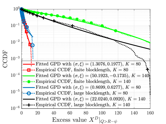
Figure 2: CCDF of the exceedance value fitted to GPD for various VUEs densities $K$ with deterministic arrivals, finite blocklength case with $L=550$.

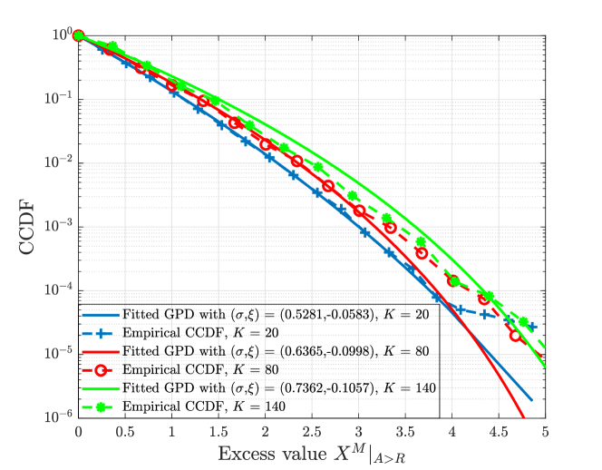
Figure 3: CCDF of the exceedance value fitted to GPD for various VUEs densities $K$ with Markovian arrivals, large blocklength case.

V-B Validation of Normal Approximation

In Fig. 4, we validate the accuracy of using normal approximation within our proposed framework. According to [32, Section IV-C], the normal approximation is quite accurate when transmitting at a large fraction of the channel capacity (e.g., 0.8 of channel capacity). Fig. 4 shows the CDF histogram of the rate to capacity ratio experienced within our simulations. Note that the transmission rate is equal to or larger than $0.8$ of the channel capacity about $99\%$ of the time, which verifies the accuracy of using normal approximation within our proposed framework.

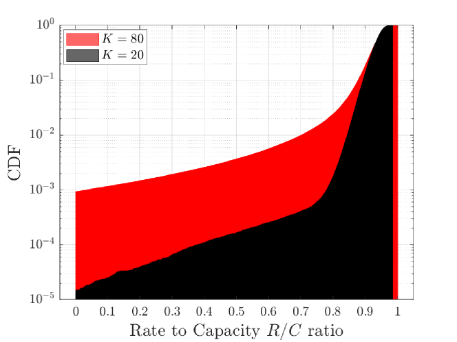
Figure 4: Histogram of the experienced rate to capacity ratio, for various densities of VUEs $K$ with deterministic arrivals, finite blocklength case.

V-C Performance Comparison Based on AoI

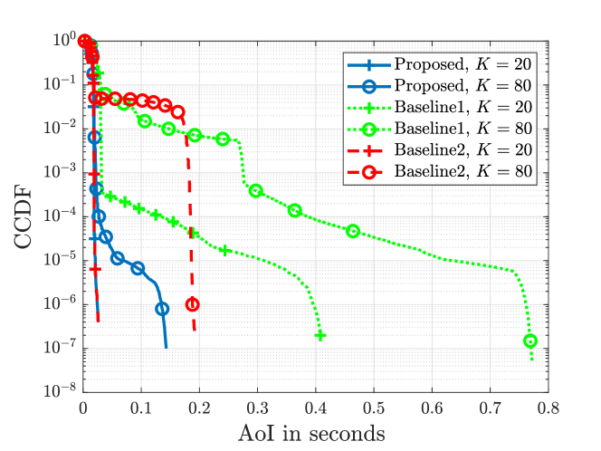
Figure 5: CCDF of the AoI for various densities of VUEs $K$ with deterministic arrivals, for large blocklength.

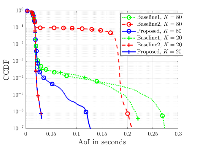
Figure 6: CCDF of the AoI for various densities of VUEs $K$ with deterministic arrivals, for finite blocklength with $L=550$.

In Fig. 5 and 6, the CCDFs of the AoI are plotted for the deterministic arrivals with large and finite blocklengths, with a comparison to Baseline 1 and Baseline 2. Note that, by using (4) the AoI can be calculated at the beginning of every time slot and then used to plot the CCDF. In particular, Fig. 5 and 6 show the AoI distributions for two densities of VUEs with large blocklength and finite blocklength ($L=550$ channel uses (CU)), respectively. From these two figures, we can see that the AoI performance for the proposed method outperforms the baseline models for both VUE densities, yielding improved reliability, except for Baseline 2 when $K=20$. For $K=20$, due to the low VUE density, each transmitter-receiver pair maintains high data rate yielding low-to-no events where AoI exceeding the threshold. Therefore, the constraints modeled using EVT to control the extreme events have no impact in which the proposed and Baseline 2 exhibit similar AoI distributions. Note that, as VUE density increases to $K=80$, increased interference and lower rates results in events with AoI exceeding the threshold. Therein, the proposed EVT-based constraints actively contribute to maintain the extreme AoI events whereas Baseline 2 has no control on such extreme events. As a result, the proposed method yields reduced AoI over the network compared to Baseline 2. From Fig. 5, we observe that, when $K=80$, Baseline 1 experiences at least $0.6\,s$ in AoI with $10^{-5}$ probability, while the proposed model experiences less than $0.1\,s$ for the same probability. Also, the probability of having the AoI greater than $0.1\text{ s}$ is more than $10^{-2}$ in the case of Baseline 2, while it is less than $10^{-5}$ in the proposed approach. In short, our proposed approach succeed in managing the AoI tail compared to the baselines.

V-D Impact of the Lyapunov Tradeoff Parameter $V$

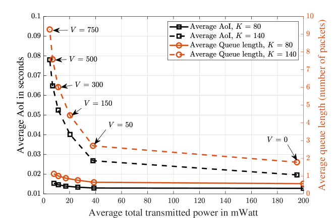
Figure 7: Transmit power, average AoI, and queue length trade-off for various VUEs densities $K$ with Markovian arrivals for large blocklength.

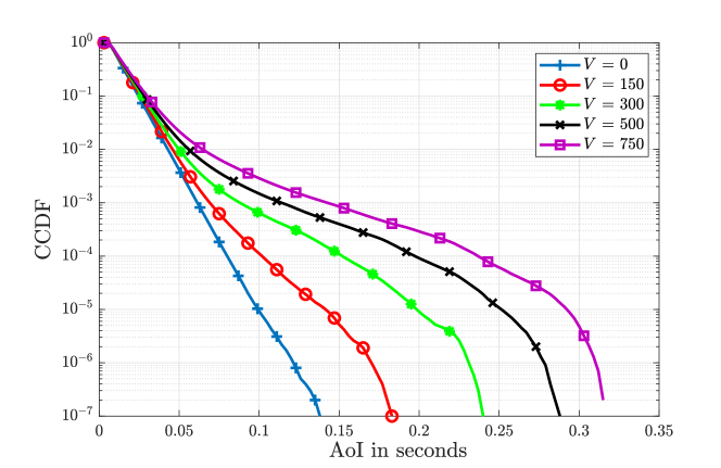
Figure 8: The AoI’s CCDF for various Lyapunov parameter $V$ when $K=80$ with Markovian arrivals for large blocklength.

Next, we discuss the impact of Lyapunov control parameter $V$ on the AoI and the optimal transmit power. In Luapunov optimization, $V$ controls the tradeoff between transmit power and queue stability. Therefore, the impacts of $V$ on AoI, queue length, and the transmission power on average are analyzed in Fig. 7 for two different VUE densities $K=\{80,140\}$ with the Markovian arrival case and large blocklength. It can be noted that, when $V$ is small, the priority of the VUEs is to minimize the physical and virtual queue lengths (i.e. maximize data rates) rather than minimizing the power consumption. Therefore, for small $V$, a smaller AoI can be observed at the price of an increased power consumption as illustrated in Fig. 7. In contrast, a large $V$ ensures a reduced power consumption with increased AoI. Fig. 7 shows that the average AoI and queue length of all VUE pairs in the Markovian arrival case increases as the Lyapunov parameter $V$ increases, while the total average transmitted power decreases.

Fig. 8 shows the CCDFs of AoI in the Markovian arrival case for different $V$. Similar to the average AoI, Fig. 8 validates our claim on the performance loss of overall AoI with increasing $V$. Although similar behavior can be observed for the deterministic arrival case, the differences are insignificant, in which the results are not presented.

V-E Impact of the Arrival Rate

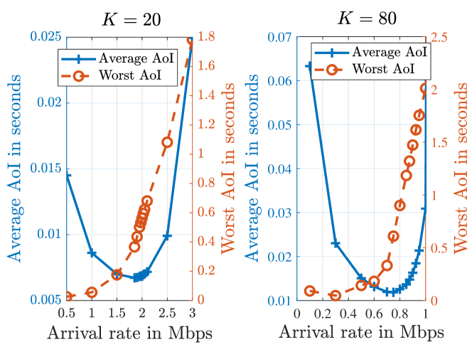
Figure 9: Arrival rate versus AoI trade-off, with $K=80$ and $K=20$ VUEs in the deterministic arrival case with large blocklength.

This subsection studies the impact of the status updates’ arrival rate for two different VUE densities, $K=80$ and $K=20$, for both average and worst AoI. The worst AoI is defined as the maximum AoI experienced by all VUEs during the simulation duration. Fig. 9 shows that, when the arrival rate is less than $0.1\text{ Mbps}$ ($0.5\text{ Mbps}$) when $K=80$ ($20$), the network experiences a higher average AoI. It also shows that increasing the arrival rate will lead to a better average AoI, up to a certain point (around $0.8\text{ Mbps}$ when $K=80$ and $2\text{ Mbps}$ when $K=20$), after which the average AoI starts increasing again. This happens because, at low arrival rates, queue stability is easily achieved. Thus, there is no rush of emptying the queue at the transmitter and data packets are more probable to be queued for a longer period, leading to a higher average AoI. When arrival rate increases, data packets within the queue are transmitted more frequently to maintain the queue stability. Thus, achieving lower average AoI. Further increasing the arrival rate will make it difficult to stabilize the queues. Hence, packets are lingered in the queue for longer duration, leading to the increased average AoI. Note that, at low VUE density ($K=20$), the network can withstand higher arrival rates. Fig. 9 also highlights that the worst AoI increases slightly with the arrival rate up to the aforementioned optimal arrival rate for the average AoI, and exhibits a rapid increase afterwards. Moreover, we note that the worst AoI is about 10 fold higher than the average AoI. Although the AoI achieves a small average, the worst AoI is heavy-tailed. In this situation, relying on the average AoI is inadequate for ensuring URLLC. This discrepancy between these two metrics demonstrates that the tail characterization is instrumental in designing and optimizing URLLC-enabled V2V networks.

V-F Impact of Blocklength $L$ and Block Error Probability $\varepsilon$

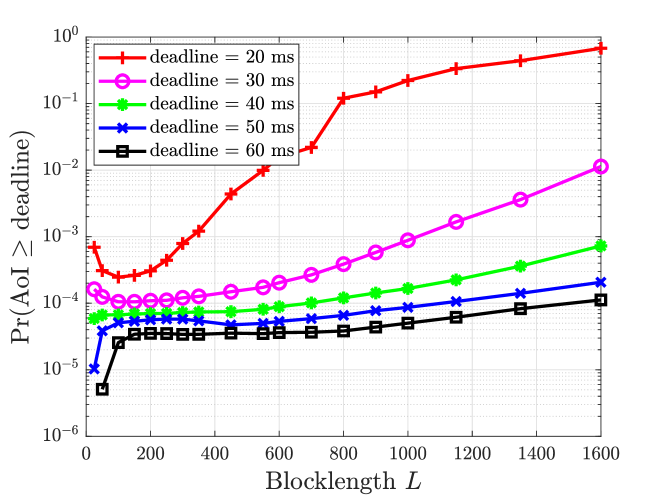
Figure 10: Blocklength $L$ vs. AoI violation probability, $K=80$ VUEs in the deterministic arrival case.

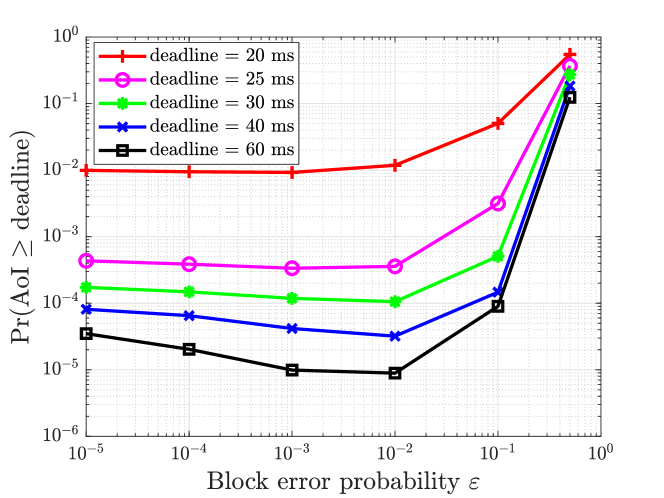
Figure 11: AoI violation probability vs. block error probability $\varepsilon$, $K=80$ VUEs in the deterministic arrival case.

Fig. 10 illustrates the effect of changing the blocklength $L$ on the probability of AoI exceeding a set of deadlines, $\textrm{Pr}\left\{\text{AoI}\geq\text{deadline}\right\}$. For a given $L$, e.g., when $L=550$, $\textrm{Pr}\left\{\text{AoI}\geq\text{deadline}\right\}$ can be computed from Fig. 6, where $\textrm{Pr}\left\{\text{AoI}\geq\text{deadline}\right\}$ is the actual achieved probability. Since the blocklength $L$ is determined by the bandwidth $\omega$ and the time slot duration (coherence time) $\tau$ as per $L=\omega\tau$, $L$ is varied by changing the coherence time $\tau$ (i.e., vehicle speed [44]). Fig. 10 shows that there exists a blocklength $L$ above which the AoI violation probability increases with increasing the blocklength $L$. Within this region, when the blocklength $L$ increases, both the transmission rate and transmit power consumption increase yielding more interference and, hence, the increase in the AoI violation probability. However, within the region where the blocklength and deadline are small, the small blocklength $L$ results in a small transmission rate and, hence, the packets are accumulated within the queue yielding a higher AoI violation probabilities. Moreover, for a fixed blocklength $L$, the AoI violation probability decreases with increasing the deadline. Finally, we show the impact of changing the block error probability $\varepsilon$ on the AoI violation probability in Fig. 11. Note that lowering the block error probability $\varepsilon$ decreases the transmission rate $R$ but increases the AoI. When $\varepsilon$ is large, e.g., $\varepsilon\in[10^{-2},0.5]$, the AoI violation probability is mainly caused by unsuccessful packet decoding. Thus, lowering $\varepsilon$ decrease the AoI violation probability. When $\varepsilon$ is below $10^{-3}$, the effect of unsuccessful packet decoding is not significant. In this regime, AoI violation is caused by the low transmission rate which results in a high AoI. Due to this reason, lowering $\varepsilon$ increases the AoI violation probability.

VI Conclusion and future work

In this paper, we have studied the problem of ultra-reliable and low-latency vehicular communication, considering both deterministic and stochastic arrivals . For this purpose, we have first defined a new reliability measure, in terms of probabilistic AoI, and have established a novel relationship between the AoI and queue-related probability distributions. Then, we have shown that characterizing the AoI tail distribution can be effectively done using EVT. Subsequently, we have formulated a transmit power minimization problem subject to the probabilistic AoI constraints and solved it using Lyapunov optimization. Furthermore, we have studied the impact of short packets and how it affects the optimization of AoI. Simulation results have shown that the proposed approach yields significant improvements in terms of AoI and queue length, when compared to baseline models. Moreover, an interesting tradeoff between the status updates’ arrival rate and the average and worst AoI achieved by the network has been exposed. We have also shown the existence of a blocklength at which the AoI violation probability is minimized. Many future extensions can be considered as follows: packet retransmissions, dynamic vehicle association, vehicles’ handover between RSUs, considering a multicast/broadcast scheme and finally, incorporating different queuing models and policies.

Appendix A Proof of Lemma 1

Since $T=\tau(t+1)$, then $\mathrm{Pr}\left\{T_{k}^{\text{D}}(\hat{\imath})>\tau(t+1)\right\}=\mathrm{Pr}\left\{\hat{\imath}\text{ is NOT served before time }\tau(t+1)\right\}$, which means that $\hat{\imath}$ is not served at or before time slot $t$. Subsequently, we apply (6) and derive

$$\mathrm{Pr}\left\{T_{k}^{\text{D}}(\hat{\imath})>\tau(t+1)\right\}$$

$$\overset{(a)}{=}\mathrm{Pr}\left\{\hat{\imath}>tA-1-\max\left(Q_{k}(t)-R_{k}(t),0\right)\right\}$$

$$\leq\mathrm{Pr}\left\{\frac{A}{\tau}(\tau(t+1)-d_{\text{D}})+1>tA-1-\left(Q_{k}(t)-R_{k}(t)\right)\right\}$$

$$=\mathrm{Pr}\left\{Q_{k}(t)>R_{k}(t)-\psi\right\},$$

where $\hat{\imath}=\lceil\frac{A}{\tau}(T-d_{\text{D}})\rceil\leq\frac{A}{\tau}(\tau(t+1)-d_{\text{D}})+1$ is used in step (a). It also should be noted that if $\hat{\imath}$ departs after $\tau(t+1)$, then $Q_{k}(t)-R_{k}(t)>0$, which is used in the same step.

Appendix B Proof of Lemma 2

Let $\check{\imath}$ be the last packet that departed at or just before time $T$. Thus, $\Delta_{k}(T)=T-T_{k}^{\text{A}}(\check{\imath})$.

Case 1: If no arrivals occurred during the time interval $\left[T-d_{\text{M}},T\right)$, then the arrival time of $\check{\imath}$ must be strictly less than $T-d_{\text{M}}$, i.e., $T_{k}^{\text{A}}\left(\check{\imath}\right)<T-d_{\text{M}}$. Therefore,

$$\mathrm{Pr}\left\{\Delta_{k}(T)>d_{\text{M}}\right\}=\mathrm{Pr}\left\{T-T_{k}^{\text{A}}\left(\check{\imath}\right)>d_{\text{M}}\right\}=1.$$

Case 2: If at least one arrival occurred during the time interval $\left[T-d_{\text{M}},T\right)$, then $T_{k}^{\text{A}}\left(\hat{\imath}\right)$ is bounded between $T-d_{\text{M}}\leq T_{k}^{\text{A}}\left(\hat{\imath}\right)<T$. Since $\hat{\imath}$ is the first arrival on or after time $T-d_{\text{M}}$, in this case, we need to show that the event $\left\{\Delta_{k}(T)<d_{\text{M}}\right\}$ is equivalent to the event $\left\{T_{k}^{\text{D}}(\hat{\imath})<T\right\}$ as in [14]. If the event $\left\{\Delta_{k}(T)<d_{\text{M}}\right\}$ occurred, then $T_{k}^{\text{A}}\left(\check{\imath}\right)\geq T-d_{\text{M}}$. By definition of $\hat{\imath}$, we should have $T_{k}^{\text{A}}\left(\hat{\imath}\right)\leq T_{k}^{\text{A}}\left(\check{\imath}\right)$ which entails that $T_{k}^{\text{D}}\left(\hat{\imath}\right)\leq T_{k}^{\text{D}}\left(\check{\imath}\right)\leq T$, due to FCFS assumption. As a result, $\left\{\Delta_{k}(T)<d_{\text{M}}\right\}\subseteq\left\{T_{k}^{\text{D}}(\hat{\imath})<T\right\}$.

To show equivalence of the two events, we show that the previous relation also holds the other way round. If event $\left\{T_{k}^{\text{D}}(\hat{\imath})<T\right\}$ occurred, we must have $T_{k}^{\text{A}}\left(\hat{\imath}\right)\leq T_{k}^{\text{A}}\left(\check{\imath}\right)$. Otherwise, $T_{k}^{\text{D}}(\check{\imath})<T_{k}^{\text{D}}(\hat{\imath})\leq T$ which contradicts the definition of $\check{\imath}$. Therefore, $\Delta_{k}(T)=T-T_{k}^{\text{A}}\left(\check{\imath}\right)\leq T-T_{k}^{\text{A}}\left(\hat{\imath}\right)\leq T-(T-d_{\text{M}})=d_{\text{M}}$. This implies that $\left\{T_{k}^{\text{D}}(\hat{\imath})<T\right\}\subseteq\left\{\Delta_{k}(T)<d_{\text{M}}\right\}$ and therefore, $\left\{\Delta_{k}(T)<d_{\text{M}}\right\}\equiv\left\{T_{k}^{\text{D}}(\hat{\imath})<T\right\}$.

Note that, due to the Poisson arrivals assumption. Using (14), the probability of no arrivals occurring during the time interval $\left[T-d_{\text{M}},T\right)$ (Case 1) is $e^{-\frac{\lambda d_{\text{M}}}{\tau}}$, while the probability of at least one arrival during the same interval (Case 2) is $1-e^{-\frac{\lambda d_{\text{M}}}{\tau}}$. Therefore, $\mathrm{Pr}\left\{\Delta_{k}(T)>d_{\text{M}}\right\}=1\cdot e^{-\frac{\lambda d_{\text{M}}}{\tau}}+\mathrm{Pr}\left\{T_{k}^{\text{D}}(\hat{\imath})>T\right\}\left(1-e^{-\frac{\lambda d_{\text{M}}}{\tau}}\right)$.

Appendix C Proof of Lemma 3

Since $\hat{\imath}$ is the packet that first arrives on or after time $T-d_{\text{M}}$, then $\mathrm{Pr}\left\{T_{k}^{\text{D}}(\hat{\imath})>T\right\}=\mathrm{Pr}\left\{\text{Sojourn time}>d_{\text{M}}\right\}$, where the sojourn time is the total time a packet spend within the system.

Observing the time slot $t$ and given that $R_{k}(t)$ is the number of packets that will be served during this slot, i.e. during period $\left[\tau t,\tau(t+1)\right]$. Therefore, $\left\{\text{Sojourn time}>d_{\text{M}}\right\}$ if the number of packets arrived during time period $\left[\tau t-d_{\text{M}},\tau(t+1)-d_{\text{M}}\right]$ is more than $R_{k}(t)$.

From (14), the Poisson distribution is irrelevant to the start and end times of a given period, therefore, $\mathrm{Pr}\biggl{\{}\text{Number of packets arrived during time period }\Bigl{[}\tau t-d_{\text{M}},\tau(t+1)-d_{\text{M}}\Bigr{]}>R_{k}(t)\biggr{\}}=\mathrm{Pr}\left\{A_{k}(t)>R_{k}(t)\right\}=\mathrm{Pr}\left\{\text{Sojourn time}>d_{\text{M}}\right\}$.

References

- [1] M. K. Abdel-Aziz, C.-F. Liu, S. Samarakoon, M. Bennis, and W. Saad, “Ultra-Reliable Low-Latency vehicular networks: Taming the age of information tail,” in Proc. of IEEE Global Commun. Conf., Dec. 2018.
- [2] G. Araniti, C. Campolo, M. Condoluci, A. Iera, and A. Molinaro, “LTE for vehicular networking: A survey,” IEEE Commun. Mag., vol. 51, no. 5, pp. 148–157, May 2013.
- [3] W. Saad, M. Bennis, and M. Chen, “A vision of 6g wireless systems: Applications, trends, technologies, and open research problems,” CoRR, vol. abs/1902.10265, 2019. [Online]. Available: http://arxiv.org/abs/1902.10265
- [4] T. Zeng, O. Semiari, W. Saad, and M. Bennis, “Joint communication and control for wireless autonomous vehicular platoon systems,” CoRR, vol. abs/1804.05290, 2018.
- [5] ETSI EN Std 302 637-2, “Intelligent transport systems; vehicular communications; basic set of applications; part 2: Specification of cooperative awareness basic service,” Aug. 2013.
- [6] M. Bennis, M. Debbah, and H. V. Poor, “Ultra-reliable and low-latency wireless communication: Tail, risk and scale,” Proc. IEEE, 2018, to be published.
- [7] S. Coles, An Introduction to Statistical Modeling of Extreme Values. Springer, 2001.
- [8] M. I. Ashraf, M. Bennis, C. Perfecto, and W. Saad, “Dynamic proximity-aware resource allocation in vehicle-to-vehicle (V2V) communications,” in Proc. IEEE Global Commun. Conf. Workshops, Dec. 2016, pp. 1–6.
- [9] M. I. Ashraf, C.-F. Liu, M. Bennis, and W. Saad, “Towards low-latency and ultra-reliable vehicle-to-vehicle communication,” in Proc. Eur. Conf. Netw. Commun., Jun. 2017, pp. 1–5.
- [10] T. Liu, Y. Zhu, R. Jiang, and Q. Zhao, “Distributed social welfare maximization in urban vehicular participatory sensing systems,” IEEE Trans. Mobile Comput., vol. 17, no. 6, pp. 1314–1325, Jun. 2018.
- [11] J. Mei, K. Zheng, L. Zhao, Y. Teng, and X. Wang, “A latency and reliability guaranteed resource allocation scheme for LTE V2V communication systems,” IEEE Trans. Wireless Commun., vol. 17, no. 6, pp. 3850–3860, Jun. 2018.
- [12] A. Mouradian, “Extreme value theory for the study of probabilistic worst case delays in wireless networks,” Ad Hoc Networks, vol. 48, pp. 1–15, Sep. 2016.
- [13] C.-F. Liu and M. Bennis, “Ultra-reliable and low-latency vehicular transmission: An extreme value theory approach,” IEEE Commun. Lett., vol. 22, no. 6, pp. 1292–1295, Jun. 2018.
- [14] J. Champati, H. Al-Zubaidy, and J. Gross, “Statistical guarantee optimization for age of information for the D/G/1 queue,” in Proc. IEEE Conf. Comput. Commun. Workshops, Apr. 2018.
- [15] ——, “Statistical guarantee optimization for AoI in single-hop and two-hop systems with periodic arrivals,” CoRR, vol. abs/1910.09949, 2019. [Online]. Available: http://arxiv.org/abs/1910.09949
- [16] S. Kaul, M. Gruteser, V. Rai, and J. Kenney, “Minimizing age of information in vehicular networks,” in Proc. IEEE Commun. Soc. Conf. on Sensor, Mesh and Ad Hoc Commun. and Netw., Jun. 2011, pp. 350–358.
- [17] A. Kosta, N. Pappas, and V. Angelakis, “Age of information: A new concept, metric, and tool,” Foundations and Trends in Networking, vol. 12, no. 3, pp. 162–259, 2017.
- [18] Y. Sun, T. Z. Ornee, and M. K. C. Shisher, “The ongoing history of the age of information,” 2019. [Online]. Available: http://webhome.auburn.edu/ yzs0078/AoI.html
- [19] Z. Chen, N. Pappas, E. Björnson, and E. G. Larsson, “Optimal control of status updates in a multiple access channel with stability constraints,” CoRR, vol. abs/1910.05144, 2019. [Online]. Available: http://arxiv.org/abs/1910.05144
- [20] B. T. Bacinoglu, Y. Sun, E. Uysal, and V. Mutlu, “Optimal status updating with a finite-battery energy harvesting source,” CoRR, vol. abs/1905.06679, 2019. [Online]. Available: http://arxiv.org/abs/1905.06679
- [21] A. Baiocchi and I. Turcanu, “A model for the optimization of beacon message age-of-information in a VANET,” in Proc. IEEE 29th Int. Teletraffic Congress, vol. 1, Sep. 2017, pp. 108–116.
- [22] M. A. Abd-Elmagid and H. S. Dhillon, “Average age-of-information minimization in UAV-assisted IoT networks,” CoRR, vol. abs/1804.06543, 2018.
- [23] Y. Inoue, H. Masuyama, T. Takine, and T. Tanaka, “A general formula for the stationary distribution of the age of information and its application to single-server queues,” CoRR, vol. abs/1804.06139, 2018.
- [24] R. Devassy, G. Durisi, G. C. Ferrante, O. Simeone, and E. Uysal-Biyikoglu, “Delay and peak-age violation probability in short-packet transmissions,” in Proc. IEEE Int. Symp. Inf. Theory, Jun. 2018.
- [25] M. Costa, M. Codreanu, and A. Ephremides, “On the age of information in status update systems with packet management,” IEEE Trans. Inf. Theory, vol. 62, no. 4, pp. 1897–1910, Apr. 2016.
- [26] L. Huang and E. Modiano, “Optimizing age-of-information in a multi-class queueing system,” in Proc. IEEE Int. Symp. Inf. Theory, Jun. 2015, pp. 1681–1685.
- [27] Q. He, D. Yuan, and A. Ephremides, “On optimal link scheduling with min-max peak age of information in wireless systems,” in IEEE Int. Conf. Commun., May 2016, pp. 1–7.
- [28] M. J. Neely, Stochastic Network Optimization with Application to Communication and Queueing Systems. Morgan and Claypool Publishers, Jun. 2010.
- [29] F. F. Hassanzadeh and S. Valaee, “Reliable broadcast of safety messages in vehicular ad hoc networks,” in Proc. IEEE Conf. Comput. Commun., Apr. 2009, pp. 226–234.
- [30] M. Wang, M. Winbjork, Z. Zhang, R. Blasco, H. Do, S. Sorrentino, M. Belleschi, and Y. Zang, “Comparison of LTE and DSRC-based connectivity for intelligent transportation systems,” in Proc. IEEE 85th Veh. Technol. Conf. (VTC-Spring), Jun. 2017, pp. 1–5.
- [31] G. Durisi, T. Koch, and P. Popovski, “Toward massive, ultrareliable, and low-latency wireless communication with short packets,” Proc. IEEE, vol. 104, no. 9, pp. 1711–1726, Sep. 2016.
- [32] Y. Polyanskiy, H. V. Poor, and S. Verdu, “Channel coding rate in the finite blocklength regime,” IEEE Trans. Inf. Theory, vol. 56, no. 5, pp. 2307–2359, May 2010.
- [33] F. Bai, N. Sadagopan, and A. Helmy, “IMPORTANT: A framework to systematically analyze the impact of mobility on performance of routing protocols for adhoc networks,” in Proc. IEEE Conf. Comput. Commun., vol. 2, Mar. 2003, pp. 825–835.
- [34] ETSI, “Ts 102 940: Intelligent transport systems (its),” Security, ITS communications security architecture and security management, pp. 2012–03.
- [35] ——, “Tr 102 638 v1,” 0.7, Technical Report, Intelligent Transport Systems (ITS), Tech. Rep.
- [36] M. Abdulla and H. Wymeersch, “Fine-grained vs. average reliability for V2V communications around intersections,” in Proc. IEEE Global Commun. Conf. Workshops, Dec. 2017, pp. 1–5.
- [37] C. Liu, M. Bennis, M. Debbah, and H. V. Poor, “Dynamic task offloading and resource allocation for ultra-reliable low-latency edge computing,” IEEE Trans. Commun., pp. 1–1, 2019.
- [38] C.-F. Liu, M. Bennis, and H. V. Poor, “Latency and reliability-aware task offloading and resource allocation for mobile edge computing,” in Proc. IEEE Global Commun. Conf. Workshops, Dec. 2017, pp. 1–7.
- [39] U. von Luxburg, “A tutorial on spectral clustering,” Statistics and Computing, vol. 17, no. 4, pp. 395–416, Dec. 2007.
- [40] S. Tsironis, M. Sozio, M. Vazirgiannis, and L. Poltechnique, “Accurate spectral clustering for community detection in mapreduce,” in Proc. Adv. in Neural Inf. Process. Syst. (NIPS) Workshops. Citeseer, 2013.
- [41] A. Lancho, J. Östman, G. Durisi, T. Koch, and G. Vazquez-Vilar, “Saddlepoint approximations for rayleigh block-fading channels,” CoRR, vol. abs/1904.10442, 2019. [Online]. Available: http://arxiv.org/abs/1904.10442
- [42] M. Shirvanimoghaddam, M. S. Mohammadi, R. Abbas, A. Minja, C. Yue, B. Matuz, G. Han, Z. Lin, W. Liu, Y. Li, S. Johnson, and B. Vucetic, “Short block-length codes for ultra-reliable low latency communications,” IEEE Communications Magazine, vol. 57, no. 2, pp. 130–137, February 2019.
- [43] T. Lipp and S. Boyd, “Variations and extension of the convex–concave procedure,” Optim. Eng., vol. 17, no. 2, pp. 263–287, Jun. 2016.
- [44] Z. Pi and F. Khan, “System design and network architecture for a millimeter-wave mobile broadband (MMB) system,” in Proc. IEEE 34th Sarnoff Symp., May 2011, pp. 1–6.