Genealogies and inference for populations with highly skewed offspring distributions

Abstract.

We review recent progress in the understanding of the role of multiple- and simultaneous multiple merger coalescents as models for the genealogy in idealised and real populations with exceptional reproductive behaviour. In particular, we discuss models with ‘skewed offspring distribution’ (or under other non-classical evolutionary forces) which lead in the single locus haploid case to multiple merger coalescents, and in the multi-locus diploid case to simultaneous multiple merger coalescents. Further, we discuss inference methods under the infinitely-many sites model which allow both model selection and estimation of model parameters under these coalescents.

1. Multiple merger coalescents in population genetics

1.1. Introduction

The ‘standard’ model in mathematical population genetics is Kingman’s coalescent [46], which describes on appropriate time scales the random genealogies of a large class of population models. A salient feature of models in the domain of attraction of Kingman’s coalescent and its ramifications is that, at least in the limit of large population size, only binary mergers of ancestral lineages are visible. This is owed to the fact that the number of offspring of any individual must be negligible in comparison with the total population size.

It is an important and very useful universality feature of Kingman’s coalescent that as the population size $N\to\infty$, the details of the actual offspring distribution are ‘washed out’ from the limit model, only its variance $\sigma_{N}^{2}\to\sigma^{2}\in(0,\infty)$ remains as a time-rescaling compared to the ‘standard’ Kingman coalescent. A crucial assumption here is $\sigma^{2}<\infty$.

The question ‘what if $\sigma^{2}=\infty$?’ is also biologically relevant: While all real populations are finite, coalescent theory is about (tractable) limit results as $N\to\infty$, and $\sigma^{2}=\infty$ really means that $\sigma^{2}_{N}$ is large when $N$ is large. As we will see below, there is a variety of biological mechanisms which predict a deviation from the Kingman coalescent model.

In this article, we will first describe general coalescent models (where the term ‘general’ means that multiple- and even simultaneous multiple mergers of ancestral lineages will be allowed), and review briefly population models that lead to limiting genealogies described by certain subclasses of these general coalescent processes. We will then investigate how one of the most popular statistics of real DNA sequence data (under the infinitely many sites model), namely the site-frequency spectrum, behaves under these coalescent models, and then derive inference methods that allow to estimate evolutionary parameters within a certain class of coalescent models, or to distinguish between different underlying genealogical models. While this theory is mostly confined to single-locus data of haploid populations, we will finally derive the genealogy in a simple diploid multi-locus model. Interestingly, this will naturally lead to genealogies driven by coalescents with simultaneous multiple mergers. Also, the additional information contained in multi-locus data will, despite dependence between different loci that is inherent in multiple-merger coalescent even in the face of high recombination rates, increase the statistical power of our methods for inference.

We conclude this text with an outlook on recent developments in the field and the potential relevance of our results. To sum up, we aim to take steps towards understanding in how far the conjecture of Eldon & Wakeley ([28], p. 2622) holds:

‘It may be that Kingman’s coalescent applies only to a small fraction of species. For many species, the coalescent with multiple mergers might be a better null model than Kingman’s coalescent.’

Note that this article is related to several others in this volume that also touch upon the topic of non-standard genealogies, in particular those by Fabian Freund, by Götz Kersting and Anton Wakolbinger and by Anja Sturm. We will highlight concrete links in the sequel.

1.2. Multiple and simultaneous multiple merger coalescents

About two decades ago, two natural classes of general coalescent processes, the so-called $\Lambda$-coalescents [52, 56, 23] and $\Xi$-coalescents [59, 50] were introduced in the mathematical literature. All these coalescents have in common that they are (exchangeable) partition-valued continuous-time Markov chains, that is, they take values in the space $\mathcal{P}_{n}$, the space of finite partition of $[n]:=\{1,\ldots,n\}$ if started from a finite number of blocks. Both of the above classes of coalescent processes allow multiple mergers of ancestral lines, by which we mean a transition that is obtained from the current partition state by merging a certain number of blocks (representing ancestral lines) into one or several new blocks, thus obtaining a ‘coarser partition’. In the case of the classical Kingman coalescent, these transitions are always binary, that is, precisely two blocks merge into one new block.

In the case of a $\Lambda$-coalescent, however, at transition times, multiple lines necessarily merge into one single new block, while for $\Xi$-coalescents, subsets of blocks involved in a coalescence event may merge into different ‘target blocks’.

The path of an $n$-coalescent process corresponds in a natural way to a random tree where the leaves correspond to $\{1\},\{2\},\dots,\{n\}$ and internal nodes to larger blocks. In fact, one can interpret a coalescent as a random metric space; see e.g. [32] and [37, 38].

In this article, we only consider coalescent processes starting from finitely many blocks (i.e., $n$-coalescents). The corresponding coalescents with $n=\infty$ can be constructed by employing consistency and using Kolmogorov’s extension theorem, or explicitly via look-down constructions [23, 13]. They have very interesting mathematical properties which are, however, not in the focus of this text. Let us first briefly introduce the pertinent notation.

1.2.1. Multiple merger (MMC) coalescents

For $\pi\in\mathcal{P}_{n}$ let $|\pi|$ denote the number of blocks and for $\pi,\pi^{\prime}\in\mathcal{P}_{n}$ we write $\pi^{\prime}\prec_{m,k}\pi$ if $|\pi|=m$ and $\pi^{\prime}$ arises from $\pi$ by merging $k$ blocks into a single one (a ‘$k$-merger’).

For a finite measure $\Lambda$ on $[0,1]$, define

(1.1) $$\lambda_{m,k}:=\int_{0}^{1}x^{k-2}(1-x)^{m-k}\Lambda(dx),\quad\lambda_{m}:=\sum_{k=2}^{m}\binom{m}{k}\int_{0}^{1}x^{k-2}(1-x)^{m-k}\Lambda(dx).$$

The $n$-$\Lambda$-coalescent is a $\mathcal{P}_{n}$-valued continuous-time Markov chain $\{\Pi_{t}^{(\Lambda)},t\geqslant 0\}$ with transition rates $q_{\pi,\pi^{\prime}}$ from $\pi$ to $\pi^{\prime}\neq\pi$ given by

(1.2) $$q_{\pi,\pi^{\prime}}=\begin{cases}\lambda_{m,k}&\textrm{if $\pi^{\prime}\prec_{m,k}\pi$ for some $k$,}\\ 0&\textrm{otherwise.}\\ \end{cases}$$

Remark 1.1.

A natural interpretation of (1.1) is to imagine that for $x\in(0,1]$ at rate $x^{-2}\Lambda(dx)$, a ‘merging event of size $x$’ occurs: In such an event, every block independently flips a ‘coin’ with success probability $x$ and all the ‘successful’ blocks are merged. In fact, such constructions are in [52, 23] and this intuition is also corroborated by the duality with the $\Lambda$-Fleming-Viot process (see page 1.3).

Obviously, the class of all $\Lambda$-coalescents (corresponding to all the finite measures on $[0,1]$) is quite large and in particular non-parametric. The following important special cases have frequently appeared in the literature:

Example 1.2.

• The Kingman coalescent $\Pi^{\tt(K)}$ [46] corresponds to the choice

  $$\Lambda(dx)=\delta_{0}(dx).$$

  i.e. $\Pi^{\tt(K)}=\Pi^{(\delta_{0})}$. Here, the measure $\Lambda$ is concentrated on the point $0$ and no multiple, only binary mergers happen, as is evident from (1.1).

• The ‘star-shaped coalescent’ coalescent $\Pi^{\tt(S)}$ corresponds to the choice

  $$\Lambda(dx)=\delta_{1}(dx).$$

  This coalescent exhibits only one single transition, in which all active lines merge into a single line within one step.

• The Bolthausen-Sznitman coalescent $\Pi^{\tt(BS)}$, introduced in [16] as a tool to study certain spin glass models in statistical mechanics, is given by

  $$\Lambda(dx)={\bf 1}_{[0,1]}(x)(dx),$$

  i.e. when the measure $\Lambda$ is the uniform distribution on $[0,1]$.

• The Beta$(2-\alpha,\alpha)$-coalescent $\Pi^{\tt(B)}$ is given by

  $$\Lambda(dx)=\frac{\Gamma(2)}{\Gamma(2-\alpha)\Gamma(\alpha)}x^{1-\alpha}(1-x)^{\alpha-1}\,dx,$$

  with $\alpha\in(0,2)$. Here, the measure $\Lambda$ is associated with the beta distribution with parameters $2-\alpha$ and $\alpha$. The limiting case $\alpha=2$ (in the sense of weak convergence of measures) corresponds to the Kingman coalescent, while $\alpha=1$ returns the Bolthausen-Sznitman-coalescent $\Pi^{\tt(BS)}$ and (the weak limit) $\alpha\to 0$ gives the star-shaped coalescent $\Pi^{\tt(S)}$.

  For a visual impression of realisations of Beta-coalescent trees for different values of $\alpha$ we refer to the contribution by Götz Kersting and Anton Wakolbinger in this volume. in the article by G. Kersting and A. Wakolbinger in this volume.

• The following class of purely atomic coalescents has been investigated by [28]: Here, one considers the cases

  $$\Lambda(dx)=\delta_{\psi}(dx),$$

  and

  $$\Lambda(dx)=\frac{2}{2+\psi^{2}}\delta_{0}(dx)+\frac{\psi^{2}}{2+\psi^{2}}\delta_{\psi}(dx),$$

  with $\psi\in[0,1]$, where $\psi=0$ gives the Kingman coalescent.

We refer to [33] and [5] for surveys on $\Lambda$-coalescents. See also the contribution by G. Kersting and A. Wakolbinger in this volume.

1.2.2. Simultaneous multiple merger (SMMC) coalescents

Formulating the dynamics of a SMMC requires some notational overhead but we will see that they appear naturally as genealogies in diploid population models with highly skewed offspring distributions. For

(1.3) $$\underline{k}=(k_{1},k_{2},\dots,k_{r})\quad\text{with }r\in\mathbb{N},\;k_{1}\geqslant k_{2}\geqslant\cdots\geqslant k_{r}\geqslant 2$$

and $\pi,\pi^{\prime}\in\mathcal{P}_{n}$ with $|\pi|=m$ we write $\pi^{\prime}\prec_{m,\underline{k}}\pi$ if $\pi^{\prime}$ arises from $\pi$ by merging $r$ groups of blocks of sizes $k_{1},k_{2},\dots,k_{r}$ (and leaving the other blocks unchanged). We write $|\underline{k}|=k_{1}+\cdots+k_{r}$.

In order to describe the dynamics of a SMMC, we need a bit of notation: Let $\Delta$ denote the infinite simplex

$$\Delta:=\left\{\boldsymbol{x}=(x_{1},x_{2},\ldots):x_{1}\geqslant x_{2}\geqslant\cdots\geqslant 0,\quad\sum_{i}x_{i}\leqslant 1\right\}$$

and let $\Delta_{\boldsymbol{0}}:=\Delta\setminus\{(0,0,\ldots)\}=\Delta\setminus\{\boldsymbol{0}\}.$ Let $\Xi_{0}$ be a finite measure on $\Delta_{\boldsymbol{0}}$, $a>0$, then $\Xi:=a\delta_{\mathbf{0}}+\Xi_{0}$ is a finite measure on $\Delta$.

For $\underline{k}$ as in (1.3), with $s=m-|\underline{k}|$, put

$$\lambda_{m,\underline{k}} =a\boldsymbol{1}_{(r=1,k_{1}=2)}$$

(1.4) $$\quad+\int\limits_{\Delta_{\boldsymbol{0}}}\dfrac{\sum\limits_{\ell=0}^{s}\sum\limits_{i_{1}\neq\ldots\neq i_{r+\ell}}\binom{s}{\ell}x_{i_{1}}^{k_{1}}\cdots x_{i_{r}}^{k_{r}}x_{i_{r+1}}\cdots x_{i_{r+\ell}}\left(1-\sum_{j}x_{j}\right)^{s-\ell}}{\sum_{j}x_{j}^{2}}\,\Xi_{\boldsymbol{0}}(d\boldsymbol{x})$$

An $n$-$\Xi$-coalescent $\{\Pi^{\Xi}_{t}\}$ is a continuous-time Markov chain on $\mathcal{P}_{n}$ which jumps from $\pi\in\mathcal{P}_{n}$ with $|\pi|=m$ to $\pi^{\prime}\in\mathcal{P}_{n}$ at rate $q_{\pi,\pi^{\prime}}=\lambda_{m,\underline{k}}$ if $\pi^{\prime}\prec_{m,\underline{k}}$ with $\underline{k}$ as in (1.3), and $q_{\pi,\pi^{\prime}}=0$ if $\pi^{\prime}\neq\pi$ is not of this form.

The form of the jump rates (1.2.2) has a similar interpretation as discussed in Remark 1.1 for the case of $\Lambda$-coalescents: At rate $a$, pairwise merging occurs. Furthermore, for $\mathbf{x}=(x_{1},x_{2},\dots)\in\Delta_{\boldsymbol{0}}$, at rate $(\sum_{j}x_{j}^{2})^{-1}\Xi_{0}(dx)$ an ‘$x$-merging event’ occurs. In such an event, every block independently draws a ‘colour,’ where colour $i$ is drawn with probability $x_{i}$ for $i\geqslant 1$ and colour $0$ with probability $1-|\mathbf{x}|$. Then all blocks with the same colour $i$ for $i\geqslant 1$ are merged.

Obviously, the class of $\Xi$-coalescents is even richer than the class of $\Lambda$-coalescents. In particular, one recovers a $\Lambda$-coalescent by choosing $\Xi:=\Lambda\otimes\delta_{0}\otimes\delta_{0}\otimes\cdots,$ i.e. if $\Xi$ is concentrated on the first component of the simplex. However, only a handful of natural examples have been motivated and analysed on the basis of an underlying population model so far. The following important special cases have appeared in the literature:

Example 1.3.

• Let $PD_{\theta}$ be the Poisson-Dirichlet distribution with $\theta>0$. The Poisson-Dirichlet coalescent with $\Xi=\left(\sum_{i}x_{i}^{2}\right)^{-1}\!PD_{\theta}$ appears in [57] as the genealogy of the ‘Dirichlet compound Wright–Fisher model.’

• Subordinated Kingman-coalescents. If one applies a discontinuous time-change to a Kingman coalescent, as soon as more than one binary coalescence event of the original process falls into a jump-interval of the time-change, one obtains a multiple or simultaneous multiple merger event. When the (random) time-change is given by a subordinator $\{S_{t}\}$, the time-changed process $\{\Pi^{\tt(K)}_{S_{t}}\}_{t\geqslant 0}$ is a $\Xi$-coalescent. The representation of $\Xi$ in terms of $\{S_{t}\}$ as mixture of Dirichlet distributions is non-trivial and omitted here for brevity, see [13, Prop. 6.3] for a partial answer. See also [31] for the related class of ‘symmetric coalescents’.

• R. Durrett and J. Schweinsberg [26] approximate the genealogy in a selective sweep by a $\Xi$-coalescent, where $\Xi$ is described by a stick-breaking construction, see [26, Section 3].

• In diploid bi-parental populations, in which the reproduction events of each parent are governed by a certain $\Lambda$-coalescent, one obtains genealogies given by $\Xi-$coalescents of the form

  $$\Xi=\frac{1}{4}\int_{[0,1]}\delta_{(x/4,\,x/4,\,x/4,\,x/4,\,0,\,0,\,0,\,\dots)}\,\Lambda(dx)$$

  In particular, the cases $\Lambda=\delta_{\psi}$ and $\Lambda=\mathrm{Beta}(2-\alpha,\alpha)$ for suitable $\psi$ and $\alpha$ have been considered, see [11]. The reason for the fourfold split is that the ancestral line of a chromosome may merge into any of the four parental chromosome (two for each parent). Such $\Xi$-coalescents will play an important role in Section 3 below.

1.3. Population models

A substantial amount of work has been devoted to understanding conditions under which population models converge to limits whose genealogy can be described by one of the above coalescent processes. Typically, one considers populations of fixed size $N$, whose reproductive event can be described by exchangeable offspring distributions.

A full classification of offspring distributions and time scalings in Cannings-models for convergence to $\Lambda$- and $\Xi$-coalescents has been found in [50]. It is thus possible to provide abstract criteria and descriptions for population models that make their ancestral distributions converge to any prespecified $\Xi-$ or $\Lambda-$coalescent.

However, the relevance of a particular (SMMC) model clearly depends on its plausibility as limit of a in some sense natural population model. We thus now briefly review such population models and their genealogical coalescent limits.

• Beta$(2-\alpha,\alpha)$-coalescents with $\alpha\in(1,2]$ are obtained as limiting genealogy of Schweinsberg’s model [60], in which individuals produce in a first step potential offspring according to a stable law with index $\alpha$ and mean $m>1$, and then $N$ out of these are selected for survival. This corresponds to what is known as a ‘highly skewed offspring distribution’ or ‘sweepstakes reproduction’ (cf. [1, 40, 41]). In population biology, it resembles so-called ‘type-III survivorship’, that is, high fertility leading to excessive amounts of offspring, corresponding to the first reproduction step, whereas high mortality early in life is modelled in the second step. Several authors have proposed this class of coalescents to describe the reproductive behaviour of Atlantic cod (see e.g. [64, 2]).

  One can see heuristically why this particular form of the $\Lambda$-measure appears: The probability that a given individual’s offspring provides more than fraction $y$ of the next generation, given that the family is substantial (i.e. given $X_{1}\geqslant\varepsilon N$, for $y>\varepsilon$), is approximately

  $$\hskip 40.00006pt\mathbb{P}\hskip 0.5pt\Big{(} \frac{X_{1}}{X_{1}+(N-1)m}\geqslant y\mid X_{1}\geqslant\varepsilon N\Big{)}$$

  $$\hskip 40.00006pt=\mathbb{P}\hskip 0.5pt\Big{(}{X_{1}}\geqslant\frac{(N-1)my}{1-y}\mid X_{1}\geqslant\varepsilon N\Big{)}$$

  $$\hskip 40.00006pt\sim\,\text{const.}\times\frac{(1-y)^{\alpha}}{y^{\alpha}}=\text{const.}\times\mathrm{Beta}(2-\alpha,\alpha)([y,1]),$$

  where we replaced $X_{2}+\cdots+X_{n}\approx(N-1)m$ by the law of large numbers. The model is also mathematically appealing, since it exhibits a close connection to renormalised $\alpha$-stable branching processes, see [14].

• Huillet’s Pareto model: [44] derives $\mathrm{Beta}(2-\alpha,\alpha)$-coalescents as limiting genealogies in a population model similar to the one in (B) where the sampling can be interpreted as according to a ‘random fitness value.’

• The Bolthausen-Sznitman coalescent appears for $\alpha=1$ in the sweepstakes model, but also as limiting genealogy at the ‘tip of a fitness wave.’ This was predicted in [18] using non-rigorous arguments (for a related model also [51]), and partly confirmed (for certain variations of the model) in [7], [61, 62].

• This model corresponds to populations, in which in each reproductive step, a fraction of $\psi$ individuals are produced by one single parent. This can be combined with classical Wright-Fisher type reproduction to produce the ‘Kingman atom’ at 0. See [28].

• Generalised Moran models. Independently in each reproduction event, a random number $\Psi^{(N)}$ of offspring are born to a single pair of parents, these offspring replace $\Psi^{(N)}$ randomly chosen individuals from the present population. $\mathbb{P}\hskip 0.5pt(\Psi^{(N)}=1)=1$ corresponds to the classical Moran model; (EW) is also a special case of this. By suitably choosing $\mathcal{L}(\Psi^{(N)})$ one can in fact approximate any $\Lambda$-coalescent, see Section 3.1.

• Appear as scaling limits of diploid bi-parental models with skewed reproduction. We will present a corresponding model in Section 3.1. A complete classification of the corresponding diploid population limits can be found in [9].

See also Tellier and Lemaire [66] for a recent overview from a biological perspective. There are many further extensions of population and coalescent models in the literature, including spatial models such as Barton, Etheridge and Véber’s spatial $\Lambda$-Fleming Viot process [3], or so-called on/off coalescents in situations with seed banks, see, e.g., the contribution by the second author together with Noemi Kurt in this volume. However, in this article, our focus is the reproductive mechanism of neutral well-mixed populations, so that we refrain from providing a further discussion of these models here.

All of the above coalescent processes are dual to the corresponding forward-in-time population limit, given as a (generalised) Fleming-Viot process (which is a measure-valued (jump-)diffusion), [23] and e.g. [8].

Details of this and a representation of the generator of $\Xi$-coalescents can be found in [13]. There, it is also shown that the above duality can be strengthened to a strong pathwise duality via an extension of Donnelly and Kurtz’ celebrated lookdown-construction [22, 23].

2. Inference based on the site-frequency spectrum

One of the most important and well-studied statistical quantities derived from DNA sequence data is the site frequency spectrum (SFS). For the theoretical analysis, we assume that all underlying data fits to the infinitely-many-sites model (IMS) of population genetics (cf. [69] or [67]), that is, we assume that every observed site mutated at most once during the entire history of the sample. This assumption is often at least approximately true since typical per-site mutation rates are very small. Here, ‘site’ refers to a single base pair in the DNA molecule. Furthermore, from a pragmatical point of view, the SFS of a dataset is well-defined even if the assumptions of the IMS model are violated (see, e.g., [39] for the combinatorial characterisation of data complying with the IMS model).

For the analysis, we also assume that the genealogy of a sample of size $n\in\mathbb{N}$ is described by one of the above coalescent models $\Pi$ and that mutations occur at some rate $\theta/2>0$ on the coalescent branches, see Figure 2.1 for an illustration. If we know the ancestral state, then, the SFS of an $n$-sample is defined as

$${\boldsymbol{\xi}}^{(n)}:=\big{(}\xi_{1}^{(n)},\dots,\xi^{(n)}_{n-1}\big{)},$$

where $\xi^{(n)}_{i},i\in[n-1]$ is the number of sites at which a mutation appears $i$-times in our sample.

If the ancestral states are unknown (and thus the data matrix as in Figure 2.1 is only defined up to column-flips), one considers instead the folded site frequency spectrum ($\delta_{i,j}$ is the Kronecker delta)

$${\boldsymbol{\eta}}^{(n)}:=\Big{(}\eta_{1}^{(n)},\dots,\eta^{(n)}_{\lfloor n/2\rfloor}\Big{)}\quad\text{with }\eta^{(n)}_{i}=\xi^{(n)}_{i}+\big{(}1-\delta_{i,n-i}\big{)}\xi^{(n)}_{n-i},\quad i=1,\dots,\lfloor n/2\rfloor.$$

Mutations on a coalescent tree and resulting data matrix (in schematic form). Implicitly, identical columns are removed from the data matrix. The corresponding SFS is ${\boldsymbol{\xi}}^{(5)}=(4,2,1,0)$.

Figure 2.1.  

2.1. The expected site frequency spectrum

For a coalescent process $\Pi=\{\Pi_{t}\}_{t\geqslant 0}$ with mutation rate $\theta$ we denote its law by $\mathbb{P}\hskip 0.5pt^{\Pi,\theta}$, that is, the law of the coalescent process $\Pi$ on which mutations appear along its branches at rate $\theta/2$. We denote the expectation corresponding to $\mathbb{P}\hskip 0.5pt^{\Pi,\theta}$ by $\mathbb{E}^{\Pi,\theta}$. Recall that the block-counting process $Y=\{Y_{t}\}_{t\geqslant 0}$ of the coalescent process $\Pi$

(2.1) $$Y_{t}:=|\Pi_{t}|,\quad t\geqslant 0,$$

simply counts the number of ancestral lineages present at each time. Then, a general representation of $\mathbb{E}^{\Pi,\theta}\big{[}\xi_{i}^{(n)}\big{]}$ for any coalescent model $\Pi$ (see [36]) is

(2.2) $$\mathbb{E}^{\Pi,\theta}\left[\xi_{i}^{(n)}\right]=\frac{\theta}{2}\sum_{k=2}^{n-i+1}{p^{(n),\Pi}[k,i]}\cdot k\cdot\mathbb{E}^{\Pi}\left[T_{k}^{(n)}\right],\quad i\in[n-1],$$

where $T_{k}^{(n)}$ is the random amount of time that $\{Y_{t}\}_{t\geqslant 0}$, starting from $Y_{0}=n$, spends in state $k$, and $p^{(n),\Pi}[k,i]$ is the probability that conditional on the event that $Y_{t}=k$ for some time point $t$, a given one of these $k$ blocks subtends exactly $i\in[n-1]$ leaves. Thus, in (2.2) mutations are classified according to the ‘level’ $k$, which is the value of the block-counting process when they appear in the tree.

2.1.1. The block-counting process

For brevity, we consider only $\Lambda$-coalescents $\Pi$ in this paragraph. We see from (1.2) that $Y$ corresponding to $\Pi$ from (2.1) is itself a continuous-time Markov chain on $\mathbb{N}$ (as $\lambda_{\pi,\pi^{\prime}}$ depends only on $\pi$ and $\pi^{\prime}$) with jump rates

$$q_{ij}={i\choose i-j+1}\lambda_{i,i-j+1},\quad i>j\geqslant 1.$$

The total jump rate away from state $i$ is $-q_{ii}=\sum_{j=1}^{i-1}q_{ij}$.

We will need the Green function of $Y$,

(2.3) $$g(n,m):=\mathbb{E}_{n}\left[\int_{0}^{\infty}{\bf 1}_{(Y_{s}=m)}\,ds\right]\quad\mbox{for $\quad n\geqslant m\geqslant 2$}.$$

For the Kingman coalescent, we have $g(n,m)=\frac{2}{m(m-1)}$ for $m\leqslant n$, for the Bolthausen-Sznitman coalescent, explicit expressions can be obtained from [49]. In general, there is no explicit formula for (2.3), but decomposing according to the first jump of $Y$ gives a recursion for $g(n,m)$:

(2.4) $$g(n,m)=\sum_{k=m}^{n-1}p_{nk}g(k,m),\;\;n>m\geqslant 2,\quad\mbox{ and }\quad g(m,m)=\frac{1}{-q_{mm}},\;\;m\geqslant 2$$

where $p_{nk}:=\frac{q_{nk}}{-q_{nn}}$ are the transition probabilities of the embedded discrete skeleton chain.

2.1.2. The expected SFS for $\Lambda$-coalescents

Decomposing according to the first jump of $Y$ corresponding to a $\Lambda$-coalescent $\Pi$, starting from $n$, yields a recursion for $p^{(n),\Lambda}[k,b]$:

Proposition 2.1 ([11, Proposition 1 and Proposition A.1]).

For $1<k\leqslant n$, we have

(2.5) $${p^{(n),\Lambda}[k,b]}=\sum_{n^{\prime}=k}^{n-1}p_{n,n^{\prime}}\frac{g(n^{\prime},k)}{g(n,k)}\bigg{(} {\bf 1}_{(b>n-n^{\prime})}\frac{b-(n-n^{\prime})}{n^{\prime}}{p^{(n^{\prime}),\Lambda}[k,b-(n-n^{\prime})]}$$

$$+{\bf 1}_{(b<n^{\prime})}\frac{n^{\prime}-b}{n^{\prime}}{p^{(n^{\prime}),\Lambda}[k,b]}\bigg{)},$$

with the boundary conditions ${p^{(n),\Lambda}[n,b]}=\delta_{1b}$ and ${p^{(n),\Lambda}[k,b]}=0$ if $b>n-(k-1)$.

The terms on the right-hand side of (2.5) have a natural interpretation: The probability of seeing a jump from $n$ to $n^{\prime}$, conditionally on hitting $k$, has probability $p_{n,n^{\prime}}\frac{g(n^{\prime},k)}{g(n,k)}$. Namely, by the Markov property of $Y$,

$$\frac{\mathbb{P}\hskip 0.5pt_{n}\{Y\mbox{ first jumps to }n^{\prime}\cap Y\mbox{ hits }k\}}{\mathbb{P}\hskip 0.5pt_{n}\{Y\mbox{ hits }k\}}=p_{n,n^{\prime}}\frac{\mathbb{P}\hskip 0.5pt_{n^{\prime}}\{Y\mbox{ hits }k\}}{\mathbb{P}\hskip 0.5pt_{n}\{Y\mbox{ hits }k\}}=p_{n,n^{\prime}}\frac{g(n^{\prime},k)}{g(n,k)}.$$

Then, thinking ‘forwards in time from $n^{\prime}$ lineages’, either the initial $(n-n^{\prime}+1)$-split occurred to one of the (then necessarily $b-(n-n^{\prime})\,$) lineages subtended to the one we are interested in, or it occurs to one of the (then necessarily $n^{\prime}-b$) others.

Specialising (2.2) to the case of a $\Lambda$-coalescent $\Pi$, combined with $\mathbb{E}^{\Pi}\left[T_{k}^{(n)}\right]=g(n,k)$ (with $g(n,k)$ from (2.3), which can be computed recursively via (2.4)) gives

Proposition 2.2.

We have, for $i=1,\dots,n-1$,

(2.6) $$\mathbb{E}^{\Lambda,\theta}\left[\xi_{i}^{(n)}\right]=\frac{\theta}{2}\sum_{k=2}^{n-i+1}{p^{(n),\Lambda}[k,i]}\cdot k\cdot g(n,k).$$

It is interesting to see that the expected site-frequency spectra differ significantly for the various coalescent models. In Figure 2.2, we compare the folded expected frequency spectra of a Kingman and a Beta-coalescent. We also include the frequency spectrum of mtDNA data for Atlantic cod from [1] (1278 sequences). The fit of the Beta-coalescent to the real dataset is striking, see [15] for a discussion.

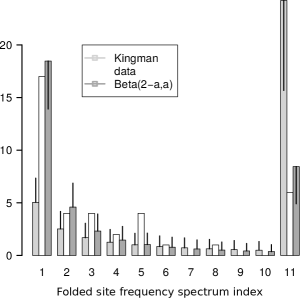
The folded freq. spectrum (white bars) of the data of [1] along with predictions of the Kingman coalescent (light-grey), and the Beta$(2-\hat{\alpha},\hat{\alpha})$-coalescent (dark-grey), where $\hat{\alpha}=1.5$ is the best fit estimated from the data according to [15]. Vertical lines represent the standard deviation; obtained for the Beta$(2-\hat{\alpha},\hat{\alpha})$-coalescent from $10^{5}$ iterations. Class ‘11’ represents the collated tail of the spectrum, from 11 to 1278/2.
Reproduced from [15, Fig. 11].

Figure 2.2.

Remark 2.3.

1. For a $\Lambda$-coalescent $\Pi$ there are analogous recursions for variances $\mathrm{Var}^{\Pi}\big{[}\xi^{(n)}_{i}\big{]}$ and covariances $\mathrm{Cov}^{\Pi}\big{[}\xi^{(n)}_{i},\xi^{(n)}_{j}\big{]}$, see [15, Theorem 2].

2. For the Kingman case, we have ${p^{(n),{\delta_{0}}}[k,b]}=\frac{\binom{n-b-1}{k-2}}{\binom{n-1}{k-1}}$ and $\mathbb{E}^{{\delta_{0}},\theta}=\left[\xi_{i}^{(n)}\right]=\frac{\theta}{i}$, as computed by Fu [29]. For general $\Lambda$-coalescents, no closed expressions for (2.5), (2.6) are known. However, the recursions can easily be solved numerically, even for $n$ in the hundreds.

3. The computation of the expected SFS through (2.6) is natural and conceptually appealing. We note however that there are now numerically more efficient alternatives, either via a spectral decomposition of the jump rate matrix of $Y$ as in Spence et al [63] or via an interpretation as a multivariate phase-type distribution as in Hobolth et al’s approach [42].

4. For $\Lambda$-coalescents with ‘strong $\alpha$-regular variation’ near $0$ (i.e., $\Lambda(dx)=f(x)dx$ with $f(x)\sim Ax^{1-\alpha}$ as $x\downarrow 0$ for some $A\in(0,\infty)$; this includes the $\mathrm{Beta}(2-\alpha,\alpha)$-coalescent from Example 1.2), [6, Thm. 8] shows $\xi^{(n)}_{i}\sim\frac{\theta}{2}n^{2-\alpha}C_{\alpha,i}$ a.s. with an explicit constant $C_{\alpha,i}$. However, the convergence in $n$ can be quite slow, see [11, Figure 8] and the discussion there.

5. Using similar arguments, one can derive recursion formulas for the expectation and covariances of the site frequency spectrum under $\Xi$-coalescents. See [10] and [63].

We see from (2.2.2) below and the following discussion that the SFS is closely allied to the distribution of branch lengths in coalescents. Asymptotic results for such lengths are a focus of the project by G. Kersting and A. Wakolbinger, described in this volume. E.g., see [20, 21] for the asymptotic behaviour of $B^{(n)}$ (the total branch length for sample size $n$) and of $B^{(n)}_{1}$ (the total branch length of the leaves) for very general coalescents and [19] for the fluctuations of $(B^{(n)}_{1}-\mathbb{E}[B^{(n)}_{1}])/n^{1-\alpha+1/\alpha}$ for $\mathrm{Beta}(2-\alpha,\alpha)$-coalescents with $1<\alpha<2$. For the Bolthausen-Sznitman coalescent and some ‘relatives,’ corresponding to $\alpha=1$, [20] obtain the asymptotic behaviour as $n\to\infty$ of $B^{(n)}_{i}$ for any $i\in\mathbb{N}$, see the article by Götz Kersting and Anton Wakolbinger in this volume.

The question of the theoretical identifiability of coalescents models from the expected site frequency spectrum has been treated in [63]. For example for $\Lambda$-coalescents, the first $n-2$ moments of the measure $\Lambda$ can be determined from the expected SFS with sample size $n$ and vice versa.

2.2. Inference methods based on the site-frequency spectrum

2.2.1. Inference of mutation rates and real-time embeddings.

When analysing data based on the SFS, one often needs to infer the underlying mutation rate first. Hence we begin this subsection with a brief discussion of this estimation and its consequences for the real-time embedding (assuming a “molecular clock”) of our coalescent models. Estimating $\theta$ (or $\theta/2$) is often done via the (analogue of) the Watterson estimator. Here, as pointed out e.g. in [27], it is important to understand that the choice of a multiple merger coalescent model $\Pi$ strongly affects this estimate. We illustrate this with an example. Assume w.l.o.g. for all multiple merger coalescents in question that the underlying coalescent measure $\Lambda$ is always a probability measure: This normalisation fixes the coalescent time unit as the expected time to the most recent common ancestor of two individuals sampled uniformly from the population.

Given an observed number of segregating sites $S$ in a sample of size $n$, a common (and unbiased) estimate $\hat{\theta}^{\Pi}$ of the scaled mutation rate $\theta$ in the coalescent scenario $\Pi$ is the Watterson estimate

(2.7) $$\hat{\theta}^{\Pi}:=\frac{2S}{\mathbb{E}^{\Pi}\big{[}B^{(n)}\big{]}},$$

where again $\mathbb{E}^{\Pi}\big{[}B^{(n)}\big{]}$ is the expectation of the total tree length $B^{(n)}$ of an ($n$-) coalescent model $\Pi$. One can compute for example $\mathbb{E}^{\Pi}\big{[}B^{(n)}\big{]}=\sum_{k=1}^{n}kg(n,k)$ with the Green function $g(n,k)$ from (2.3).

Now with the estimate $\hat{\theta}^{\Pi}$, given knowledge of the substitution rate $\hat{\mu}$ per year at the locus under consideration, one can obtain an approximate real-time embedding of the coalescent history via

(2.8) $${\rm coal.\ time\ unit}\times\frac{\hat{\theta}^{\Pi}}{2}\approx{\rm year}\times\hat{\mu}.$$

cf. [64, Section 4.2], which of course depends on the law $\mathbb{P}\hskip 0.5pt^{\Pi}$ of the $\Pi$-coalescent via the expected value $\mathbb{E}^{\Pi}\big{[}B^{(n)}\big{]}$. See also [68] for a study of the related concept of ‘effective population size.’

Given a Cannings population model of fixed size $N$ as discussed in Section 1.3, let $c_{N}$ be the probability that two gene copies, drawn uniformly at random and without replacement from a population of size $N,$ derive from a common parental gene copy in the previous generation. While for the usual haploid Wright-Fisher model $c_{N}=1/N$, in the class (B) from Section 1.3, $c_{N}$ is proportional to $1/N^{\alpha-1}$, for $1<\alpha\leqslant 2$. By the limit theorem for Cannings models of [50], one coalescent time unit corresponds to approximately $1/c_{N}$ generations in the original model with population size $N$. Thus the mutation rate $\tilde{\mu}$ at the locus under consideration per individual per generation must be scaled with $1/c_{N}$, and the relation between $\tilde{\mu}$, the coalescent mutation rate $\theta^{\Pi}/2$ and $c_{N}$ is then given by the (approximate) identity $c_{N}\approx 2\tilde{\mu}/\theta^{\Pi}$. In particular, if a Cannings model class (and thus $c_{N}$ as a function of $N$) is given, the ‘effective population size’ $N$ can then be estimated.

2.2.2. Approximate likelihood functions based on the SFS

Since mutations in our models occur as a Poisson process along the branches of a coalescent tree, for $\underline{k}=(k_{1},k_{2},\dots,k_{n-1})$ with $|\underline{k}|=\sum_{i=1}^{n-1}k_{i}=s$, the true likelihood function is

$$L\left((\Pi,\theta),\underline{k}\right) =\mathbb{P}\hskip 0.5pt^{\Pi,\theta}\big{\{}\xi^{(n)}_{i}=k_{i}^{(n)},i\in[n-1]\big{\}}=\mathbb{E}^{\Pi}\Bigg{[}\prod_{i=1}^{n-1}e^{-\frac{\theta}{2}B^{(n)}_{i}}\frac{(\theta B^{(n)}_{i}/2)^{k_{i}}}{k_{i}!}\Bigg{]}$$

(2.9) $$=\mathbb{E}^{\Pi}\Bigg{[}e^{-\theta B^{(n)}/2}\frac{(\theta B^{(n)}/2)^{s}}{s!}\cdot\frac{s!}{k_{1}!\cdots k_{n-1}!}\prod_{i=1}^{n-1}\bigg{(}\frac{B_{i}^{(n)}}{B^{(n)}}\bigg{)}^{k_{i}}\Bigg{]}$$

where $B_{i}^{(n)}$ is the random length of branches subtending $i\in[n-1]$ leaves and $B^{(n)}=B_{i}^{(n)}+\cdots+B_{n-1}^{(n)}$ is the total branch length of the $n$-coalescent tree $\Pi$. (2.2.2) is in general not expressible as a simple formula involving the coalescent parameters; it is in principle straightforwardly approximable via a ‘naive’ Monte Carlo approach but this is computationally very expensive even for moderate sample sizes. We note that Sainudiin and Véber [58] implement a clever approach to computing the expectation in (2.2.2) via importance sampling in the case of the Kingman coalescent (including variable population size and geographic structure); as far as we know, there is currently no study analogous to [58] that would include multiple merger coalescents.

Let us discuss an approximate likelihood function based on the so-called ‘fixed-$s$-method’. The idea is to treat the observed number of segregating sites as a fixed parameter $s\in\mathbb{N}$, not as (realisation of a) random variable $S$. This approximation appears quite common in the population genetics literature, see [27] and references there. Consider

(2.10) $$\mathbb{E}^{\Pi}\Bigg{[}\frac{s!}{k_{1}^{(n)}!\cdots k_{n-1}^{(n)}!}\prod_{i=1}^{n-1}\bigg{(}\frac{B_{i}^{(n)}}{B^{(n)}}\bigg{)}^{k_{i}^{(n)}}\Bigg{]},$$

(i.e., we take only the last term inside the expectation in (2.2.2)), this corresponds to uniformly and independently throwing $s$ mutations on the coalescent tree. An approximation is

(2.11) $$L(\Pi,\underline{k}^{(n)},s)\approx\frac{s!}{k_{1}^{(n)}!\cdots k_{n-1}^{(n)}!}\prod_{i=1}^{n-1}\big{(}\varphi^{\Pi,(n)}_{i}\big{)}^{k_{i}^{(n)}}$$

where we replaced the random quantities $B_{i}^{(n)}/B^{(n)}$ in (2.10) by the expected normalised branch lengths

(2.12) $$\varphi^{\Pi,(n)}_{i}=\mathbb{E}^{\Pi}[B_{i}^{(n)}]/\mathbb{E}^{\Pi}[B^{(n)}].$$

Equation (2.11) motivates the following family of ‘approximate’ (in a twofold sense: regarding both fixing $s$ and exchanging expectation of a fraction with a fraction of expectations) likelihood functions

$$\widetilde{L}(\Pi,\underline{\xi}^{(n)};s) =\prod_{i=1}^{n-1}e^{-\frac{\hat{\theta}(\Pi,s)}{2}\mathbb{E}^{\Pi}[B^{(n)}]\varphi_{i}^{\Pi,(n)}}\frac{\big{(}\frac{\hat{\theta}(\Pi,s)}{2}\mathbb{E}^{\Pi}[B^{(n)}]\varphi_{i}^{\Pi,(n)}\big{)}^{\xi^{(n)}_{i}}}{\xi^{(n)}_{i}!}$$

(2.13) $$=\prod_{i=1}^{n-1}e^{-s\varphi_{i}^{\Pi,(n)}}\frac{(s\varphi_{i}^{\Pi,(n)})^{\xi^{(n)}_{i}}}{\xi^{(n)}_{i}!}$$

where $\hat{\theta}(\Pi,s)=2s/\mathbb{E}^{\Pi}[B^{(n)}]$ is the Watterson estimator for the mutation rate under a $\Pi$-coalescent with $n$ leaves when $S=s$ segregating sites are observed, recall (2.7). In (2.2.2), we view $s$ as a parameter rather than as observed data, noting that $\widetilde{L}$ is well defined even if $|\underline{\xi}^{(n)}|\neq s$.

Note that for a principled approach to remove the dependence on the ‘nuisance parameter’ $\theta$, one could follow [4]. However, this is computationally very costly in the context of MMC’s and we do not pursue it here. For further discussion see [27].

(2.2.2) is a practical starting point for testing and parameter inference for multiple merger coalescent models, in particular this can be evaluated (and optimised) numerically very easily even for large sample sizes $n\gg 1$.

Let us also remark that (2.12) can also be the starting point for inference based on minimum-distance statistics, see [15].

2.3. Can one distinguish population growth from multiple merger coalescents?

We now employ the approximate likelihood functions from the previous section to construct a likelihood-ratio test for model selection. While this method has also been employed to select between various $\Xi-$coalescent models (see [11]), it can also be used to distinguish between different ‘evolutionary forces’ leading to non-Kingman-like variability in the SFS.

As an example, we discuss a scenario where the underlying population in question has undergone an exponential population increase as in [27]. Consider a haploid Wright-Fisher model with population size $N$ at generation $r=0$ and size $N(r)=N(1+\beta/N)^{-r}$ in generation $r$ before the present. This is in fact a special case of the set-up in [45] and we obtain in the limit, by speeding up time with a factor $N$ as usual, a Kingman-coalescent with exponentially growing coalescence rates $\nu(s)=e^{\beta s}$. Such a time-changed Kingman coalescent satisfies equation (2.2).

A population which has undergone a recent rapid increase should produce an excess of singletons in the SFS compared to model (K), which is a pattern also observed for Beta-coalescents. Similarly, Tajima’s $D$ (a classical test statistic in the Kingman context, see [67, Section 4.3]) would tend to be significantly negative under both model classes.

Our aim is to construct a statistical test to distinguish between the model classes ${\tt(E)}$ and ${\tt(B)}$ (which intersect exactly in ${\tt(K)}$). In order to distinguish ${\tt(E)}$ from ${\tt(B)}$, based on an observed site-frequency spectrum $\underline{\xi}^{(n)}$ with sample size $n$ and $S=|\underline{\xi}^{(n)}|$ segregating sites, a natural approach is to construct a likelihood-ratio test.

Suppose our null-hypothesis $H_{0}$ is presence of recent exponential population growth $({\scalebox{0.8}{\tt E}})$ with (unknown) parameter $\beta\in[0,\infty)$, and we wish to test it against the alternative $H_{1}$ hypothesis of a multiple merger coalescent, say, the Beta$(2-\alpha,\alpha)$-coalescent $(\scalebox{0.8}{\tt B})$ for (unknown) $\alpha\in[1,2]$, where $\beta=0$ and $\alpha=2$ correspond to the Kingman coalescent. The coalescent mutation rate $\theta$ is not directly observable, but plays the role of a nuisance parameter. By fixing $S=s$ and treating it as a parameter of our test, we may consider the pair of hypotheses

(2.14) $$H^{s}_{0}\,:\,\Pi\in\Theta_{s}^{\scalebox{0.8}{\tt E}}:=\big{\{}\text{Kingman coal., growth parameter }\beta:\beta\in[0,\infty)\big{\}}\vspace{-1ex}$$

and

(2.15) $$H^{s}_{1}\,:\,\Pi\in\Theta_{s}^{\scalebox{0.8}{\tt B}}:=\big{\{}\text{Beta$(2-\alpha,\alpha)$-coalescent}:\alpha\in[1,2]\big{\}}.$$

We can construct an ‘approximate likelihood-ratio’ test based on $L(\Pi,\underline{\xi}^{(n)},s)$ via

(2.16) $$\varrho_{(\scalebox{0.8}{\tt E},\scalebox{0.8}{\tt B};s)}(\underline{\xi}^{(n)}):=\frac{\sup\big{\{}L(\Pi,\underline{\xi}^{(n)},s),\,\Pi\in\Theta_{s}^{\scalebox{0.8}{\tt E}}\big{\}}}{\sup\big{\{}L(\Pi,\underline{\xi}^{(n)},s),\,\Pi\in\Theta_{s}^{\scalebox{0.8}{\tt B}}\big{\}}}$$

introduced in the previous section. Given a significance level $a\in(0,1)$ (say, $a=0.05$), let $\varrho^{*}_{(\scalebox{0.8}{\tt E},\scalebox{0.8}{\tt B};s)}(a)$ be the $a$-quantile of $\varrho_{(\scalebox{0.8}{\tt E},\scalebox{0.8}{\tt B};s)}(\underline{\xi}^{(n)})$ under E , chosen as the largest value so that

(2.17) $$\sup_{\Pi\in\Theta_{s}^{\scalebox{0.8}{\tt E}}}\mathbb{P}\hskip 0.5pt^{\Pi,s}\big{\{}\varrho_{(\scalebox{0.8}{\tt E},\scalebox{0.8}{\tt B};s)}(\underline{\xi}^{(n)})\leqslant\varrho^{*}_{(\scalebox{0.8}{\tt E},\scalebox{0.8}{\tt B};s)}(a)\big{\}}\leqslant a.$$

The decision rule that constitutes the ‘fixed-$s$-likelihood-ratio test’, given $s$ and sample size $n$, is

$$\hskip 14.22636pt\mbox{ reject $H_{0}^{s}$}\quad\iff\quad\varrho_{(\scalebox{0.8}{\tt E},\scalebox{0.8}{\tt B};s)}(\underline{\xi}^{(n)})\leqslant\varrho^{*}_{(\scalebox{0.8}{\tt E},\scalebox{0.8}{\tt B};s)}(a).$$

The corresponding power function of the test, that is, the probability to reject a false null-hypothesis, is given by

(2.18) $$G_{(\scalebox{0.8}{\tt E},\scalebox{0.8}{\tt B};s)}(\Pi)=\mathbb{P}\hskip 0.5pt^{\Pi}\{\varrho_{(\scalebox{0.8}{\tt E},\scalebox{0.8}{\tt B};s)}(\underline{\xi}^{(n)})\leqslant\varrho^{*}_{(\scalebox{0.8}{\tt E},\scalebox{0.8}{\tt B};s)}(a)\},\quad\Pi\in\Theta_{s}^{\scalebox{0.8}{\tt B}}.$$

Alternatively, even though $\widetilde{L}(\cdot,\cdot\,;s)$ from (2.2.2) is not literally a likelihood function of any model from $H_{0}^{s}\cup H_{1}^{s}$, we can consider the statistic $\widetilde{\varrho}_{(\scalebox{0.8}{\tt E},\scalebox{0.8}{\tt B})}(\underline{\xi}^{(n)})$, where we replace in (2.16) $L(\Pi,\underline{\xi}^{(n)},s)$ by $\widetilde{L}(\Pi,\underline{\xi}^{(n)},|\underline{\xi}^{(n)}|)$. For a given value of $s$, we can then (by simulations using the fixed-$s$-approach) determine approximate quantiles $\widetilde{\varrho}^{*}_{(\scalebox{0.8}{\tt E},\scalebox{0.8}{\tt B};s)}(a)$ associated with a significance level $a$ as in (2.17), and base our test on the criterion $\widetilde{\varrho}_{(\scalebox{0.8}{\tt E},\scalebox{0.8}{\tt B})}(\underline{\xi}^{(n)})\leqslant\widetilde{\varrho}^{*}_{(\scalebox{0.8}{\tt E},\scalebox{0.8}{\tt B};s)}(a)$. Similarly, the (approximate) power function

(2.19) $$\widetilde{G}_{(\scalebox{0.8}{\tt E},\scalebox{0.8}{\tt B};s)}=\mathbb{P}\hskip 0.5pt^{\Pi}\{\widetilde{\varrho}_{(\scalebox{0.8}{\tt E},\scalebox{0.8}{\tt B};s)}(\underline{\xi}^{(n)})\leqslant\widetilde{\varrho}^{*}_{(\scalebox{0.8}{\tt E},\scalebox{0.8}{\tt B};s)}(a)\}$$

for $\Pi\in\Theta_{s}^{\scalebox{0.8}{\tt B}}$ can be estimated using simulations. See the discussion in [27] and in particular Figure 2 there (a part of which we reproduce in Figure 2.3 below). For example, if the ‘truth’ was a Beta$(2-\alpha,\alpha)$-coalescent with $\alpha=1.5$, the power of a test of this form with significance level $5\%$ to reject $H_{0}^{s}$ (the null hypothesis of a Kingman model with exponential growth) based on a (single-locus) sample of size $n=500$ would be about $75\%$. Note that the power is reasonably high for $\alpha\leqslant 1.5$, say, but decays to the nominal level as $\alpha\to 2$. The boundary case $\alpha=2$ in the class of Beta$(2-\alpha,\alpha)$-coalescents is the Kingman coalescent, after all.

Figure 2.3. Estimate of $\widetilde{G}_{(\scalebox{0.8}{\tt E},\scalebox{0.8}{\tt B};s)}$ from (2.19) based on (2.2.2) as a function of $\alpha$ with $n=500$ and $s=50$. The symbols denote the size of the test, cf. legend. The hypotheses are discretised to $\Theta_{s}^{{\scalebox{0.8}{\tt E}}}=\{\beta:\beta\in\{0,1,2,\ldots,10,20,\ldots,1000\}\}$ and $\Theta_{s}^{\scalebox{0.8}{\tt B}}=\{\alpha:\alpha\in\{1,1.025,\ldots,2\}\}$. Here, the Beta$(2-\alpha,\alpha)$-coalescent is the alternative. Image reproduced from [27, Figure 2].

3. Multiple loci, diploidy and $\Xi$-coalescents

3.1. A diploid bi-parental multi-locus model

We model a population of $N$ diploid individuals. Each carries two chromosome copies, and each chromosome consists of $L$ loci. In a reproduction event, two randomly chosen parents produce a random number $\Psi^{(N)}$ of offspring, and these replace as many randomly chosen individuals; $\Psi^{(N)}$ is drawn afresh for each event. Each child inherits one (possibly recombined) chromosome from each parent according to the Mendelian laws; we assume that during meiosis, a crossover recombination between locus $\ell$ and $\ell+1$ happens with probability $r_{\ell}^{(N)}$ for $\ell\in[L-1]$. See Figure 3.1 for an illustration.

Example 3.1.

For a concrete example, assume that $\mathbb{P}\hskip 0.5pt(\Psi^{(N)}=\lceil\psi N\rceil)=c/N^{2}$ and $\mathbb{P}\hskip 0.5pt(\Psi^{(N)}=1)=1-c/N^{2}$ with $\psi\in(0,1)$, $c>0$. This leads to model (xEW).

Let $c_{N}:=\mathbb{E}\left[\Psi^{(N)}(\Psi^{(N)}+3)/N(N-1)\right]$ (this $4\times$ the pair coalescence probability for two randomly chosen chromosomes) and assume that

(3.1) $$\frac{c_{N}}{\mathbb{E}\left[\Psi^{(N)}/N\right]}=\frac{\mathbb{E}\left[\Psi^{(N)}(\Psi^{(N)}+3)\right]}{(N-1)\mathbb{E}\left[\Psi^{(N)}\right]}\mathop{\longrightarrow}_{N\to\infty}0$$

(which implies that also $c_{N}\to 0$) and that there exists a probability measure $\Lambda$ on $[0,1]$ such that

(3.2) $$\frac{1}{c_{N}}\mathbb{P}\hskip 0.5pt\left\{\Psi^{(N)}>Nx\right\}\mathop{\longrightarrow}_{N\to\infty}\int_{(x,1]}\frac{1}{y^{2}}\Lambda(dy)$$

for all continuity points $x\in(0,1]$ of $\Lambda$. Furthermore

(3.3) $$r_{\ell}^{(N)}\sim\frac{c_{N}}{4\mathbb{E}\left[\Psi^{(N)}/N\right]}r^{(\ell)}\quad\text{as}\;N\to\infty$$

with fixed $r_{\ell}\in[0,\infty)$ for $\ell=1,\dots,L-1$.

Remark 3.2.

Note that $\mathbb{E}\left[\Psi^{(N)}/N\right]$ is the probability that (after a given reproduction event) a randomly chosen individual from the current population is a child. (3.1) then ensures that ‘separation of time scales’ occurs: The ‘short’ time-scale $1/\mathbb{E}\left[\Psi^{(N)}/N\right]$ on which sampled chromosomes paired in the same individual disperse into two different individuals carrying only one sampled chromosome each is much smaller than the ‘long’ time-scale $1/c_{N}$ over which we observe non-trivial ancestral coalescences. This lies ‘behind’ Proposition 3.3 below.

For the classification of general diploid models (in the single-locus context), we refer to [9], see also the article by Anja Sturm in this volume.

$\begin{array}[]{c}\mbox{\small time}\\ \uparrow\end{array}$

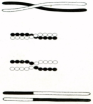
Figure 3.1. Schematic illustrations of the population model described in Section 3.1. Top left: $\Psi^{(N)}$ children of a single pair are created. Bottom left: Transmission of genetic information to the $\Psi^{(N)}$ children (which can include recombination). Right: A possible recombination event in producing a child. Far right: Schematic illustration of crossing over (an important step in the biochemical mechanism of recombination), adapted from Thomas Hunt Morgan, A Critique of the Theory of Evolution, Princeton University Press, 1916.

3.2. The $\Xi$-ancestral recombination graph

Consider a sample of $n$ chromosomes (which could be taken from $n/2$ sampled individuals, say), each of which carries $L$ loci. We need some notation to describe the ancestral states: A possible configuration has the form $\zeta=\{C_{1},C_{2},\dots,C_{b}\}$ with $b\in[n]$, where $C_{i}=(\widetilde{C}_{i,1},\widetilde{C}_{i,2},\dots,\widetilde{C}_{i,L})$ with $\widetilde{C}_{i,1},\dots,\widetilde{C}_{i,L}\subset[n]$ and not all $=\emptyset$ such that for $\ell=1,\dots,L$ we have $\bigcup_{i=1}^{b}\widetilde{C}_{i,\ell}=[n]$ and for $i\neq i^{\prime}$, $\widetilde{C}_{i,\ell}\cap\widetilde{C}_{i^{\prime},\ell}=\emptyset.$ $\widetilde{C}_{i,\ell}$ contains the indices of those samples for which the chromosome $C_{i}$ in the current configuration is ancestral at the $\ell$-th locus. Thus, for each locus $\ell$, $\{\widetilde{C}_{1,\ell},\dots,\widetilde{C}_{b,\ell}\}$ is a partition of $[n]$ (with a grain of salt: it may contain $\emptyset$’s). We write $\mathcal{A}$ for the set of all configurations of this form. We remark that in order to properly describe the dynamics of ancestral configurations for finite population size $N$, $\mathcal{A}$ is in fact not completely sufficient and has to be ‘enriched’ by information about the grouping of ancestral chromosomes into diploid individuals. However, because of the separation of time scales described in Remark 3.2, this becomes irrelevant for the limit process. We will not go into details here and refer to [11].

From $\zeta\in\mathcal{A}$, possible transitions lead to

$$\mathsf{pairmerge}_{i_{1},i_{2}}(\zeta) =\big{\{}C_{1},\dots,C_{i_{1}-1},\widehat{C}_{i_{1}},C_{i_{1}+1},\dots,C_{i_{2}-1},C_{i_{2}+1},\dots,C_{b}\big{\}}$$

with $$\widehat{C}_{i_{1}}=\left(\widetilde{C}_{i_{1},1}\cup\widetilde{C}_{i_{2},1},\dots,\widetilde{C}_{i_{1},\ell}\cup\widetilde{C}_{i_{2},\ell}\right) C_{i_{1}} C_{i_{2}}$$, a merger of the pair and ,

$$\mathsf{groupmerge}_{J}(\zeta) =\big{\{}\overline{C}_{1},\overline{C}_{2},\overline{C}_{3},\overline{C}_{4},\,C_{j},j\in[b]\setminus(J_{1}\cup J_{2}\cup J_{3}\cup J_{4})\big{\}}$$

with $$J_{1},\dots,J_{4}\subset[b] |J_{i}|\geqslant 3 |J_{i}|\geqslant 2 \overline{C}_{m}=\Big{(}\bigcup_{i\in J_{m}}\widetilde{C}_{i,1},\bigcup_{i\in J_{m}}\widetilde{C}_{i,2},\dots,\bigcup_{i\in J_{m}}\widetilde{C}_{1,\ell}\Big{)} m=1,2,3,4$$ pairwise disjoint and at least one or at least two of the . Here, for , a simultaneous multiple merger in (up to) four groups, and

$$\mathsf{recomb}_{i,\ell}(\zeta) =\left\{C_{1},\dots,C_{i-1},C_{i}^{\prime},C_{i}^{\prime\prime},C_{i+1},\dots,C_{b}\right\}$$

with $C_{i}^{\prime}=(\widetilde{C}_{i,1},\widetilde{C}_{i,2},\dots,\widetilde{C}_{i,\ell},\emptyset,\dots,\emptyset)$ and $C_{i}^{\prime}=(\emptyset,\dots,\emptyset,\widetilde{C}_{i,\ell+1},\widetilde{C}_{i,\ell+2},\dots,\widetilde{C}_{i,L},)$, a recombination event splitting the $i$-th chromosome in the configuration between locus $\ell$ and locus $\ell+1$.

Note that as mentioned above, both in the $\mathsf{pairmerge}$ and the $\mathsf{groupmerge}$ operations, ‘empty’ entries $(\emptyset,\emptyset,\dots,\emptyset)$ may arise, which then need to be removed; see [11] for details.

The limiting genealogical process will then be a continuous-time Markov chain $\{\xi(t)\}_{t\geqslant 0}$ on $\mathcal{A}$ with generator matrix $q$ whose off-diagonal elements are given by

(3.4) $$q_{\xi,\xi^{\prime}}=\begin{cases}C_{\beta;2}&\text{if}\;\xi^{\prime}=\mathsf{pairmerge}_{j_{1},j_{2}}(\xi)\\ r^{(\ell)}&\text{if}\;\xi^{\prime}=\mathsf{recomb}_{j,\ell}(\xi)\\ C_{\beta;|J|}&\text{if}\;\xi^{\prime}=\mathsf{groupmerge}_{J_{1},J_{2},J_{3},J_{4}}(\xi)\\ 0&\text{for all other $\xi^{\prime}\neq\xi$}\end{cases}$$

where $C_{\beta;|J|}:=C_{\beta;|J_{1}|,|J_{2}|,|J_{3}|,|J_{4}|;\beta-(|J_{1}|+|J_{2}|+|J_{3}|+|J_{4}|)}$ and

(3.5) $$C_{b;k;s} =\Lambda(\{0\})\delta_{\{r=1,k_{1}=2\}}+4\sum_{l=0}^{s\wedge(4-r)}{s\choose l}\tfrac{(4)_{r+l}}{4^{|k|+l}}\cdot\int_{(0,1]}x^{|k|+l}(1-x)^{s-l}\frac{1}{x^{2}}\Lambda(dx)$$

with $k=(k_{1},\ldots,k_{r})$, $|k|=k_{1}+\cdots+k_{r}$. The path of $\{\xi_{t}\}$ can be visualised as a random network, see Figure 3.2 for an illustration.

Proposition 3.3 ([11, Theorem 1.3]).

Let $\{\xi^{n,N}(m),m\geqslant 0\}$ be the ancestral process of a sample of $n$ chromosomes in a population of size $N$ with offspring laws $\mathcal{L}(\Psi^{(N)})$ satisfying (3.1) and (3.2), and assume the scaling relation (3.3).

(3.6) $$\{\xi^{n,N}(\lfloor 4t/c_{N}\rfloor)\}\longrightarrow\{\xi(t)\}\quad\mbox{ as }\quad N\to\infty,$$

where the process $\{\xi(t)\}$ is the Markov chain with generator matrix (3.4).

We refer to [11] for details, in particular the precise mode of convergence in (3.6) depending on whether or not the grouping of ancestral chromosomes into possibly ‘doubly marked individuals’ is taken into account.

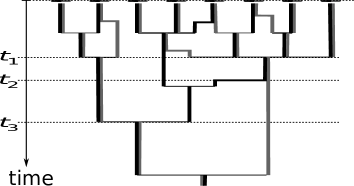
Figure 3.2. An illustration of the $\Xi$-ancestral recombination graph for two loci, with some transitions highlighted. At time $t_{1}$, a $\mathsf{groupmerge}$-event occurs. At time $t_{2}$, there is a $\mathsf{recomb}$-event and at time $t_{3}$, a $\mathsf{pairmerge}$-event.

3.3. Towards a full SMMC multilocus inference machinery

One can incorporate the (biologically important) effects of recombination, spatial subdivision, variable population size (e.g. growing populations), and/or (directional) selection into stochastic models for populations with highly skewed offspring distributions and derive corresponding (limiting) models for the joint genealogy of an $n$-sample observed at $L$ (possibly recombining) loci. The ‘full complexity’ model is then a ‘structured $\Xi$-ancestral selection recombination graph.’ While in principle highly relevant in view of today’s large scale datasets, an explicit description of the resulting full sampling distributions seems out of reach at present. One can however make progress on statistical questions by employing low-dimensional summary statistics. One approach, inspired by the results from Section 2.2 is to use suitable lumpings of the normalised site frequency spectra and average these over the observed loci: Let

(3.7) $$\zeta_{1}(\ell):=\frac{\xi_{1}(\ell)}{|\xi(\ell)|},\quad\overline{\zeta}_{k}(\ell):=\sum_{j=k}^{n-1}\frac{\xi_{j}(\ell)}{|\xi(\ell)|}$$

be the proportion of singletons and the proportion of mutations visible in more than $k\geqslant 2$ copies at the $\ell$-th locus, respectively.

(3.8) $$\left(\zeta_{1},\overline{\zeta}_{k}\right):=\frac{1}{L}\sum_{\ell=1}^{L}\left(\zeta_{1}(\ell),\overline{\zeta}_{k}(\ell)\right)$$

is a two-dimensional summary of the data whose distribution under a given coalescent model $\Pi$ with mutation parameter $\theta>0$

(3.9) $$L\left(\Pi,\theta,(z_{1},\overline{z}_{k})\right):=\mathbb{P}\hskip 0.5pt^{\Pi,\theta}\Big{(}\left(\zeta_{1},\overline{\zeta}_{k}\right)=(z_{1},\overline{z}_{k})\Big{)}$$

is generally not known explicitly, but $\left(\zeta_{1},\overline{\zeta}_{k}\right)$ can be simulated readily under $(\Pi,\theta)$. Then the function $(z_{1},\overline{z}_{k})\mapsto L\left(\Pi,\theta,(z_{1},\overline{z}_{k})\right)$ from (3.9) can be approximated by a kernel estimator based on $M$ independent replicates:

(3.10) $$\widehat{L}\left(\Pi,\theta,(z_{1},\overline{z}_{k})\right):=\frac{1}{Mh}\sum_{m=1}^{M}K\left(\frac{1}{h}\left((\zeta_{1},\overline{\zeta}_{k})-\big{(}\zeta_{1},\overline{\zeta}_{k}\big{)}(m)\right)\right)$$

where $\big{(}\zeta_{1},\overline{\zeta}_{k}\big{)}(m)$ is the value of (3.8) computed from the $m$-th simulation and $K$ the kernel function (e.g. a Gaussian) with bandwidth $h>0$. Given (3.10), testing and model selection analogous to Section 2.3 can now be based on the approximate likelihood ratio statistic

(3.11) $$\frac{\sup_{(\Pi,\theta)\in\Theta_{0}}\widehat{L}\left(\Pi,\theta,(z_{1},\overline{z}_{k})\right)}{\sup_{(\Pi,\theta)\in\Theta_{1}}\widehat{L}\left(\Pi,\theta,(z_{1},\overline{z}_{k})\right)}$$

where of course the critical value for a test of given size has to be determined by simulations. In practice, one can alleviate the two-dimensional optimisation problem in (3.11) by plugging in the Watterson estimator $\theta=\hat{\theta}^{\Pi}$ from (2.7) given coalescent model $\Pi$.

This approach is pursued in [47], with promising initial results, see the discussion there and also Figure 3.3 below. It can also be extended to include the effects of selection, variable population sizes and spatial structure, see [48] for steps in this direction. Note that this is akin to approximate Bayesian computations (ABC), whose rôle in analyses of datasets in multiple merger contexts is described in the article by Fabian Freund in this volume.

Intuitively, although even unlinked loci are not independent under the skewed offspring distribution models from Section 3.2 (as observed in [11]), averaging over many loci does reduce sampling variability and is justified because the multiple merger mechanism affects all loci in the same way. This is in fact a distinguishing feature that explains why multi-locus data is useful to distinguish skewed offspring distributions from selective sweeps: The latter would only affect one locus at a time.

Figure 3.3. The empirical distribution of $(\zeta_{1},\overline{\zeta}_{k})$ from (3.8) is quite different under a Kingman coalescent with exponential growth (solid contours) compared to a 4-fold Beta coalescent (xB) (dashed contours). Here, the sample size is $n=100$, each sample considered at $L=23$ loci, with cutoff parameter $k=15$. Parameter values ($\alpha$ for the 4-fold Beta($2-\alpha,\alpha$) coalescent, $\beta$ for the exponential growth rate) are as shown. The contour lines are based on 5000 simulated replicates for each parameter choice: For this, mutation rates $\theta$ were chosen so that the expected number of segregating sites per locus equalled $s_{\text{expect}}^{(n),\Pi}=10,20,30,40,50$ (cf. Equ. (2.7)), with 1000 replicates per value of $\theta$. The pictures for a fixed value of $s_{\text{expect}}^{(n),\Pi}$ are almost indistinguishable from the one shown. The contours were computed using R [53] and the function kde from the contributed R-package ks [24], with default values for the bandwiths. They correspond to regions containing respectively 20%, 40%, 60%, 80% and 95% of the simulated points.

The software used for this study is available under https://github.com/JereKoskela/Beta-Xi-Sim. Furthermore, software for simulation and analysis of datasets in (S)MMC contexts can be found on Bjarki Eldon’s homepage http://page.math.tu-berlin.de/~eldon/programs.html.

4. Discussion - Are they really out there?

In the previous sections, we outlined population models and evolutionary scenarios which invite genealogical modelling via (S)MMC processes. Further, we presented some paradigmatic statistical tools for inference and model selection for (S)MMC processes, and our hope is that this could pave at least some of the way towards an answer to initial question [28] whether (S)MMC coalescents are really more adequate null-models for real populations exhibiting highly skewed offspring distributions (or other forces leading to an ‘effective skew’, such as selective sweeps, severe bottlenecks etc.).

One of our main take-home messages is that the statistical power of such inference methods is usually much higher in (diploid) multi-locus setups rather than in (haploid) single locus scenarios. However, it is the latter scenario in which MMC based inference methods have so far been applied in practice. For example, the results in [64] indicate that data generated under a Beta-coalescent can provide a better fit to observed genetic variability in Atlantic cod mitochondrial (thus haploid) DNA sequence data. In the cited article, it is also discussed in how far different underlying coalescent models lead to different estimates for the real-time most recent common ancestor of the sample. To some degree, it appears also possible to distinguish different evolutionary scenarios such as a recent increase in population size, leading to a time-changed Kingman coalescent, from other coalescent scenarios, as reviewed in in Sections 2.3 and 3.3.

A very recent further study involving virus data (influenza) is [55], which employs purely-atomic MMCs (of class (EW)), again in a haploid setup. The authors here come to the conclusion that the (EW) coalescent can provide a “much more accurate neutral null model” in certain types of organisms including viruses and bacteria. However, the study seems to be restricted to a relatively small class of MMCs.

We expect that a real test for the above methods will be in the framework of diploid multi-locus setups. A very interesting step in this direction is the recent work of Rice, Novembre and Desai [54] who propose a statistic based on the joint site frequency spectrum at two loci. This approach does not explicitly model multi-locus dynamics including recombination, but it can (quite straightforwardly) be scaled up to analyse genome-wide genetic variability and, as shown in [54], does shed a very interesting light on a Zambian population of fruit flies (Drosophila melanogaster). Furthermore, in this context, it is rather satisfying to see that the funding of the Icelandic Grant of Excellence “Population genomics of highly fecund codfish” has recently been awarded jointly to Árnason, Halldórsdóttir, Etheridge, and Stephan. Our hope is that this project will provide and analyse the necessary data on which the full multi-locus machinery can be tested. We will be curious to observe the outcomes.

Acknowledgements. The authors would like to thank Iulia Dahmer, Frederik Klement and Timo Schlüter for carefully reading the manuscript and for their helpful comments. We also thank Iulia Dahmer for her help in producing Figure 3.3 and two anonymous referees for their insightful comments which helped to improve the presentation of this article.

References

- [1] E. Árnason, Mitochondrial Cytochrome b DNA Variation in the High-Fecundity Atlantic Cod: Trans-Atlantic Clines and Shallow Gene Genealogy, Genetics 166 (2004), 1871–1885.
- [2] E. Árnason and K. Halldórsdóttir, Nucleotide variation and balancing selection at the Ckma gene in Atlantic cod: analysis with multiple merger coalescent models, PeerJ 3:e786 http://dx.doi.org/10.7717/peerj.786.
- [3] N. Barton, A. Etheridge and A. Véber, A new model for evolution in a spatial continuum, Electron. J. Probab. 15 (2010), 162–216.
- [4] R. L. Berger and D. D. Boos, P values maximized over a confidence set for the nuisance parameter, J. Amer. Statist. Assoc. 89 (1994), 1012–1016.
- [5] N. Berestycki, Recent Progress in Coalescent Theory, Ensaios Matematicos 16 (2009), 1–193.
- [6] J. Berestycki, N. Berestycki and V. Limic, Asymptotic sampling formulae for -coalescents, Ann. Inst. Henri Poincaré Probab. Stat. 50 (2014), 715–731.
- [7] J. Berestycki, N. Berestycki and J. Schweinsberg, The genealogy of branching Brownian motion with absorption, Ann. Probab. 41 (2013), 527–618.
- [8] J. Bertoin and J.-F. Le Gall, Stochastic flows associated to coalescent processes, Probab. Theory Related Fields 126 (2003), 261–288.
- [9] M. Birkner, H. Liu and A. Sturm, Coalescent results for diploid exchangeable population models, Electron. J. Probab. 23 (2018), 1–44.
- [10] J. Blath, M. Cronjaeger, B. Eldon, and M. Hammer, The site-frequency spectrum associated with Xi-coalescents, Theoret. Population Biol. 10 (2016), 36–50.
- [11] M. Birkner, J. Blath and B. Eldon, An ancestral recombination graph for diploid populations with skewed offspring distribution, Genetics 193 (2013), 255–290.
- [12] M. Birkner and J. Blath, Computing likelihoods for coalescents with multiple collisions in the infinitely many sites model, J. Math. Biol. 57 (2008), 435–465.
- [13] M. Birkner, J. Blath, M. Möhle, M. Steinrücken, and J. Tams, A modified lookdown construction for the Xi-Fleming-Viot process with mutation and populations with recurrent bottlenecks, ALEA Lat. Am. J. Probab. Math. Stat. 6 (2009), 25–61.
- [14] M. Birkner, J. Blath, M. Capaldo, A. Etheridge, M. Möhle, J. Schweinsberg, and A. Wakolbinger, Alpha-stable branching and beta-coalescents, Electron. J. Probab. 10 (2005), 303–325.
- [15] M. Birkner, J. Blath and B. Eldon, Statistical properties of the site-frequency spectrum associated with Lambda-coalescents, Genetics 195 (2013), 1037–1053.
- [16] E. Bolthausen and A.-S. Sznitman, On Ruelle’s probability cascades and an abstract cavity method, Comm. Math. Phys. 197 (1998), 247–276.
- [17] C. Cannings, The latent roots of certain Markov chains arising in genetics: a new approach, I. Haploid models. Adv. in Appl. Probab. 6 (1974), 260–290.
- [18] M. M. Desai, A. M. Walczak and D. S. Fisher, Genetic diversity and the structure of genealogies in rapidly adapting populations, Genetics 193 (2013), 565–585.
- [19] I. Dahmer, G. Kersting and A. Wakolbinger, The total external branch length of Beta-coalescents, Combin. Probab. Comput. 23 (2014), 1010–1027.
- [20] C. Diehl and G. Kersting, Tree lengths for general -coalescents and the asymptotic site frequency spectrum around the Bolthausen-Sznitman coalescent, preprint, arXiv:1804.00961 (2018).
- [21] C. Diehl and G. Kersting, External branch lengths of -coalescents without a dust component, preprint, arXiv:1811.07653 (2018).
- [22] P. Donnelly and T. Kurtz, A countable representation of the Fleming-Viot measure-valued diffusion, Ann. Probab. 24 (1996), 698–742.
- [23] P. Donnelly and T. Kurtz, Particle representations for measure-valued population models, Ann. Probab. 27 (1999), 166–205.
- [24] T. Duong, ks: Kernel Smoothing, R package version 1.11.5 (2019), https://CRAN.R-project.org/package=ks
- [25] R. Durrett, Probability Models for DNA Sequence Evolution, 2nd ed., Springer, 2008.
- [26] R. Durrett and J. Schweinsberg, A coalescent model for the effect of advantageous mutations on the genealogy of a population, Stochastic Process. Appl. 115 (2005), 1628–1657.
- [27] B. Eldon, M. Birkner, J. Blath, and F. Freund, Can the site-frequency spectrum distinguish exponential population growth from multiple-merger coalescents? Genetics 199 (2015), 841–856.
- [28] B. Eldon and J. Wakeley, Coalescent processes when the distribution of offspring number among individuals is highly skewed, Genetics 172 (2006), 2621–2633.
- [29] Y. X. Fu, Statistical properties of segregating sites, Theoret. Population Biol. 48 (1995), 172–197.
- [30] J. Felsenstein, M. K. Kuhne, J. Yamato and P. Beerli, Likelihoods on coalescents: a Monte Carlo sampling approach to inferring parameters from population samples of molecular data, In Statistics in Molecular Biology and Genetics, IMS Lecture Notes, vol. 33, 1999.
- [31] A. González Casanova, V. Miró Pina and A. Siri-Jégousse, The Symmetric Coalescent and Wright-Fisher models with bottlenecks, preprint, arXiv:1903.05642, 2019.
- [32] A. Greven, P. Pfaffelhuber and A. Winter, Convergence in distribution of random metric measure spaces: The -coalescent measure tree, Probab. Theory Related Fields 145 (2009).
- [33] A. Gnedin, A. Iksanov and A. Marynych, -coalescents: A survey, J. Appl. Probab. 51A (2014), 23–40.
- [34] J. Gillespie, Population genetics: a concise guide, Johns Hopkins Univ. Press, 1998.
- [35] R. C. Griffiths and P. Marjoram, An ancestral recombination graph, Progress in population genetics and human evolution, 257–270, missingIMA Vol. Math. Appl. 87, Springer, 1997.
- [36] R. C. Griffiths and S. Tavaré, The age of a mutation in a general coalescent tree, Stoch. Models 14 (1998), 273–295.
- [37] S. Gufler, A representation for exchangeable coalescent trees and generalized tree-valued Fleming-Viot processes, Electron. J. Probab. 23 (2018), 1–42.
- [38] S. Gufler, Pathwise construction of tree-valued Fleming-Viot processes, Electron. J. Probab. 23 (2018), 1–58.
- [39] D. Gusfield, Efficient algorithms for inferring evolutionary trees, Networks 21 (1991), 19–28.
- [40] D. Hedgecock, Does variance in reproductive success limit effective population size of marine organisms?, pp. 123–134 in Genetics and Evolution of Aquatic Organisms, edited by A. R. Beaumont, Chapman & Hall, London, 1994.
- [41] D. Hedgecock and A. I. Pudovkin, Sweepstakes reproductive success in highly fecund marine fish and shellfish: a review and commentary, Bull. Mar. Sci. 87 (2011), 971–1002.
- [42] A. Hobolth, A. Siri-Jégousse and M. Bladt, Phase-type distributions in population genetics, preprint, arXiv:1806.01416, 2018.
- [43] R. R. Hudson, Properties of a neutral allele model with intragenic recombination, Theoret. Population Biol. 23 (1983), 183–201.
- [44] Thierry E. Huillet, Pareto genealogies arising from a Poisson branching evolution model with selection, J. Math. Biol. 68 (2014), 727–761.
- [45] I. Kaj, S. Krone, J. Appl. Probab. 40 (2003), 33–48.
- [46] J. F. C. Kingman, The coalescent, Stoch. Proc. Appl. 13 (1982), 235–248.
- [47] J. Koskela, Multi-locus data distinguishes between population growth and multiple merger coalescents, Stat. Appl. Genet. Mol. Biol. 17 (2018), 20170011.
- [48] J. Koskela and M. Wilke Berenguer, Robust model selection between population growth and multiple merger coalescents, Math. Biosci. 311 (2019), 1–12.
- [49] M. Möhle and H. Pitters, A spectral decomposition for the block counting process of the Bolthausen-Sznitman coalescent, Electron. Commun. Probab. 19 (2014), 11 pp.
- [50] M. Möhle and S. Sagitov, A classification of coalescent processes for haploid exchangeable population models, Ann. Probab. 29, 1547–1562.
- [51] R. A. Neher and O. Hallatschek, Genealogies of rapidly adapting populations, Proc. Natl. Acad. Sci. 110 (2013), 437–442.
- [52] J. Pitman, Coalescents with multiple collisions, Ann. Probab. 27 (1999), 1870–1902.
- [53] R Core Team, A language and environment for statistical computing, R Foundation for Statistical Computing, https://www.R-project.org/
- [54] D. P. Rice, J. Novembre and M. M. Desai, Distinguishing multiple-merger from Kingman coalescence using two-site frequency spectra, preprint, biorxiv:461517v1 (2018).
- [55] A. M. Sackman, R. Harris and J. D. Jensen, Inferring demography and selection in organisms characterized by skewed offspring distributions, Genetics 211 (2019), 1019–1028.
- [56] S. Sagitov, The general coalescent with asynchronous mergers of ancestral lines, J. Appl. Probab. 36 (1999), 1116–1125.
- [57] S. Sagitov, Convergence to the coalescent with simultaneous multiple mergers, J. Appl. Probab. 40 (2003), 839–854.
- [58] R. Sainudiin and A. Véber, Full likelihood inference from the site frequency spectrum based on the optimal tree resolution, Theor. Pop. Biol. 124 (2018), 1–15.
- [59] J. Schweinsberg, Coalescents with simultaneous multiple collisions, Electron. J. Probab. 5 1–50.
- [60] J. Schweinsberg, Coalescent processes obtained from supercritical Galton-Watson processes, Stochastic Process. Appl. 106 (2003), 107–139.
- [61] J. Schweinsberg, Rigorous results for a population model with selection I: evolution of the fitness distribution. Electron. J. Probab. 22 (2017), 1–94.
- [62] J. Schweinsberg, Rigorous results for a population model with selection II: genealogy of the population, Electron. J. Probab. 22 (2017), 1–54.
- [63] J. P. Spence, J. A. Kamm, Y. S. Song, The site frequency spectrum for general coalescents, Genetics 202 (2016), 1549–1561.
- [64] M. Steinrücken, M. Birkner and J. Blath. Analysis of DNA sequence variation within marine species using Beta-coalescents, Theoret. Population Biol. 87 (2013), 15–24.
- [65] M. Stephens and P. Donnelly, Inference in molecular population genetics, With discussion and a reply by the authors, J. R. Stat. Soc. Ser. B Stat. Methodol. 62 (2000), 605–655.
- [66] A. Tellier and C. Lemaire, Coalescence 2.0: a multiple branching of recent theoretical developments and their applications, Mol. Ecol. 23 (2014), 2637–2652.
- [67] J. Wakeley, Coalescent Theory: An Introduction. Roberts & Company Publishers, Greenwood Village, Colorado, 2008.
- [68] J. Wakeley and O. Sargsyan, Extensions of the Coalescent Effective Population Size, Genetics 181 (2009), 341–345.
- [69] G. A. Watterson, On the number of segregating sites in genetical models without recombination, Theoret. Population Biol. 7 (1975), 1539–1546.
Index
- ancestral recombination graph §3.2
- Beta-coalescent item (B), §2.3
- block-counting process of a coalescent §2.1
- branch lengths of a coalescent tree §2.1.2
- Cannings model §1.3
- coalescent
- diploid item (xEW), (xB), §3.1
- effective population size §2.2.1
- Eldon-Wakeley coalescent item (EW)
- infinitely-many-sites model §2
- Kingman coalescent item (K), §1.1
-
likelihood function §2.2.2
- approximate §2.2.2
-
likelihood-ratio text
- approximate §2.3
- multi-locus model §3.1
- multiple merger coalescent §1.2.1
- pair coalescence probability §2.2.1, §3.1
- Poisson-Dirichlet coalescent item (PD)
- population model §1.3
- Schweinsberg’s model item (B)
- sequence data §2
- Simultaneous multiple merger (SMMC) coalescent §1.2.2
- site-frequency spectrum §2
- -coalescent §1.2.1
- -ancestral recombination graph §3.2
- -coalescent §1.2.2