The geometry of passivity for quantum systems and a novel elementary derivation of the Gibbs state
Abstract
Passivity is a fundamental concept that constitutes a necessary condition for any quantum system to attain thermodynamic equilibrium, and for a notion of temperature to emerge. While extensive work has been done that exploits this, the transition from passivity at a single-shot level to the completely passive Gibbs state is technically clear but lacks a good over-arching intuition. Here, we reformulate passivity for quantum systems in purely geometric terms. This description makes the emergence of the Gibbs state from passive states entirely transparent. Beyond clarifying existing results, it also provides novel analysis for non-equilibrium quantum systems. We show that, to every passive state, one can associate a simple convex shape in a -dimensional plane, and that the area of this shape measures the degree to which the system deviates from the manifold of equilibrium states. This provides a novel geometric measure of athermality with relations to both ergotropy and –athermality.00footnotetext: ∗ NK and RA contributed equally to this paper. The ordering has been decided by random coin flip, generated on the IBM Q machine in conjunction with the von Neumann coin trick to reduce bias.
1 Introduction
The Gibbs state is a cornerstone of equilibrium statistical mechanics, and provides a rigorous notion of temperature for any quantum system. There are a range of justifications for this state, and each reveals different facets of thermodynamics. For example, it can be obtained from a micro-canonical ensemble derivation [1], where one posits an equal a priori probability distribution over energies for some large system and then proceeds to analyse the resultant marginal state on a much smaller subsystem. It can also be described from an inferential perspective, where one adopts a maximally unbiased description of the quantum system subject to known constraints – namely a maximum entropy construction [2, 3]. One highly active area of research is to determine the conditions under which a dynamically-evolving system tends towards an equilibrium state, and moreover one in which a notion of temperature emerges [4, 5, 6]. However, there is another route to the Gibbs state that is appealing in its physical simplicity, namely through the concept of passivity of quantum states [7, 8, 9]. This arose in the study of infinite-dimensional quantum systems, where one must adopt an algebraic description in order to rigorously describe features such as phase transitions [10].
Loosely speaking, passivity captures the inability of a quantum state to be used to ‘raise a weight’. The concept of passivity does not tell us when quantum systems dynamically equilibrate, instead it provides a simple characterisation of Gibbs states. This simplicity also makes it well-suited to exploring structural aspects of thermodynamics in quantum systems beyond equilibrium, and for elucidating the conceptual ingredients required for a notion of equilibrium to be established.
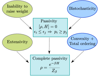
In recent times, passivity has received renewed attention. It has played a valuable role in studying the problem of work-extraction from non-equilibrium states [11, 12, 13, 14, 15], generalised Gibbs states [16, 17, 18, 19, 20] and quantum information-theoretic approaches to thermodynamics [21, 22, 23, 24, 25].
The original passivity analysis was in terms of algebras [7], and so did not lend itself to a widely accessible account. This was in part remedied by Lenard in 1978, who provided an analysis specialised to finite-dimensional quantum systems [8]. There have since been shorter and more compact passivity analyses, for example via the concept of ‘virtual temperatures’ [9]. While such derivations of the Gibbs state from passivity are technically clear, one might wish for a more intuitive perspective on the structure of passivity that makes the emergence of the Gibbs state entirely inevitable while suggesting natural extensions.
With this aim in mind, we present a novel geometric formulation of passivity. In particular, we show in Section 3.3 that every passive state of a quantum system can be associated to a simple convex shape in the -d plane. This convex shape naturally emerges in the macroscopic regime of many independent copies of the state, and its structure entirely encodes the deviation of the system from the manifold of equilibrium states. With this geometric notion, in Section 3.4 we show how the Gibbs state derivation becomes almost trivial, and that the area of the shape is a well-defined measure of the degree to which the state deviates from equilibrium. In Section 4.2, we show the area is monotonically non-increasing along so-called activation trajectories in the energy-entropy plane, and argue that it can supplement the traditional macroscopic equilibrium variables to capture the macroscopic non-equilibrium properties of a quantum system. We also demonstrate in Section 4.3 how the area relates to the concept of ergotropy [26], as well as the recently introduced notion of –athermality [27].
2 The core physical principles
We begin by making clear what physical notions we use and why they are either required or appealing conceptually. The two core components involved are the concepts of passivity and extensivity, which we now explain.
2.1 Passivity
The first core principle in our treatment is passivity, which is physically and operationally clear and fully deterministic. Two examples suffice to illustrate the main idea. First, consider a three-level atom with Hamiltonian in the following population-inverted state
| (1) |
By applying a unitary evolution to the system that deterministically swaps levels 1 and 3, we can lower the average energy of the system. In particular, the ‘passifying’ unitary transforms the state of the system to the new state :
| (2) |
The internal energy of the system has decreased by amount
| (3) |
which implicitly corresponds to work extraction. However, given the state in Eq. (2) the average energy cannot be lowered any further by any unitary. Therefore, there has been a maximal extraction of work from the quantum state with respect to any possible unitary evolution of the system, and the quantity in Eq. (3) corresponds to the ergotropy of [26]. Another example for the same Hamiltonian is given by the uniform superposition state
| (4) |
Given such an initial state it is possible to unitarily transform the system precisely to its ground state
| (5) |
where and is represented in the basis. Clearly, we cannot further lower the energy of this atomic system in its ground state via unitary evolution. States such as and , for which no further lowering of energy can occur through deterministic unitary transformations, are called passive. This is formalised by the following definition [7].
Definition 1.
A quantum state of a system with Hamiltonian is passive if
| (6) |
for all unitaries acting upon the system.
For simplicity, we restrict our attention to finite dimensional systems with bounded energies, although the notion of passivity extends to infinite dimensional systems [7]. In light of this definition, a natural question is: when exactly is a quantum state passive? The following theorem provides necessary and sufficient conditions for a finite-dimensional state being passive [8].
Theorem 2.
Consider a -dimensional quantum system with Hamiltonian , with eigenvalue decomposition . A state of that system is passive if and only if and, for eigenvalue decomposition , we have that implies for all and in .
See Appendix A for a majorization-based proof. Thus, passive states are precisely those which are block-diagonal in the energy eigenbasis with eigenvalues which are ‘anti-ordered’ with respect to the energies.
The definition of passivity does not invoke the full machinery of thermodynamics. It is a physical statement about the deterministic extraction of energy from a system. However, the notion is embedded within thermodynamics in the Kelvin-Planck formulation of the Second Law [28], which forbids the extraction of work from thermalised systems that are adiabatically isolated.
2.2 Extensivity
Passivity is defined relative to a Hamiltonian, but one could replace this with another observable [16, 17, 18, 19, 20]. This would relate to other types of resources, not just those from which energy can be reversibly extracted. However, even restricting ourselves to energetic considerations, we could define passivity with respect to the second moment . It is readily seen that this gives the same set of passive states as the original definition111Indeed, the same passive states arise when passivity is defined with respect to , for any monotonically increasing function , because the conditions of Theorem 2 depend only on the relative ordering of the energies and populations..
The expectation value of energy arises in other derivations of the Gibbs state. The MaxEnt approach singles out the state that maximises the entropy given a fixed average energy [2, 3]. Langrange multipliers show that this state takes the Gibbs form,
| (7) |
However, if one maximizes the entropy with respect to fixed this would instead lead to
| (8) |
no longer giving the expected Gibbs form. Therefore, the reason why passivity is based on the expectation value of is motivated by an additional physical property. This second core ingredient is extensivity. is an extensive observable, unlike or any other power, and this occurs because energy is additively conserved microscopically.
However, if two systems are passive under their respective Hamiltonians, there is no guarantee that the combined system will also be passive under the combined Hamiltonian. This motivates the following extension.
Definition 3.
A quantum state of a system with Hamiltonian is -passive if is passive under . If a state is -passive for all integers , it is called completely passive.
As we shall see, a celebrated result is that, for finite dimensional quantum systems, the completely passive states are essentially the Gibbs states.
3 A geometric formulation of passivity
We now present a novel geometric reformulation of passivity and show how it leads to a transparent derivation of the thermodynamic Gibbs state.
3.1 The - Ensemble
Consider a quantum system with Hamiltonian on the finite-dimensional Hilbert space , and a passive state of the system. Given the necessary and sufficient conditions of Theorem 2, we need only consider and . For simplicity, we first assume that the spectrum of is non-degenerate, and discuss the more general case in Appendix B. For this situation, there is an orthonormal basis in which we have and .
In order to analyse passive states, an initial choice of representation might be the pairs and the conditions on these that lead to passivity, -passivity and complete passivity. However, this representation has the disadvantage of treating the two quantities in the pairing differently when systems are combined: energy is additive, whereas probabilities multiply. Additivity suggests that, instead of probabilities , a better choice is to use , which can be viewed as a ‘single instance’ entropy.
Definition 4.
Given a finite dimensional quantum system with Hamiltonian , for any full-rank state222The restriction to full-rank quantum states is purely for technical reasons, and does not constrain the physics involved. A lower rank state is physically indistinguishable from the full-rank state for sufficiently small . The reason for this restriction is that if an eigenvalue of approaches zero then the corresponding will diverge to positive infinity, and so ranging over all full-rank states simply corresponds to ensuring finite, but arbitrarily large, values of . of the form we define the associated - ensemble as
| (9) |
The set of points provide an ‘- ensemble’ by virtue that if we view as defining a two-component random variable with probability distribution , then the expectation values of the two components have physical interpretations – the average energy and von Neumann entropy of . We explore this further in Section 4.
3.2 Passivity as a total order on vectors
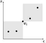
Passivity implies a certain structure on the state of the system, fully specified by the necessary and sufficient conditions given in Theorem 2. To summarise, a passive state is block-diagonal in the energy eigenbasis, with energies and eigenvalues that are ‘anti-ordered’. Our introduction of the - ensemble allows us to recast these conditions for passivity as a simple geometric property in . The key point here will be the idea of a total ordering on a vector space.
Definition 5.
Let and be two vectors in . Then we define the relation such that for any two vectors , we have if and only if and . Moreover, given a set of vectors, we say that is totally ordered if, given any two in , then either or .
With this definition in hand, we are now in a position to provide a simple characterisation of passive states in terms of the - ensemble.
Lemma 6.
A quantum state of a -dimensional quantum system satisfying is passive if and only if its associated - ensemble is a totally ordered set.
Proof.
This result follows directly from Theorem 2, since if and only if . ∎
As shown in Fig. (2), the total order appearing in Lemma 6 corresponds to a set of geometric constraints on the relative positioning of the elements of the - ensemble in . More precisely, if we pick out any element of the - ensemble, all other elements must lie within the upper-right or lower-left quadrant defined by the point .
3.3 -passivity and the - ensemble
Passivity is defined for a single system, while complete passivity shifts the focus onto multiple copies. Our introduction of the - ensemble lends itself well to this change of focus, precisely because it respects additivity under the composition of systems. Before outlining the key result, we first clarify this statement with a few examples.
It proves to be useful to ‘regularise’ the - ensemble by dividing by the number of copies of the system. For instance, given a qubit system () with - ensemble , the regularised representation for two copies of the state is
| (10) |
and for three copies it is
| (11) |
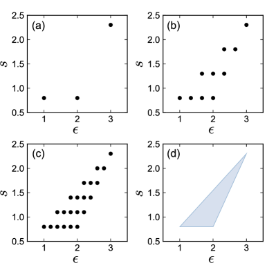
More generally, for some state of a -dimensional system with - ensemble , taking copies of the system gives
| (12) |
where . These are illustrated for a qutrit example in Fig. (3). The condition of -passivity for quantum states can now be geometrically restated.
Lemma 7.
A state of a -dimensional quantum system with Hamiltonian is -passive if and only if and is a totally ordered set.
Proof.
This is simply Lemma 6 stated for the - ensemble of copies of the state. ∎
Lemma 7 provides a natural algorithm for determining how many copies of a state are required before ergotropy arises, namely finding the lowest for which is not totally ordered. This offers greater simplicity than more algebraic approaches such as [13].
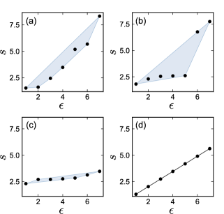
To consider complete passivity, we define an asymptotic version of the - ensemble, taking the limit of as , and making the intuition of Fig. (3) rigorous. The technical definition of this asymptotic ensemble is given in Appendix C, but here we need only consider a more intuitive picture, which views the IID asymptotic ensemble as the convex hull of the single-copy - ensemble.
Lemma 8 (Asymptotic ensemble).
For a -dimensional quantum system with Hamiltonian , and state with and - ensemble , we have that
| (13) |
where denotes the convex hull of a set .
The proof of this is provided in Appendix C. Some examples are pictured in Fig. (4). The significance of this is that in the asymptotic limit the structure of passive states is extremely simple – each passive state in the many-copy limit is described by a convex polygon in the plane that is easily obtained from the single-copy ensemble.
3.4 The geometric derivation of the Gibbs state
We now state the following elementary planar geometry result, which is needed for our Gibbs state derivation.
Lemma 9.
A convex set is totally ordered in if and only if all its points are colinear with a non-negative slope.
Proof.
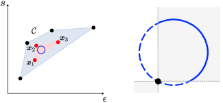
Consider a totally ordered convex set in , depicted in Fig. (5). Suppose there exist three points in that are not colinear. Convexity implies that the triangular region formed by their convex hull also lies in , and in particular any circle in this triangle is also in this set. However, it is impossible for a circle in the plane to be totally ordered, contradicting the initial assumption. The only way to avoid this contradiction is to enforce that all points of are colinear. Conversely, a convex set of colinear points in with non-negative slope is, by inspection, clearly totally ordered, which completes the proof. ∎
Theorem 10 (Complete passivity of Gibbs states).
A state of a -dimensional quantum system with Hamiltonian is completely passive if and only if it is a Gibbs state for some .
The proof is now obvious from the geometry of the situation.
Proof.
Suppose a state of a -dimensional system is completely passive. By definition, it is passive for all , thus must be totally ordered for all . This implies that must also be a totally ordered set. However, is convex, therefore Lemma 9 implies it must be a line segment with non-negative slope.
Since , each can be written as for some constants and . This implies that , thus is a Gibbs state at some inverse temperature .
Conversely, if is a Gibbs state with then it is clear that is a set of co-linear points with non-negative slope, and thus the convex hull is a totally ordered line segment with non-negative slope. The Gibbs state is therefore completely passive, which completes the proof. ∎
Note that this proof makes it immediately clear that all passive qubit states () are also completely passive, because the two points of their - ensemble have to be colinear. It is only for that there is a separation between passivity and complete passivity. We can re-state the condition for complete passivity in a purely geometric form.
Corollary 11.
A passive state of a -dimensional quantum system with Hamiltonian is completely passive / Gibbsian if and only if is totally ordered and the area of is zero.
This connects with the derivation in [9] that uses virtual temperatures which are defined as
| (14) |
and correspond to the gradient between the two points . The argument in [9] demonstrates that a negative virtual temperature is induced when enough copies of a state with multiple different virtual temperatures are considered, hence work can be extracted. This is equivalent to our statement that the - ensemble is no longer totally ordered, however there are some key differences in our new derivation. For instance, our derivation considers the state as a whole, rather than focusing on individual pairs of virtual temperatures. Moreover, our approach highlights the crucial role played by the boundaries of the - ensemble, while [9] does not make this distinction. This further motivates consideration of the asymptotic ensemble, where the convex hull of the - ensemble is taken. Finally we note that virtual temperatures are undefined for degenerate energy levels, while our approach incorporates these features in the same framework, as discussed in Appendix B.3. It is pleasing nonetheless that the structure of virtual temperatures naturally emerges in our framework.
In this geometric perspective, the points of the - ensemble for a completely passive state are colinear. The state has a single virtual temperature given by the gradient of this line, naturally interpreted as inverse temperature . While a completely passive state is fully specified by a single inverse temperature , other passive states are described by a set . This suggests a physical intuition as to why energy cannot be extracted from a completely passive state: if there are different virtual temperatures, a heat engine can be operated between them and work can be extracted [12].
Completely passive states of different systems at the same temperature will remain completely passive when combined. This can be immediately seen in our geometric description – points on the same line are closed under vector addition. This returns the usual thermodynamic temperature. However, the notion arising from complete passivity has the advantage that it applies to individual systems. Even an individual qubit in a completely passive state can be sensibly ascribed an inverse temperature .
4 Macroscopic non-equilibrium state variables.
The limit of many identical copies of a quantum state can be viewed as the macroscopic limit where we are interested in the physics of some large system in a state which is well described by a small list of intrinsic variables. Under such circumstances we can write , where is some -dimensional density matrix encoding the intrinsic variables and corresponds to the size of the total system. In traditional equilibrium thermodynamics the additive variables of internal energy and thermodynamic entropy are distinguished and form the basis of the resulting theory [29]. However, Sparaciari et al. [27] have recently shown that any two states and have the same values of and at the single copy level if and only if they are ‘asymptotically equivalent’ in the limit, irregardless of how far they are from equilbrium. Here asymptotic equivalence means that can be converted into as under energy conserving unitaries and involving an auxiliary system whose size is sublinear in . This result implies that macroscopic thermodynamic states specified by the two values of can be placed in a one-to-one correspondence with an equivalence class of microscopic variables , defined by the above notion of interconvertibility.
It is readily checked that for fixed values of there are multiple different compatible states , that have this average energy and entropy, for any fixed dimension . Each of these single-copy states will have a corresponding set of discrete points which has no area, being just a set of points. The macroscopic limit of many copies will be described by , which is a convex polyhedron in the plane with some area. It is important to emphasize that the convex shape does not describe a single copy of a state , but instead infinitely many copies of it. In other words is describing ‘’, which at the level of density matrices leads to highly problematic non-separable Hilbert spaces, however for passive states we have shown that an exact specification is provided by a simple geometric region in the 2-dimensional plane.
States in the same equivalence class , will have different asymptotic ensembles and these will in general have different areas in the plane. However from our earlier analysis, the unique geometric feature of equilibrium Gibbs states (and the emergence of a notion of temperature) is that the asymptotic ensemble becomes a line, with no area. This means that, despite the area of varying over an equivalence class of microscopic variables , for every macroscopic non-equilibrium state there must exist an ‘irreducible area’ variable that provides a quantification of how much the system deviates from equilibrium, under exactly the same levels of discrimination as occurring for macroscopic equilibrium thermodynamics. It is the aim of this section to study this ‘irreducible area’ and to connect it with existing measures of athermality. This prompts the following question:
Can we supplement the traditional macroscopic equilibrium variables with a sensible measure of the ‘irreducible area’ of that quantifies the degree to which the system deviates from equilibrium?
Two important points arise here. Firstly, because we are out of equilibrium such a variable is not considered relative to any one particular equilibrium state, but relative to the complete set of thermal equilibrium states. Secondly, we do not want to exploit the global structure of the manifold of equilibrium states in order to define this variable, but instead wish that it is defined purely from the statistics of the individual state under consideration. In the coming sections we provide an answer to the above question that satisfies these criteria. We first begin by setting up some basic notation.
4.1 Asymptotic equivalence and the energy-entropy diagram
Given a single-copy passive state we now interpret as a random variable that takes values in and which has expectation value
| (15) |
where is the average energy and is the von Neumann entropy of the state .
Asymptotic thermodynamics describes the limit where the number of non-interacting copies of the system tends to infinity. In this limit, we can define a notion of asymptotic equivalence between states as introduced by [27].
Definition 12.
Two -dimensional, -qudit states and with Hamiltonian are called asymptotically equivalent if there exists an ancilla system of many qudits whose Hamiltonian satisfies with state and unitary such that
| (16) |
where and denotes the trace norm.
Informally, we call two quantum states and asymptotically equivalent, and write , if we can transform between the two states via energy preserving unitaries in combination with some ancilliary system which is sublinear in size. The sublinearity of the ancilla size guarantees that, in the asymptotic limit, the amount of energy and entropy that can be transferred between the ancilla and each copy of the system tends to zero, meaning its per-copy contribution can be safely neglected. Asymptotic equivalence has been shown to pick out the two macroscopic variables identified in Eq. (15) as the two relevant quantities to describe the entire state space when the asymptotic limit is taken. This is expressed neatly in the following theorem, which was proven in [27].
Theorem 13.
Consider two arbitrary single-copy states and of a -dimensional quantum system with fixed Hamiltonian . Then the following equivalence holds
| (17) |
where denotes asymptotic equivalence in the many-copy limit.
Put simply, in the many-copy limit, any two states can be interconverted via unitaries that conserve energy globally if and only if they have the same average energy and entropy at the single-copy level. This allows us to define an equivalence class of states at the single-copy level for each pairing.
Definition 14 (Single-copy equivalence classes).
Given a quantum system with Hamiltonian , we define as the states of the system with average energy and entropy pair :
| (18) |
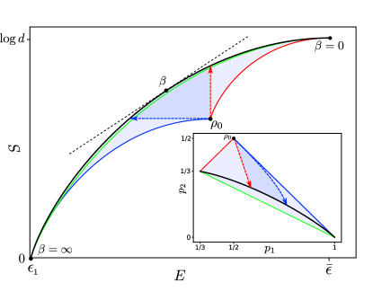
The union of all sets spans the entire space of states . Furthermore, the set of points corresponding to physical states form a closed convex subset in , known as the energy-entropy diagram [27]. It follows that under asymptotic equivalence, thermodynamics can be restricted to a -dimensional setting. Returning to our ensemble description, Eq. (15) shows that the statistical average or ‘centre of mass’ of all elements of a given ensemble corresponds to a single point on the energy-entropy (-) diagram.
The key features of the energy-entropy diagram are illustrated in Fig. (6) for a simple finite-dimensional system. The boundaries of the - diagram are fully determined by the particular Hamiltonian of the system . The space of states is bounded from above by the curve of Gibbs states with respect to , i.e., those which maximise the entropy for a given energy. Quantum states that are not completely passive lie below the equilibrium curve.
4.2 Area as a non-equilibrium variable
Asymptotic equivalence does not on its own describe a notion of thermal equilibrium. Therefore, as discussed, we want to supplement asymptotic equivalence with a notion of thermal equilibrium in a natural way. In the asymptotic many-copy limit, the ensemble is given by the convex hull of the single-copy ensemble , and has an associated area with being completely passive if and only if has zero area and non-negative slope. This area will in general vary over the equivalence class of single-copy states and therefore we must be careful in defining a measure that is well-defined on each equivalence class.
First, we need an explicit expression for the area variable. The area of is fully determined by the vertices of the convex hull, which by virtue of the relation between and are simply a subset of the points in .
Definition 15.
For a -dimensional quantum system in passive state , the set of vertices of the convex set is defined as
| (19) |
where denotes the set of extremal points of the convex set and the vertices are labelled clockwise modulo around the convex hull .
By the trapezium rule [30], the area of is then
| (20) |
where the sum runs over the elements of , and is the energy level spacing between the corresponding elements.
For a general -dimensional system, where , the area can vary as we range over all states in the equivalence class . However as discussed this area cannot decrease to zero since this would correspond to the state being an equilibrium state. We now define a canonical area for a given equivalence class , which we shall call the geometric athermality.
Definition 16.
Consider a -dimensional quantum system with fixed Hamiltonian . The geometric athermality for each pair is
| (21) |
where is the area of .
If the only information we have about a system is its average energy and entropy , the geometric athermality is a function of and but provides new information about the underlying state of the system. More precisely, it tells us whether or not the system is in thermal equilibrium with respect to any temperature. In other words, is a witness of athermality. This motivates the introduction of geometric athermality as our additional thermodynamic variable to supplement the asymptotic description , forming the triple of numbers .
In the remainder of this section, we show that this additional thermodynamic variable admits further operational interpretation by upgrading from a witness to a measure of athermality. More precisely, we show that is monotonically non-increasing under a set of physically motivated trajectories in the - plane that bring the state of the system closer to the manifold of Gibbs states.
We first clarify the set of physical trajectories in - space that concern us here. We restrict our attention to transformations of passive states that lead to work extraction and require that no ordered energy is injected into the system. Such transformations must therefore never increase the average energy or decrease the entropy of the system, since trajectories without these restrictions could involve the implicit smuggling-in of work resources. Hence, any infinitesimal evolution of the state is restricted in the direction of the shaded region in Fig. (6). Inspired by the activation maps introduced in [12], we call any state trajectory constructed from such infinitesimal transformations an activation trajectory, because it extracts ergotropy from the asymptotic collection of passive states , with .
Definition 17.
Any trajectory on the - diagram is called an activation trajectory if and only if its tangent unit vector satisfies and at all points along the trajectory directed towards the manifold of equilibrium states.
Activation trajectories can be constructed from isentropic and iso-energetic (at constant energy) thermalisations, represented by maps with appropriate thermal state . Physically, such maps can be realised by a partial thermalisation e.g. by bringing the system into thermal contact with a large heat bath at the appropriate temperature for a sufficient duration. For an iso-energetic trajectory, here is the thermal state with the same energy as the initial state . For an isentropic trajectory, is instead the thermal state with the same entropy as . This latter isentropic process is similar to an adiabatic process, and can be implemented via the protocol in [12] using sequential unitary interactions together with a large ‘weight’ system, such that any entropy changes that go to zero in the asymptotic limit.
Any small transformation in the - plane that is a convex combination of these two boundary cases will generate an activation trajectory. A sequence of such small transformations implements an arbitrary activation trajectory. We refer to [12] for more detail on the explicit construction of activation maps.
Equipped with the Definition 17, we now present the following theorem that justifies the use of as a sensible athermality measure.
Theorem 18 (Monotonicity of ).
For any -dimensional quantum system with non-degenerate Hamiltonian , the geometric athermality of a passive state is monotonically non-increasing along all activation trajectories.
A full proof is given in Appendix D, but for illustrative purposes, we sketch here the proof for a qutrit system. The extension to higher dimensions involves a protocol that generalises the simple qutrit case.
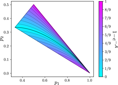
Consider a passive, but not completely passive, state of a qutrit system with non-degenerate Hamiltonian . For a qutrit system, there is a unique state333This follows from the fact that, for fixed we have three constraints on the spectrum of from conservation of average energy, entropy and normalisation and a 3-dimensional quantum system. Moreover, previous work has shown the - diagram is a closed convex subset of [27], and therefore . This implies that the mapping is bijective for qutrits (Fig. (6)). corresponding to each pair , i.e., . Therefore, the geometric athermality can be simply computed using Eq. (20) without performing the optimization in Definition 16. Due to the non-linearity of entropy, we do not have an analytic expression for in terms of and . However we can find a general, explicit expression for the differential of the geometric athermality for any passive qutrit state :
| (22) |
which is derived in Appendix D. The partial derivatives of this expression satisfy and , therefore the geometric athermality is monotonically decreasing along any activation trajectory, because the directional derivative at any point is
| (23) |
Since the geometric athermality is monotonically decreasing along activation trajectories for qutrits, we have shown it constitutes a non-trivial measure of athermality for such systems. The monotonicity for qutrit systems is also visually depicted in Fig. (7) over the entire passive region.
4.3 Relation of geometric athermality to –athermality, ergotropy and maximal heat extraction
The manifold of thermal equilibrium states is the boundary of quantum states as depicted in Fig. (6) and correspond to zero geometric athermality. However, is not the only measure of non-equilibrium behaviour that attains a zero value on the equilibrium curve. For example, completely passive states are the only states from which no work can be extracted in the IID limit, as well as the only states that can attain zero –athermality [27]. In this section, we consider how these quantities relate to the geometric athermality and, in particular, how the available work of a system in the asymptotic limit varies with .
The –athermality of a state measures the ‘distance’ on the - plane between the state and a specific Gibbs state at the point on the equilibrium curve. It is given by the relative entropy between the two states,
| (24) |
where is the free energy of state . This measure explicitly depends on the particular choice of Gibbs state . In particular, any Gibbs state with has non-zero –athermality. This measure is relevant for the usual resource-theoretic approach to thermodynamics, where systems can freely equilibrate with a thermal reservoir at inverse temperature [31]. However, in more general contexts, where all states on the equilibrium curve are considered equilibrium states, it is desirable to have a measure of athermality, like the geometric athermality, that does not have such a temperature dependence. In fact, Theorem 19 shows that the quantity is simply the entropy difference of state along the activation trajectory that thermalises it with zero work output. It can therefore be considered as a modified measure of athermality that no longer depends on temperature and attains a zero value for all Gibbs states.
We can therefore turn our attention to investigating the relation of the geometric athermality with the available work per system in the asymptotic limit. This is done by investigating certain simple activation trajectories on the - plane.
An isentropic trajectory that brings the state closer to the equilibrium curve is equivalent to work extraction with no entropic losses, so that the maximal extractable work of a state is
| (25) |
where is chosen so that the entropy remains constant along the trajectory, . This upper bound on the extractable work, which one could call the asymptotic ergotropy [26], has been shown to be attainable in [32] for the asymptotic regime of many identical copies of a state .
Correspondingly, an isoenergetic trajectory that brings the state on the equilibrium curve is equivalent to no work extraction. We can rephrase this thermodynamically as the activation trajectory that outputs the maximal entropic gain. It is given by an expression that is dual to Eq. (25) in the thermodynamic variables ,
| (26) |
where is now chosen so that the average energy remains constant, . This bound is attainable simply by thermalising the system at inverse-temperature . This bound can in fact be thought of as the minimal –athermality of state .
Theorem 19.
The maximal entropic gain for a system in a state along all possible activation trajectories is given by its minimal –athermality,
| (27) |
Proof.
By the defining relation Eq. (26) for and , we always have
| (28) |
To prove the second equality, we consider the the following two possible cases for any given state .
If , it coincides with and
| (29) |
If , we expand Eq. (24) to get
| (30) |
so that attains a unique extremum when . Since , this extremum is a minimum with value
| (31) |
∎
Geometrically, Theorem 19 says that the Gibbs state closest to with respect to the family of athermality functions is the one lying directly above on the - diagram.
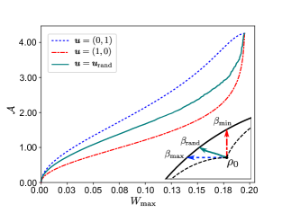
To illustrate the relation between the geometric athermality and asymptotic ergotropy (or minimal –athermality), we consider in Fig. (8) a maximally energetic passive qutrit state [11] under a Hamiltonian with equal energy spacing. The plot shows that the area of a 3-dimensional system and its asymptotic ergotropy are positively correlated along any activation trajectory. Similar results follow for the minimal –athermality.
In fact, we can show directly from their definitions that the two quantities are also measures of athermality. The differentials of asymptotic ergotropy and maximal entropic gain are
| (32) | ||||
| (33) |
where the temperatures are calculated at the point where the derivative is considered.
Theorem 20.
The asymptotic ergotropy and minimal –athermality are both monotonically non-decreasing functions of the geometric athermality along any differentiable activation trajectory.
Proof.
Let the activation trajectory be labelled , with non-positive slope along the entire trajectory due to Definition 17. Then, substituting in the differential forms of asymptotic ergotropy , minimal –athermality and geometric athermality , we find that, along the entire trajectory, the derivatives are positive. Therefore,
| (34) |
with equality whenever . ∎
The asymptotic ergotropy and minimimal –athermality are associated with the two extremal activation trajectories that a passive state can take towards the equilibrium curve. Therefore, one can calculate them by constructing the - diagram that corresponds to the - ensemble and then compute temperatures and respectively. The two measures are in a sense dual. On the contrary, the geometric athermality measure is not associated with any specific activation trajectory and solely depends on the - ensemble . This means that the geometric athermality does not require the whole structure of the - diagram and treats all points on the equilibrium curve equally, in the sense that there arises no special temperature like or .
A second point of comparison worth noting is the domain in which the three measures remain monotonic. The measures and are clearly monotonic at any point on the - plane that corresponds to a valid quantum state, while the monotonicity of the geometric athermality is guaranteed over the passive region of the - diagram. Although this reasoning seems to suggest that the geometric athermality is rather restricted, we can in fact easily extend its validity to all quantum states. Any state can be mapped to a unique passive state, associated to it via sorting its spectrum, while, conversely, one can reach any quantum state by unitarily transforming a passive state. Therefore, the entire - diagram can be divided into equivalence classes, each represented by a passive state , such that the value of the geometric athermality of a passive state can be associated to all quantum states in its equivalence class.
5 Outlook
In this paper, we have shed light on the structure of passive states and provided a clear and simple derivation of the Gibbs state. The key tool for this was a geometric reformulation of passivity as a total ordering. Equipped with the area of the - ensemble in this geometric framework, we then introduced the geometric athermality as a measure of athermality for quantum states that does not depend on a particular temperature. We also found that geometric athermality supplements the concept of asymptotic equivalence in a way that in a sense provides a non-equilibrium ‘equation of state’ . It might be fruitful to explore this line further to determine its scope and application.
We finish with a range of open questions that arise from the framework introduced in this paper:
-
1.
The main question that we have not explored is the following. For a –dimensional quantum system with Hamiltonian , and fixed values of what is the shape of the asymptotic ensemble that has minimal area? In other words, what is the general form of the quantum state whose asymptotic ensemble has area equal to the geometric athermality?
-
2.
It turns out that the accumulation of ‘face points’ (points in that lie on the boundary faces of ) appear to be significant (see the proof of the monotonicity of ). These lie on boundary line segments and so we can interpret each line segment as defining a Gibbs state at some inverse temperature . Can we describe the approach to equilibrium purely in terms of these boundary ‘equilibrium’ parameters?
-
3.
It would be of interest to provide a more unified geometric account of this structure and extend to other scenarios such as multiple non-commuting conserved charges (where will now consist of a volume in ).
-
4.
Can we extend the geometric description to include non-passive states, and states with coherences between energy eigenspaces?
-
5.
Can our geometric framework be extended to infinite-dimensional systems to enable the reformulation of the minimal area as a calculus of variations problem? What shape does the minimal surface assume in this continuum setting?
-
6.
We chose the Euclidean metric to define area. Is there a metric structure that provides a more natural form for the geometric athermality? Perhaps using ideas from information geometry?
6 Acknowledgements
We would like to thank Carlo Sparaciari for many useful discussions. NK, RA and TH are supported by the EPSRC Centre for Doctoral Training in Controlled Quantum Dynamics. TH is recently supported by EPSRC grant EP/T001011/1. DJ is supported by the Royal Society and also a University Academic Fellowship.
References
- Penrose [1969] O. Penrose, Foundations of statistical mechanics: a deductive treatment, International series of monographs in natural philosophy (Pergamon Press, 1969).
- Jaynes [1957a] E. T. Jaynes, Phys. Rev. 106, 620 (1957a).
- Jaynes [1957b] E. T. Jaynes, Phys. Rev. 108, 171 (1957b).
- Gogolin and Eisert [2016] C. Gogolin and J. Eisert, Rep. Prog. Phys 79, 056001 (2016).
- Cazalilla and Rigol [2010] M. A. Cazalilla and M. Rigol, New J. Phys. 12, 055006 (2010).
- Polkovnikov et al. [2011] A. Polkovnikov, K. Sengupta, A. Silva, and M. Vengalattore, Rev. Mod. Phys. 83, 863 (2011).
- Pusz and Woronowicz [1978] W. Pusz and S. L. Woronowicz, Comm. Math. Phys. 58, 273 (1978).
- Lenard [1978] A. Lenard, J. Stat. Phys 19, 575 (1978).
- Skrzypczyk et al. [2015] P. Skrzypczyk, R. Silva, and N. Brunner, Phys. Rev. E 91, 052133 (2015).
- Bratteli and Robinson [2003] O. Bratteli and D. Robinson, Operator Algebras and Quantum Statistical Mechanics: Equilibrium States. Models in Quantum Statistical Mechanics (Springer, 2003).
- Perarnau-Llobet et al. [2015] M. Perarnau-Llobet, K. V. Hovhannisyan, M. Huber, P. Skrzypczyk, J. Tura, and A. Acín, Phys. Rev. E 92, 042147 (2015).
- Sparaciari et al. [2017a] C. Sparaciari, D. Jennings, and J. Oppenheim, Nat. Commun 8 (2017a), 10.1038/s41467-017-01505-4.
- Salvia and Giovannetti [2020] R. Salvia and V. Giovannetti, Quantum 4, 274 (2020).
- Alhambra et al. [2019] A. M. Alhambra, G. Styliaris, N. A. Rodríguez-Briones, J. Sikora, and E. Martín-Martínez, Phys. Rev. Lett. 123, 190601 (2019).
- Alimuddin et al. [2020] M. Alimuddin, T. Guha, and P. Parashar, Phys. Rev. E 102, 022106 (2020).
- Balian and Balazs [1987] R. Balian and N. Balazs, Ann. Phys. 179, 97 (1987).
- Lostaglio et al. [2017] M. Lostaglio, D. Jennings, and T. Rudolph, New J. Phys. 19, 043008 (2017).
- Yunger Halpern et al. [2016] N. Yunger Halpern, P. Faist, J. Oppenheim, and A. Winter, Nat. Commun 7, 12051 (2016).
- Guryanova et al. [2016] Y. Guryanova, S. Popescu, A. J. Short, R. Silva, and P. Skrzypczyk, Nat. Commun 7, 12049 (2016).
- Boes et al. [2018] P. Boes, H. Wilming, J. Eisert, and R. Gallego, Nat. Commun 9, 1022 (2018).
- Bera et al. [2019] M. N. Bera, A. Riera, M. Lewenstein, Z. B. Khanian, and A. Winter, Quantum 3, 121 (2019).
- Uzdin and Rahav [2018] R. Uzdin and S. Rahav, Phys. Rev. X 8, 021064 (2018).
- Uzdin and Rahav [2019] R. Uzdin and S. Rahav, arXiv:1912.07922 (2019).
- Brown et al. [2016] E. G. Brown, N. Friis, and M. Huber, New J. Phys. 18, 113028 (2016).
- Binder et al. [2019] F. Binder, L. Correa, C. Gogolin, J. Anders, and G. Adesso, Thermodynamics in the Quantum Regime: Fundamental Aspects and New Directions, Fundamental Theories of Physics (Springer, 2019).
- Allahverdyan et al. [2004] A. E. Allahverdyan, R. Balian, and T. M. Nieuwenhuizen, EPL 67, 565 (2004).
- Sparaciari et al. [2017b] C. Sparaciari, J. Oppenheim, and T. Fritz, Phys. Rev. A 96, 052112 (2017b).
- Planck and Ogg [1945] M. Planck and A. Ogg, Treatise on Thermodynamics (Dover Publications, 1945).
- Callen [1985] H. Callen, Thermodynamics and an Introduction to Thermostatistics (Wiley, 1985).
- Riley et al. [1999] K. Riley, M. Hobson, and S. Bence, Am. J. Phys. 67 (1999), 10.2277/0521861535.
- Brandão et al. [2013] F. G. S. L. Brandão, M. Horodecki, J. Oppenheim, J. M. Renes, and R. W. Spekkens, Phys. Rev. Lett. 111, 250404 (2013).
- Alicki and Fannes [2013] R. Alicki and M. Fannes, Phys. Rev. E 87, 042123 (2013).
- Mirsky [1959] L. Mirsky, Math. Nachr. 20, 171 (1959).
- Hardy et al. [1988] G. H. Hardy, J. E. Littlewood, and G. Polya, Inequalities (Cambridge University Press, 1988).
- Marshall et al. [2011] A. W. Marshall, I. Olkin, and B. C. Arnold, Inequalities: Theory of Majorization and Its Applications (Springer, 2011).
- Perron [1907] O. Perron, Math. Ann. 64, 248 (1907).
- Markham et al. [2008] D. Markham, J. A. Miszczak, Z. Puchała, and K. Życzkowski, Phys. Rev. A 77, 042111 (2008).
- Schneider [2013] R. Schneider, Convex Bodies: The Brunn-Minkowski Theory, Encyclopedia of Mathematics and its Applications (Cambridge University Press, 2013).
- Tao and Vu [2006] T. Tao and V. H. Vu, Additive combinatorics., Vol. 105 (Cambridge University Press, 2006).
- Blizard [1988] W. D. Blizard, Notre Dame J. Formal Logic 30, 36 (1988).
- Haag et al. [1974] R. Haag, D. Kastler, and E. B. Trych-Pohlmeyer, Commun. Math. Phys 38, 173 (1974).
Appendix A Proof of Necessary and Sufficient Conditions for Passivity
Given a real vector , its components can be sorted into non-decreasing order, denoted by , or non-increasing order, denoted by . We say that another vector is majorized by , , if and only if for a bistochastic matrix . The theory of majorization leads to the following useful lemma.
Lemma 21.
For any two real finite-dimensional vectors and , and any bistochastic matrix , we have that
| (35) |
The first and last inequalities are a consequence of the lemma in [33], where we note that and that this majorization relation is invariant under permutation of vector components on either side, in particular permutations denoted by the arrows. The two middle inequalities together simply form a statement of the rearrangement inequality [34]. Informally this lemma says that given any two real-valued vectors, the maximum inner product over the ‘stochastic orbit’ of is obtained when the vector components of and are ‘aligned’ while the minimum inner product is obtained when they are ‘anti-aligned’. Moreover, bistochastic mixing of one of the vectors only moves the value of the inner product away from these two extremes. This structure is at the heart of passivity at the single-shot level, as we now explain.
Theorem 22.
Consider a -dimensional quantum system with Hamiltonian , with eigenvalue decomposition . A state of that system is passive if and only if and, for eigenvalue decomposition , we have that implies for all and in .
Proof.
Without loss of generality we label the energy spectrum so that and shift it appropriately so that all energies are non-negative. Then, the condition that implies for all and in is equivalent to .
We first demonstrate that a state satisfying with corresponding eigenvalues is passive. Firstly, is diagonalised in the energy basis, such that
| (36) |
with and average energy . The average energy of the transformed state is
| (37) |
where is a bistochastic matrix with elements . Lemma 21 implies that
| (38) |
for any unitary on the system, hence is passive.
Now we prove the other direction, beginning from the assumption that the state is passive. The density matrix for can generally be expressed in the energy basis as
| (39) |
which allows us to express the average energy as
| (40) |
By the Schur-Horn theorem [35], we have that , which is equivalent to for some bistochastic matrix . Lemma 21 then gives the minimum of this expression, . However, we assumed that is passive, hence equality holds, in particular
| (41) |
where bistochastic with the permutation matrix defined to send to .
Vectors and have non-negative entries and the energy spectrum is non-degenerate. Furthermore, the Perron-Frobenius theorem [36] bounds the eigenvalues of so that , hence the matrix has non-negative eigenvalues and is positive semi-definite. Therefore, the left hand side of Eq. (41) contains no negative terms and can only be zero for . The implication is that , so that is indeed diagonal in the energy eigenbasis with eigenvalues ‘anti-aligned’ with respect to . If degeneracies in energy exist we can coarse-grain the vectors and on these degenerate energy levels and reach the same conclusion, but now with no restriction on the ordering of the state eigenvalues within these degenerate eigenspaces. ∎
When considering passivity, it is assumed that we can perform any reversible (unitary) operations. The state space can therefore be partitioned into unitary orbits , which correspond to sets of mutually accessible states. Passive states are the energetic minima of the unitary orbits. Within each of these orbits, there must be at least one state that is passive.
We also note in passing that, by the same reasoning, the highest energy state in each unitary orbit (the most “impassive” state) has being diagonal in energy and with and now being ‘aligned’. The energy in this case is and thus the maximal work (ergotropy) that can be extracted from this state is given by . A more geometric discussion of these unitary orbits is provided in [37].
Appendix B Technical features of - ensembles
B.1 Additivity and the Minkowski Sum
Additivity enters our consideration when we compute the - ensemble of a combined system. Given states and with - ensembles and respectively, the state has - ensemble
| (42) |
where denotes usual vector addition in . The - ensembles combine according to the Minkowski sum [38] when we compose systems, which we write as
| (43) |
In the main text, we define the regularised - ensemble for copies of the state . The construction of is familiar in additive combinatorics, where it is more often termed the ’th sumset [39]. We leave for future work the question of whether results in additive combinatorics can be applied to the study passivity.
Composition of systems therefore has a well-studied mathematical structure that we can use in our analysis, including the useful fact that the Minkowski sum respects taking the convex hull:
| (44) |
B.2 Properties of the Asymptotic Ensemble
For a –dimensional system with Hamiltonian , we denote and . In terms of the generic features of asymptotic ensembles , we can make the following observations that are easily verified.
-
1.
We have that for all , and the closure of equals .
-
2.
For any passive state of a –dimensional quantum system, the asymptotic ensemble has a boundary given by a piece-wise linear concave function on for the upper boundary, and a piece-wise linear convex function on for the lower boundary.
-
3.
Any piece-wise linear concave or convex monotonically non-decreasing function on corresponds to a passive state of some quantum system with energy spectrum in . The (non-unique) eigenvalues of and are defined from the data for each being an end-point of a linear region for the function .
-
4.
Given monotonically non-decreasing piece-wise linear concave / convex functions, and respectively, the region contained by their intersection does not in general correspond to an asymptotic ensemble of some passive state. A simple counter-example is a square.
B.3 Degeneracy and Ground States
Degeneracy of the energy spectrum opens up the possibility of a group orbit having multiple passive states – simply permute the eigenvalues in the degenerate subspace. However, we consider unitary orbits as equivalence classes, therefore the energetic considerations depend only upon , and we choose a particular representative passive state (for example, take the eigenvalues for the degenerate subspace in non-increasing order).
Degeneracy introduces some subtleties to our geometric description of passivity, however the core derivation of the Gibbs state remains unchanged. A passive state is described by its - ensemble, but it is possible that degenerate levels correspond to the same pair . To handle this, we redefine the - ensemble as a multiset – a set in which elements can be repeated [40]. Geometrically, the repeated elements will occupy the same point in .
There are two main reasons for tracking such repeats in the - ensemble. Firstly, a passive state is representative of a whole unitary orbit , characterised by . The multiset representation records all eigenvalues regardless of repetition, and hence maintains complete information about the orbit . Minkowski addition can be defined for multisets practically unchanged, hence the composition of systems behaves exactly as before.
Secondly, this representation is able to adapt to perturbations that break the degeneracy of the energy spectrum. This relates to the notion of structural stability [41], the requirement that there is another state in the neighourhood of that is passive under a perturbed Hamiltonian in the neighbourhood of .
Structural stability follows from complete passivity unless the state is a ground state (where the only non-zero eigenvalues of reside in the lowest energy subspace). Complete passivity imposes that the eigenvalues of within a degenerate energy subspace must be equal (assuming is not a ground state). For suppose they were different, then would not be totally ordered, and hence no longer completely passive. This is handled straightforwardly in our geometric framework, as seen in Fig. (9).

The only caveat to this arises for ground states. All ground states are completely passive – it is clearly impossible to lower their energy. However, complete passivity does not imply structural stability for ground states. Complete passivity permits non-uniform eigenvalues in the ground subspace if no other energy subspaces are occupied, because the corresponding - ensemble remains totally ordered for arbitrary numbers of copies. However, should a small perturbation break the degeneracy of , there is no guarantee that a small perturbation to the ground state will make it once again completely passive.
Our physical framework should be robust to small perturbations, therefore structural stability is a desirable feature. This comes for free with the requirement of complete passivity, however it must be imposed additionally when considering ground states.
Appendix C Asymptotic passive state structure
Regularisation of the - ensemble converts points added by new copies of the system into convex combinations of the original elements of . We can re-express as
| (45) |
where . This set ranges over all probability distributions with rational components obtained from . As we increase , these probabilities tend towards non-negative real numbers.
Definition 23.
The asymptotic - ensemble of a system in the state , with Hamiltonian , is the set of limit-points of sequences , where . Specifically, given , there is a sequence , with that converges to under the standard vector norm on .
Lemma 24 (Asymptotic ensemble).
For a -dimensional quantum system with Hamiltonian , and state with and - ensemble , we have that
| (46) |
where denotes the convex hull of a set .
Proof.
As specified in the definition of , given an , then for any there exists a sequence of vectors for each , and an such that for all we have
| (47) |
Clearly for all . Moreover, since is finite dimensional, the set is a closed compact set in . The above inequality for all implies that and therefore .
Conversely, let , such that , where for all and . Construct the sequence of vectors with coefficients
| (48) |
where is the floor function defined by mapping a real number to the greatest integer that is not greater than this number. Then, and and therefore for all .
We now prove that the sequence converges to which implies that . Let be the decimal digit expansion of the -th coefficient of . Let and choose integer , where and . Then, for any we have,
| (49) |
The first equality follows from by definition of the floor function. The first inequality follows from the bound along with the decimal digit expansion of . The last inequality follows from . Therefore, every coefficient converges to , including , so the sequence converges to under the standard vector norm.
This argument holds for any choice of , so completing the proof. ∎
Appendix D Proof of geometric athermality monotonicity
The general structure of the proof is as follows. For systems of dimension , the geometric athermality is zero always and hence trivially non-increasing under activation trajectories. To prove the result for -dimensional quantum systems with , we proceed by considering a particular protocol for modifying the area by varying only 3 occupation probabilities in such a way that the ensemble area is monotonically non-increasing under infinitesimal isentropic and isoenergetic activation trajectories. We then utilise the defining property of the geometric athermality as the unique minimal area at each point on the - plane to make a general claim about how the geometric athermality varies under any activation trajectory. To this end, we begin by introducing the following primitive which we call a qutrit deformation.
D.1 Qutrit deformations
Definition 25.
(Qutrit deformation). Consider a -dimensional quantum system with and a passive, non-Gibbsian state of the system with non-degenerate Hamiltonian . We isolate a “virtual qutrit” by selecting three non-colinear elements . Then we can define a qutrit deformation to be some infinitesimal change to the area of , , generated by varying three occupation probabilities
| (50) |
of the virtual qutrit in isolation, in a region where all labels in Eq. (20) have a fixed correspondence to points.
Lemma 26.
Given and as in Definition 25, then we can always perform qutrit deformation to for all in the region of passive states such that we move non-trivially in the - plane under isentropic or isoenergetic processes.
Proof.
Consider a passive, but not completely passive, state of a -dimensional quantum system for with non-degenerate Hamiltonian . Let us label the three vertices of our virtual qutrit as for , and assume without loss of generality that . Let us further assume that the points in are not colinear (i.e. our virtual qutrit is not a ‘virtual Gibbs state’). So long as is not completely passive there are always at least three such non-colinear points to vary. Then, for an isentropic qutrit deformation, the two constraints given by conservation of probabilities and conservation of entropy reduce the differential of energy in terms of the variation of the single variable
| (51) |
Following a similar procedure for isoenergetic processes we obtain the following expression
| (52) |
where by our assumption that are not colinear and . Inspection of Eqs. (51) and (52) reveals that finite changes to the probabilities generate finite changes in energy and entropy, respectively, unless the three points for are colinear, which they are not by assumption. This completes the proof. ∎
Lemma 27.
Given and as in Definition 25, then the general expression for the differential of area under a qutrit deformation is given by
| (53) |
where the labels run modulo over points in , the labels run modulo clockwise around the set of vertices , and is the area associated with the virtual qutrit formed by the points in . Furthermore, we have defined the characteristic function such that
| (54) |
We note that is non-zero since is by definition assumed to be a set on non-colinear points.
Proof.
From Eq. (20) and the fact that for we obtain the following expression for the differential of the area under a qutrit deformation
| (55) |
Defining and , the system of three equations from the differentials of energy, entropy and normalisation can be written compactly as
| (56) |
The transformation matrix is invertible because the virtual qutrit is not completely passive by assumption, and so the columns of are linearly independent. Moreover, the determinant is related to the area of the qutrit ensemble via the simple relation
| (57) |
Therefore, we can invert Eq. (56), such that , for which we obtain
| (58) |
where etc. Direct substitution of Eq. (58) into Eq. (55) gives the result. ∎
D.2 Monotonically non-increasing deformations
Definition 28.
(Monotonically non-increasing deformation). Consider a -dimensional quantum system with and passive, full rank, non-Gibbsian state of the system with non-degenerate Hamiltonian . Then we define a monotonically non-increasing deformation to be some infinitesimal change to the area of , , generated by varying any number of occupation probabilities where , in such a way that we obtain
| (59) |
Then for or in Eq. (59) we have .
Definition 29.
(Upper branch). We define the upper branch such that
| (60) |
where the labels are ordered clockwise mod around .
We can then define the lower branch as follows.
Definition 30.
(Lower branch). We define the lower branch as the set difference
| (61) |
Definition 31.
(Face points). We define the set of face points associated with a given vertex point as
| (62) |
for any real-valued satisfying .
Lemma 32.
Let and be defined as in Definition 28. Then for any such initial state there exists at least one monotonically non-increasing deformation.
Proof.
Consider an initial passive, non-Gibbsian state of a -dimensional quantum system with and non-degenerate Hamiltonian . We show that via a careful selection of points we can always find a qutrit deformation of such that we obtain and , for infinitesimal transformations.
Inspection of Eq. (53) reveals that we obtain a monotonically non-increasing deformation if we choose our virtual qutrit such that for each . Since is passive, this reduces to the following set of energetic constraints:
| (63) |
To show that it is always possible to find such a set from any initial passive configuration, we can therefore project our ensemble onto the -axis and consider the relative signs of these energy differences. Importantly, since our Hamiltonian is assumed to be non-degenerate the mapping is a bijection.
We now state the protocol which is shown graphically in Fig. (10). We first consider the case where is not empty. The extremal points are always in the upper branch (white), so purely in terms of combinatorics there are four cases we need to consider, shown in Fig. (10)(a)-(d). By choosing the qutrit shown in each case, it is readily verified that the three equations Eq. (63) are satisfied. On the other hand, if is empty, by inspection the configuration shown in Fig. (10)(e) again satisfies conditions Eq. (63).
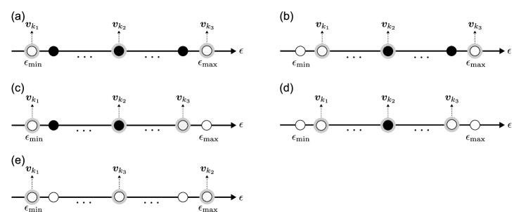
Complications can arise if there are face points associated with one or more of the vertices of our chosen virtual qutrit. Then our assumption that our function for computing area Eq. (20) is continuous over the domain on which the transformation takes place may break down. To combat this issue, in such cases, we can always appropriately replace the vertices of our virtual qutrit with face points or interior points in such a way that all labels in Eq. (20) have a fixed correspondence to points before and after the transformation. If all points get replaced with non-vertex points the qutrit deformation will yield from Eq. (53), which is indeed monotonically non-increasing.
For any initial passive state , the protocol described above returns a set of points that give rise to and under a qutrit deformation. Moreover, from Lemma 26 we have that this deformation allows for finite or . Therefore, we can always find a qutrit deformation that is a monotonically non-increasing deformation concluding the proof of Lemma 32.
∎
D.3 Proving monotonicity
We are now in a position to provide our proof of Theorem 18, which we restate for the purpose of clarity.
Theorem 33.
(Restatement). For any –dimensional quantum system with non-degenerate Hamiltonian , the geometric athermality of a passive state is monotonically non-increasing along all activation trajectories.
Proof.
In the following we restrict our attention to full rank states. This is desirable because the geometric athermality always remains finite and it is justified because points on the - diagram that contain full rank states form a connected dense subset of the passive region.
Consider an initial passive, full rank, non-Gibbsian state of a -dimensional quantum system with and non-degenerate Hamiltonian . For the area is zero for all and therefore is trivially non-increasing under activation trajectories. Now let and suppose that we pick the initial passive state with such an arrangement of populations that the ensemble area assumes the geometric athermality . We now consider an isentropic monotonically non-increasing deformation that takes us to some new state . From Lemma 32 such a deformation always exists, but is not guaranteed to take us to an area equal to the geometric athermality of the point . However, we can use the fact that under monotonically non-increasing deformations to show the following
| (64) |
where the second inequality follows from the definition of geometric athermality. Eq. (64) implies that an infinitesimal change in geometric athermality under any isentropic transformations is lower bounded by zero
| (65) |
and thus we have that . Now let us assume that we start again with an initial passive state corresponding to the geometric athermality and instead consider an isoenergetic monotonically non-increasing deformation that takes us to some new state . We can use the fact that under monotonic decreasing deformations to deduce the following
| (66) |
where the second inequality follows from the definition of geometric athermality. This implies that an infinitesimal change in geometric athermality under a constant internal energy transformation is upper bounded by zero
| (67) |
and so . Since the above argument applies to any passive non-Gibbsian initial state , we thus have that and , for all in the region of passive states ‘off the equilibrium curve’. In accordance with Eq. (23), we therefore find for that , whenever has components which satisfy and , in this region. Finally, as a consequence of Theorem 10, if the initial state is completely passive then the area assumes its global minimum value (zero). Since the thermal curve defines the set of states at the boundary of the state space, they can only be the end point of an activation trajectory. Therefore the geometric athermality is monotonically non-increasing over activation trajectories. ∎
