First simulation study of trackless events in the INO-ICAL detector to probe the sensitivity to atmospheric neutrino oscillation parameters

Abstract

The proposed India-based Neutrino Observatory will host a 50 kton magnetized iron calorimeter (ICAL) with resistive plate chambers as its active detector element. Its primary focus is to study charged-current interactions of atmospheric muon neutrinos via the reconstruction of muons in the detector. We present the first study of the energy and direction reconstruction of the final state lepton and hadrons produced in charged current interactions of atmospheric electron neutrinos at ICAL and the sensitivity of these events to neutrino oscillation parameters $\theta_{23}$ and $\Delta m_{32}^{2}$. However, the signatures of these events are similar to those from neutral-current interactions and charged-current muon neutrino events in which the muon track is not reconstructed. On including the entire set of events that do not produce a muon track, we find that reasonably good sensitivity to $\theta_{23}$ is obtained, with a relative $1\sigma$ precision of 15% on the mixing parameter $\sin^{2}\theta_{23}$, which decreases to 21%, when systematic uncertainties are considered.

I Introduction and Motivation

The phenomenon of neutrino oscillations arises when neutrino-mass eigenstates ($\nu_{1},\nu_{2}$ and $\nu_{3}$) coherently superpose to form neutrino-flavor states ($\nu_{e},\nu_{\mu}$ and $\nu_{\tau}$). The mass eigenstates and flavor states are related by a $3\times 3$ unitary matrix PMNS , which is parametrized by three mixing angles $(\theta_{12},\theta_{23}$ and $\theta_{13})$ and the $CP$-violating Dirac phase $\delta_{CP}$. Along with the dependence on these four parameters, the oscillation probability depends upon the mass-squared differences $\Delta m^{2}_{ij}\equiv m^{2}_{i}-m^{2}_{j}$, $(i\neq j)$, with $i$ and $j$ being any of the mass eigenstates. As only two of the three values of $\Delta m^{2}_{ij}$ are independent, oscillations are usually parametrized by $\Delta m^{2}_{21}$ and $\Delta m^{2}_{32}$. Hence, measurements of neutrino oscillations are only sensitive to the $\Delta m^{2}_{ij}$ and not to the neutrino masses.

Recent measurements from solar and reactor data Solar give the best-fit value of the “solar parameters” as, $\sin^{2}\theta_{12}=0.307^{+0.013}_{-0.012}$ and $\Delta m^{2}_{21}=(7.53\pm 0.18)\times 10^{-5}~{}\mathrm{eV}^{2}$ Solar_value . Furthermore, reactor $\bar{\nu}_{e}$ data precisely determines the mixing angle, $\theta_{13}$ Daya ; Chooz ; Reno . Measurements of atmospheric and accelerator neutrinos are sensitive to the “atmospheric parameters” $\Delta m_{32}^{2}$ and $\theta_{23}$. While $\left|\Delta m_{32}^{2}\right|=2.444\pm 0.034\times 10^{-3}~{}\mathrm{eV^{2}}$ newPDG has been measured, its sign, which determines the neutrino mass ordering, as well as the octant of $\theta_{23}$ are currently unknown. Current and near-future experiments Orca ; Pingu ; Dune can confirm the sign of $\Delta m^{2}_{32}$ being positive (normal ordering or hierarchy, NH) or negative (inverted ordering or hierarchy, IH), as well as resolve the octant problem i.e., $\theta_{23}=\pi/4$ (maximal mixing), $\theta_{23}<\pi/4$ (lower octant) or $\theta_{23}>\pi/4$ (upper octant). A global analysis of neutrino-oscillation parameters nufit favors the upper octant of $\theta_{23}$, with a best fit value of $\sin^{2}\theta_{23}=0.580^{+0.017}_{-0.021}$.

The proposed magnetized iron calorimeter (ICAL) detector at the India-based Neutrino Observatory (INO) is an experiment that can probe the mass hierarchy WP . The ICAL is most sensitive to atmospheric muon neutrinos (and anti-neutrinos), where the long tracks of muons produced in charged-current interactions of muon neutrinos (CC$\mu$) via $\nu_{\mu}N\to\mu^{-}X$ ($\overline{\nu}_{\mu}N\to\mu^{+}X$) can be used to reconstruct both the magnitude and direction of their momenta, as well as the charge of the muon. Here $X$ is any set of final-state hadrons. The advantage of having a magnetised iron calorimeter is its ability to clearly distinguish $\mu^{+}$ from $\mu^{-}$, which allows the differing matter effect for neutrinos and anti-neutrinos to be used to access the mass hierarchy. Hence analyzing muon events will yield the bulk of the sensitivity to oscillation parameters. Several studies of atmospheric neutrino oscillation parameters using muon events at INO have been reported Tarak ; Anushree ; Moonmoon ; Lakshmi .

Since neutrino experiments are statistically limited, any neutrino interactions that can be reconstructed in addition to the CC$\mu$ events in which there is muon track can potentially improve the sensitivity to oscillation parameters. Here we study the contribution from the sub-dominant electron-neutrino events, even though the detector configuration presents challenges in reconstructing the electron events correctly. In addition, CC$\mu$ events in which no track is reconstructed are considered, because they have an almost identical topology to the electron-neutrino interactions.

The ICAL will have sensitivity to atmospheric electron neutrinos (and anti-neutrinos) through the charged-current interaction (CC$e$), $\nu_{e}N\to eX$ ($\overline{\nu}_{e}N\to e^{+}X$). So only the final-state electromagnetic and hadronic showers can be used to reconstruct the event. The passive elements between each sampling layer in the ICAL are iron plates of 5.6 cm thickness, which corresponds to approximately three radiation lengths, so the detector will have limited capability to reconstruct the electromagnetic showers produced by the electrons. Previous simulation studies have characterized the sensitivity of ICAL to the hadron energy Lakshmi1 ; Moonmoon1 and preliminary results are available rawhit on its sensitivity to the hadron direction. Both the energy and direction are reconstructed through the pattern of hits that will be left by the hadronic shower in the detector. In this paper, for the first time, a detailed simulation study is made of the ability of the ICAL to reconstruct electrons and determine the $\nu_{e}$ momentum, and to examine the sensitivity of these events to neutrino-oscillation parameters. Such CC$e$ events appear as “trackless” events in the detector, in contrast to most CC$\mu$ events, where a final-state muon often produces a long track.

Note that there are other sources of trackless events, namely, neutral current (NC) events, where the final state lepton is not observed in the detector, as well as those CC$\mu$ events where the reconstruction algorithm for the muon track fails. In all these trackless events, only a shower is obtained; note, however, that for CC$e$/CC$\mu$ events, the shower includes hits from both electron/muon and the associated hadrons in the interaction while for NC events the shower is due to the hadrons alone. We analyze these trackless events and show that they have good sensitivity to the oscillation parameter $\theta_{23}$.

The rest of the paper is arranged in the following manner. We begin with the analysis of the pure CC$e$ sample in a hypothetical ICAL-like detector that is fully efficient and has perfect reconstruction of CC$e$ events. In Sec. 2 we identify the regions in electron-neutrino energy and direction space, where there is sensitivity to the oscillation parameters. In Sec. 3 we briefly describe the salient parts of the GEANT4 Geant41 ; Geant42 ICAL detector code that are used in the analysis, and also briefly discuss the generation of events in the detector using the NUANCE neutrino generator Nuance . In Sec. 4, we perform a $\chi^{2}$ analysis to determine the sensitivity of CC$e$ events to the neutrino-oscillation parameters, assuming a hypothetical ICAL-like detector. In Sec. 5, we consider the realistic case of sensitivity to oscillation parameters of the combined trackless sample of CC$e$, NC, and trackless CC$\mu$ events in the proposed ICAL detector at INO, including systematic uncertainties as well. We conclude with a discussion in Sec. 6.

II The oscillation probabilities

Detailed simulations studies indicating the potential of the ICAL to measure $\Delta m_{32}^{2}$ and $\theta_{23}$ have been performed using the dominant CC$\mu$ channel; these studies use reconstructed information about the muon momentum (magnitude and direction), the muon charge, and hadronic shower. Therefore, the contribution of CC$\mu$ events in determining the oscillation parameters is well-understood. Here we study the complementary set of events where no track could be reconstructed in the event sample. These events include CC$e$ events, which have hitherto not been studied with the ICAL.

Figure 1 shows the relevant oscillation probabilities for CC$e$ events, $P_{ee}$ and $P_{\mu e}$, as a function of the zenith angle $\theta_{\nu}$ (direction of the neutrino with respect to the vertically upward direction) for a single value of neutrino energy ($E_{\nu}=5$ GeV). Here $P_{ee}$ is the survival probability of $\nu_{e}$ and $P_{\mu e}$ is the probability of conversion of $\nu_{\mu}$ to $\nu_{e}$ Indu . In the top panel of Fig. 1, $P_{ee}$ and $P_{\mu e}$, are shown for three different values of $\Delta m_{32}^{2}$ while the bottom panel shows their behaviour for three different values of $\theta_{23}$. As can be seen from Fig. 1, the oscillation probability $P_{\mu e}$ is sensitive to both $\Delta m_{32}^{2}$ as well as $\theta_{23}$ while the survival probability $P_{ee}$ is sensitive to $\Delta m_{32}^{2}$ alone. In addition, the effect of the $\Delta m^{2}_{32}$ variation is opposite for both probabilities i.e., $P_{ee}$ increases with increasing $\Delta m^{2}_{32}$, $P_{\mu e}$ decreases with increasing $\Delta m^{2}_{32}$ and vice versa. The true values of the oscillation parameters used in this analysis is given in Table 1, along with the 3$\sigma$ confidence level (C.L.) for the parameters. We assume the normal ordering throughout this paper, unless otherwise stated, because trackless events have no sensitivity to mass-ordering as $\nu$ and $\bar{\nu}$ are indistinguishable.

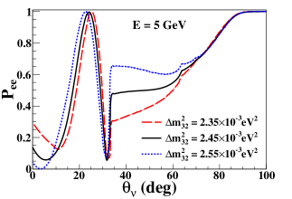
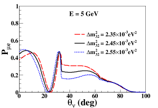
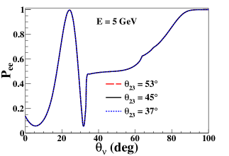
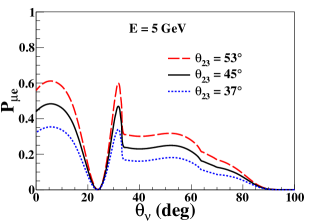
Figure 1: $P_{ee}$ (top left) and $P_{\mu e}$ (top right) as a function of zenith angle, shown for three values of $\Delta m^{2}_{32}$ ($2.55\times 10^{-3}~{}\mathrm{eV^{2}}$ [dotted blue line], $2.45\times 10^{-3}~{}\mathrm{eV^{2}}$ [solid black line], $2.35\times 10^{-3}~{}\mathrm{eV^{2}}$ [dashed red line]). $P_{ee}$ (bottom left) and $P_{\mu e}$ (bottom right) as a function of zenith angle, shown for three values of $\theta_{23}$ [left] ($53^{\circ}$ [dashed red line], $45^{\circ}$ [solid black line], $37^{\circ}$ [dotted blue line]).

Table 1: Oscillation parameter values assumed for the analysis PDG . The values of $\sin^{2}\theta_{12}$, $\sin^{2}\theta_{13}$ and $\Delta m^{2}_{12}$ have been fixed at their central value, because marginalizing them over their present 3$\sigma$ range causes very little change in the results.

Parameter	Value	3$\sigma$ range
$\sin^{2}\theta_{12}$	$0.307$	0.268 - 0.346
$\sin^{2}\theta_{23}$	$0.51$	0.39 - 0.63
$\sin^{2}\theta_{13}$	$0.0210$	0.0177 - 0.0243
$\Delta m^{2}_{21}~{}~{}[10^{-5}~{}\mathrm{eV}^{2}]$	$7.53$	6.99 - 8.07
$\Delta m^{2}_{32}~{}~{}[10^{-3}~{}\mathrm{eV}^{2}]$	$2.45$	2.3 - 2.6
$\delta_{CP}~{}~{}[\mathrm{deg}]$	0	0 - 360

To see a significant oscillation signature in the distributions of electron events, either the survival probability $P_{ee}$ should be significantly less than 1 or the appearance probability $P_{\mu e}$ should be significantly greater than 0. Therefore, we explore the parameter sensitivity in the regions where $P_{ee}<0.8$ and $P_{\mu e}>0.1$ as a function of $\cos{\theta_{\nu}}$ and $E_{\nu}$ to establish whether there is enough sensitivity to proceed with further studies. Fig. 2 shows $P_{ee}$ and $P_{\mu e}$ as a function of $E_{\nu}$ and $\cos\theta_{\nu}$. As expected both $P_{\mu e}$ and $P_{ee}$ show potential sensitivity in the region where $E_{\nu}>2$ GeV and $\cos\theta_{\nu}>0$, which corresponds to upward-going neutrinos, with the highest sensitivity in the region around $E_{\nu}\sim 5$ GeV and $\cos\theta_{\nu}\sim 0.7$.

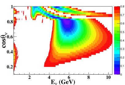
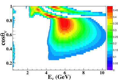
Figure 2: $P_{ee}<0.8$ (left) and $P_{\mu e}>0.1$ (right) as a function of $E_{\nu}$ and $\cos\theta_{\nu}$.

III Events Generation and Analysis

Atmospheric neutrinos originate from the decay of particles in hadronic showers generated by cosmic rays, which are primarily composed of protons, interacting with the upper atmosphere. The hadronic showers contain many charged pions that subsequently decay almost exclusively via the following chain:

$$\pi^{\pm}\rightarrow\mu^{\pm}+\nu_{\mu}(\overline{\nu}_{\mu});~{}~{}~{}~{}~{}\mu^{\pm}\rightarrow e^{\pm}+\nu_{e}(\overline{\nu}_{e})+\overline{\nu}_{\mu}(\nu_{\mu})~{}.$$

It can be seen that the flux of muon neutrinos ($\Phi_{\mu}$) is approximately twice the electron-neutrino flux ($\Phi_{e}$), especially at low energies where the muon subsequently decays before reaching the surface of the earth. These neutrinos interact with matter through CC and NC interactions.

III.1 Event generation with the NUANCE neutrino generator

Atmospheric neutrino interactions in the 50 kton ICAL detector for an exposure time of 100 years are simulated using the NUANCE neutrino generator, incorporating the Honda-3D atmospheric neutrino flux Honda . NUANCE generates these events for different cross sections, including quasi-elastic, resonance and deep-inelastic scattering. Since generating NUANCE events for various oscillation parameters is quite time consuming, it is generated once for a specified detector exposure time and the oscillation effects are later included event-by-event using the accept-or-reject method.

The number of events $N^{P}_{\alpha}~{}(\alpha=e,~{}\mu,~{}\tau)$ that occur via the processes $P$, $P=\mathrm{CC}$ or NC, in a detector with $N_{D}$ targets during an exposure time $T$, is related to the product of the flux times the cross section. Therefore,

$$N^{P}_{\alpha}=N_{D}\times T\int dE_{\nu}d\cos\theta_{\nu}\left[P_{e\alpha}\frac{d^{2}\Phi_{e}}{dE_{\nu}d\cos\theta_{\nu}}+P_{\mu\alpha}\frac{d^{2}\Phi_{\mu}}{dE_{\nu}d\cos\theta_{\nu}}\right]\,\sigma^{P}_{\alpha}(E_{\nu})~{},$$ (1)

where $\sigma^{P}_{\alpha}$ is the cross section for the interaction of neutrino flavour $\nu_{\alpha}$ via process $P$ in the detector. Here $\Phi_{e}$ and $\Phi_{\mu}$ are the electron and muon atmospheric neutrino fluxes respectively. A similar expression holds for anti-neutrinos as well.

In particular, $N^{\rm CC}_{e}$ and $N^{\rm CC}_{\mu}$ correspond to CC$e$ and CC$\mu$ interactions in ICAL. Note that

$$\sum_{\alpha}P_{\beta\alpha}=1~{},$$

for $\beta=e,\mu$, the sum of all NC interactions

$$N^{\rm NC}\equiv N^{\rm NC}_{e}+N^{\rm NC}_{\mu}+N^{\rm NC}_{\tau}~{},$$

is independent of oscillation probabilities, thus the oscillation parameters. Therefore, only $N^{\rm CC}_{e}$ and $N^{\rm CC}_{\mu}$ are sensitive to the neutrino-oscillation parameters.

III.2 Analysis of pure CC$e$ events

To understand the potential sensitivity to $\theta_{23}$ we start by performing a study assuming a hypothetical ICAL-like detector with 100% reconstruction efficiency and perfect resolution. This provides a benchmark for the maximum amount of information regarding neutrino oscillations that can be extracted from the ICAL data.

First a sample corresponding to five years of exposure that contains unoscillated $\nu_{e}$ and $\nu_{\mu}$ fluxes is considered. Then the following simulation algorithm is used to incorporate oscillations for CC$e$ events. The CC$e$ events have contributions from the $\nu_{e}$ fluxes via the first term in Eq. 1, viz., $\Phi_{e}\sigma_{e}^{CC}$, weighted by $P_{ee}$, and similarly from the $\nu_{\mu}$ flux via the second term. The weight is implemented as follows. A uniform random number $r$ between 0 and 1 is generated. Those events for which $P_{ee}>r$ are taken to be survived electron events. Similarly, NUANCE events are generated in which the electron and muon fluxes are swapped. This corresponds to events from the second term, viz., $\Phi_{\mu}\sigma^{CC}_{e}$, weighted by $P_{\mu e}$. Then the oscillation probability $P_{\mu e}$ is calculated for every swapped $\nu_{e}$ event; see Eq. 1. Those events for which $P_{\mu e}>r^{\prime}$, where $r^{\prime}$ is a uniform random number between 0 and 1, are taken to be oscillated electron events. Fig. 3 shows the fraction of CC$e$ events arising from survived and oscillated fluxes. Approximately 94% of $\nu_{e}$ events survive, while only $\sim 3\%$ of $\nu_{\mu}$ events oscillate into $\nu_{e}$ due to the smallness of $\theta_{13}$. However, note that these events are direction dependent; in addition, they arise from a term containing the atmospheric muon neutrino fluxes, as can be seen from Eq. 1, which are roughly twice the electron neutrino fluxes; hence the contribution of these events, roughly 6% of the total electron neutrino events, will turn out to be significant.

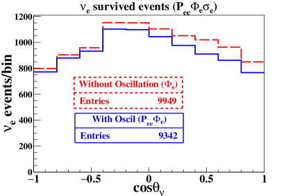
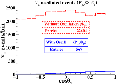
Figure 3: Simulated $\cos\theta$ distributions for CC$e$ events arising from survived $\nu_{e}$ (left) and oscillated $\nu_{\mu}$ events (right), with (solid blue line) and without (dashed red line) including oscillation probabilities $P_{\alpha e}$.

Figure 4 shows the ratio of oscillated to unoscillated events of the total (survived and oscillated) electron events. The oscillation signature is most prominent for up-going neutrinos ($\cos\theta>0.5$) with $E_{\nu}\sim 2$–7 GeV.

Similarly, five-year samples of CC$\mu$ events are generated using the same algorithm. The sensitivity of CC$\mu$ events to the oscillation parameters $\Delta m^{2}_{32}$ and $\theta_{23}$, via the dominant term proportional to $P_{\mu\mu}$, is well-understood and is not repeated here. Again, the “swapped events” in this case are also small due to the smallness of $P_{e\mu}$. Finally, five-year samples of NC events are generated in the same way and are independent of $P_{\beta\alpha}$.

The sensitivity and oscillation studies presented so far are for generator level events. For the studies that simulate the ICAL we need to reconstruct the events by a GEANT4-based detector simulation of the ICAL detector, and furthermore, select the trackless events in this sample.

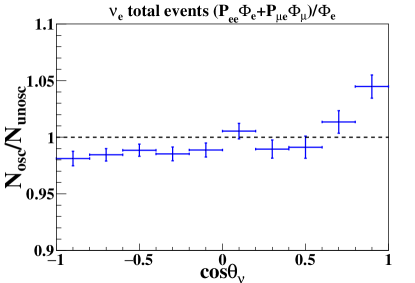
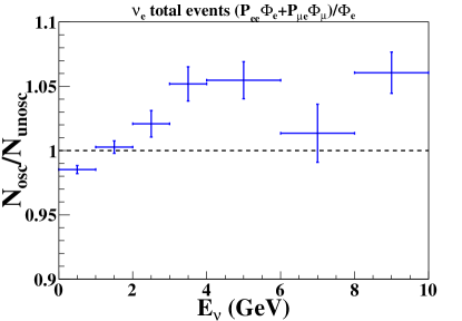
Figure 4: Ratio of oscillated to unoscillated CC$e$ events as a function of $\cos\theta_{\nu}$ (left) and $E_{\nu}$ (right), corresponding to five years of data.

III.3 Event generation with GEANT

A part of the INO proposal is the construction of a 50 kton magnetised ICAL Rajaji . The ICAL will be built in three modules each with a size of $16~{}{\rm m}\times 16~{}{\rm m}\times 14.5~{}{\rm m}$ (length $\times$ width $\times$ height). Each module will comprise of 151 layers of 5.6 cm thick iron plates, which will be magnetised to a strength of about 1.5 T using copper coils. The active detector elements of the ICAL will be the resistive plate chambers (RPCs) Rajaji . The RPCs are gaseous detectors constructed by placing 2 mm spacers between two 3mm thick glass plates of area $2~{}\mathrm{m}\times 2~{}\mathrm{m}$ and are operated at a high voltage of 10 kV in avalanche mode. Each of these RPCs will be interleaved into the 4 cm gap between the iron layers. The detector will be sensitive to muons and other charged particles produced in the interactions of atmospheric neutrinos with the iron nuclei. This geometry and magnetic field have been coded into a GEANT4-based simulation of the detector response. The RPCs are considered to have a timing resolution of 1 ns, which is important to distinguish up-going from down-going events.

The dominant signals from atmospheric neutrinos in the ICAL detector are from CC$\mu$ events. The CC$e$ events form the sub-dominant signal, both due to smaller fluxes and also because ICAL is optimised for detecting CC$\mu$ events. We also have NC interactions, but the cross section for these interactions are small compared to CC$\mu$ interactions crossec .

The NUANCE-generated events are passed through the GEANT4-based simulation of the ICAL detector. Each event leaves a pattern of hits in the sensitive RPC detector. Long track-like events are typically associated with the minimum-ionising muons. Using information about the local magnetic field that is incorporated into the GEANT code, a Kalman-filter algorithm Kalman is used to identify and reconstruct possible “tracks” which can be fitted to yield the particle momentum and sign of charge. Events where no track could be reconstructed are identified as trackless events. Notice that events which pass through less than four layers of the detector are not sent to the Kalman filter for track reconstruction and hence are included in the trackless events sample. The composition of this sample is shown in Fig. 5. While roughly half the events in the vertical bins are from CC$e$ events, the bins in the horizontal direction are dominated by trackless CC$\mu$ events. (About 1% of the time, an energetic pion from a hadron shower may give a track and the event may be misidentified as a CC$\mu$ event.) In order to analyze these events we need to calibrate the hits to the energy and direction associated with each event. We first consider the CC$e$ events alone.

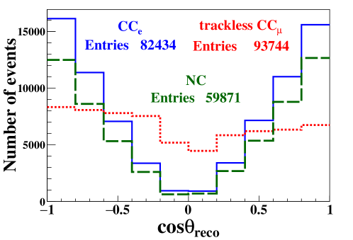
Figure 5: $\cos\theta_{\rm reco}$ distribution for five-year samples of CC$e$ (blue solid line), trackless CC$\mu$ (red dotted line) and NC (green dashed line) events.

III.4 Direction reconstruction of trackless events

To reconstruct the direction of the shower, we use a method referred to as the raw-hit method rawhit . A charged particle, produced by the interaction of neutrinos with the detector, while passing through an RPC, produces induced electrical signals. These signals are collected by copper pick-up strips of width 2 cm, which are placed orthogonal to each other on either side of the RPC. The center of the pick-up strips defines $x$ or $y$ coordinate of the hits and the center of the RPC air-gap defines the $z$ coordinate. The signals in the copper strips thus provide either $(x,z)$ or $(y,z)$ information and are considered as “hits”, which are used to reconstruct the average energy and direction of the shower. Due to the coarse position resolution of the ICAL detector, it is difficult to distinguish between electron and hadron showers. Since in CC$e$ and CC$\mu$ trackless events the shower actually arises from both the electron/muon and hadrons in the final state, the net reconstructed direction will point back to that of the original neutrino, especially at higher energies since the final state particles from such events are forward-peaked. This is in contrast to the direction reconstruction of showers in CC$\mu$ events where the muon track is reconstructed; here, the direction of the shower determines the net direction of the hadrons alone, since the direction of the muons can be independently determined. Finally, since the final state lepton is not detected in NC events, the shower direction is that of the hadrons in the event, just as in the case of CC$\mu$ events with track reconstruction.

If two or more $x$ and $y$ strips have signals within a single RPC in an event, there is an ambiguity in the definition of the $(x,y)$ hit position. One or more of the positions are fake and are referred to as a ghost hit. Therefore, the reconstruction is done separately in the $x$-$z$ and $y$-$z$ planes to avoid these ghost hits. Since the electron or hadron showers are insensitive to the magnetic field, the average direction of the shower is reconstructed as,

$$\theta_{\rm reco}=\mathrm{tan}^{-1}\sqrt{m_{x}^{2}+m_{y}^{2}};~{}~{}~{}~{}~{}\phi=\mathrm{tan}^{-1}\left(\frac{m_{y}}{m_{x}}\right)~{},$$ (2)

where $m_{x[y]}$ are the slopes of straight line fits to the $(x,z)$ [$(y,z)$] hit positions. The simulation requires that the hits are within a timing window of 50 ns to ensure they are only from the event under consideration. Requirements on the minimum number of layers with hits ($\geq 2$) and minimum number of hits per event $n_{\rm hits}$ ($\geq 3$) are applied at the reconstruction level to ensure that there are sufficient hits passing through enough layers to fit a straight line. Around 46% of the events satisfy these criteria. The time information from each of these hit distributions i.e., the slopes of the $t_{x}$ vs. $z$ and $t_{y}$ vs. $z$ distributions, allows us to reconstruct whether the event is an up-going or down-going one. Approximately 10% of events have time slopes from the $t_{x}$-$z$ and $t_{y}$-$z$ distributions of opposite signs; these events are discarded. Figure 6 shows an example of an up-going event and the corresponding position of hits in that event in the $x$-$z$ and $y$-$z$ planes.

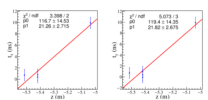
Figure 6: Example fits (top panel) to $z$ vs. $t_{x}$ (left) and $z$ vs. $t_{y}$ (right) distributions for one event which was produced by an electron neutrino with $E_{\nu}$ = 1.59 GeV and $\cos{\theta_{\nu}}$ = 0.48. Fits to the distribution (bottom panel) of $z$-$x$ (left) and $z$-$y$ (right) hits for the same example event. Here $p0$ and $p1$ are the intercept and slope of the fit, respectively.

The reconstruction efficiency $\epsilon_{\rm reco}$ and relative directional efficiency $\epsilon_{\rm dir}$ are given by,

$$\epsilon_{\rm reco}=\frac{N_{\rm reco}}{N}~{},\hskip 56.9055pt\epsilon_{\rm dir}=\frac{N^{\prime}_{\rm reco}}{N_{\rm reco}}~{},$$ (3)

where $N_{\rm reco}$ is the number of events reconstructed from the total number of events ($N$) and $N^{\prime}_{\rm reco}$ is number of the events correctly reconstructed as up-going or down-going. Figure 7 shows $\epsilon_{\rm reco}$ and $\epsilon_{\rm dir}$ as functions of $\cos\theta_{\nu}$. The $E_{\nu}$ and $\cos\theta_{\nu}$ averaged values of $\epsilon_{\rm reco}$ and $\epsilon_{\rm dir}$ are $(41.7\pm 0.2)\%$ and $(66.8\pm 0.2)\%$, respectively, showing that we can distinguish the up-going event from the down-going event, which is crucial for the oscillation studies.

Figure 8 shows the $\cos\theta_{\nu}$ distribution before and after reconstruction. Notice that angular smearing leads to an excess of events in the vertical directions compared to the NUANCE level events while leaving very few events in the horizontal bins.

Figure 7: Reconstruction efficiency, $\epsilon_{\rm reco}$ (left) and the relative directional efficiency $\epsilon_{\rm dir}$ (right) as a function of $\cos\theta_{\nu}$. Note that the $y$-axis scales on the two graphs are different.

Figure 8: The distribution of the $\cos\theta_{\nu}$ (dashed red line) and reconstructed $\cos\theta_{\rm reco}$ (solid blue line).

III.5 Energy reconstruction of trackless events

The total energy reconstructed from the hit information is labelled as $E_{\rm reco}$. As discussed above, for the CC$e$ and CC$\mu$ events sample, this should give the incident neutrino energy while for NC events, this is the hadron energy in the final state. It is not possible to obtain the reconstructed energy directly from the hit information; rather it is inferred via a calibration of the number of hits as a function of the true energy. Taking into consideration the same selection criteria applied for direction reconstruction, we remove three hits from each event so that we calibrate true energy vs. $(n_{\rm hits}-3)$. Distributions of hits in distinct energy ranges are formed. (Figure 9 (left) shows an example of hits distribution in the energy range 5.9 to 6.4 GeV for CC$e$ events). For each of these hit distributions, the mean of number hits $\overline{n}(E)$ is plotted against the mean energy $\overline{E}$ of events within a specific energy range. This data is then fit to,

$$\bar{n}(E)=n_{0}-n_{1}\exp(-\bar{E}/E_{0})~{},$$ (4)

where $n_{0}$, $n_{1}$ and $E_{0}$ are constants, as shown in the right side of Fig. 9.

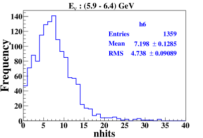
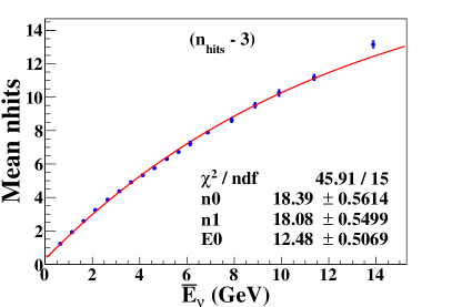
Figure 9: Left: example of hits distribution in the $E_{\nu}$ range (5.9 to 6.4) GeV. Right: $\overline{n}(E)$ vs. $\overline{E}$ with the fit superimposed.

After obtaining the values of constants $n_{0}$, $n_{1}$ and $E_{0}$, we invert Eq. 4 to estimate the reconstructed energy, $E_{\rm reco}$. In Fig. 10, which shows the $E_{\nu}$ distribution before and after reconstruction, we see that the reconstructed events have shifted towards high energy. Most of the low energy events are reconstructed as high energy events because of the upper tail in $n_{\rm hits}$ distribution (see Fig. 9), because of which we have more reconstructed events with higher energy.

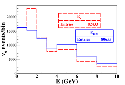
Figure 10: Distribution of true $E_{\nu}$ (dashed red lines) and reconstructed $E_{\rm reco}$ (solid blue lines) energy for CC$e$ events.

III.6 Sensitivity after reconstruction

Using the simulation algorithm the oscillations were again incorporated in the unoscillated flux of reconstructed $\theta_{\rm reco}$ and $E_{\rm reco}$. Figure  11 shows the ratio of oscillated to unoscillated $\cos\theta_{\rm reco}$ and $E_{\rm reco}$ distributions for selected events. As seen in Fig. 4, where we had taken a sample corresponding to five-year data assuming 100% efficiency and perfect resolution, even after reconstruction the oscillation signature is still prominent in regions where $E_{\nu}>2$ GeV and $\cos\theta_{\nu}>0.5$.

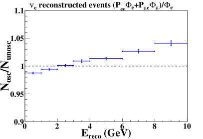
Figure 11: Ratio of oscillated to un-oscillated CC$e$ events as a function of $\cos\theta_{\rm reco}$ (left) and $E_{\rm reco}$ (right), for 50$\times$100 kton-years of exposure time.

IV Sensitivity of electron events to oscillation parameters

To assess the sensitivity of pure CC$e$ events in ICAL to oscillation parameters, a $\chi^{2}$ analysis is performed assuming an ICAL-like detector that can also perfectly reconstruct and discriminate such pure CC$e$ events; the analysis including all trackless events is presented in the next section. First, a set of 100 years of data is simulated with the true values of the oscillation parameters as given in Table 1, which is later scaled down to 10 years for the statistical analysis. The simulated data are then fit to the theoretical expectation for a set of oscillation parameters varied in their $3\sigma$ ranges, by binning it in ten $\cos\theta_{\rm reco}$ bins of equal width and seven $E_{\rm reco}$ bins of unequal width in the range 0 to 10 GeV (see Fig. 11). The fit is the minimization of a Poissonian $\chi^{2}$

$$\chi^{2}=2\sum_{i}\sum_{j}\Bigg{[}(T_{ij}-D_{ij})-D_{ij}\ln\bigg{(}\frac{T_{ij}}{D_{ij}}\bigg{)}\Bigg{]}~{},$$ (5)

where $T_{ij}$ and $D_{ij}$ are the “theoretically expected” and “observed number” of events respectively, in the $i^{\mathrm{th}}$ $\cos\theta_{\rm reco}$ bin and $j^{\mathrm{th}}$ $E_{\rm reco}$ bin. We find that this hypothetical case with a sample of just CC $\nu_{e}$ events, without including other trackless events and systematic uncertainties, does show sensitivity to neutrino oscillation parameters.

Figure 12 shows the effect of binning in $\cos\theta_{\rm reco}$ and $E_{\rm reco}$ separately, as well as binning in both observables. With binning in $\cos\theta_{\rm reco}$ alone, we find that it is possible to obtain a relative $1\sigma$ precision on $\sin^{2}\theta_{23}$ of 20%. There is no significant change when the events are binned in both observables. Therefore, for the rest of the analysis we present results from fits to $\cos\theta_{\rm reco}$ bins alone, with events summed over all $E_{\nu}$. Since the effect of increasing (decreasing) $\Delta m_{32}^{2}$ leads to an increase (decrease) and decrease (increase) in $P_{ee}$ and $P_{\mu e}$, respectively (Fig. 1 top panel), sensitivity to $\Delta m^{2}_{32}$ from CC$e$ events in ICAL is inconsequential. Hence in the rest of the paper we consider the sensitivity to $\theta_{23}$ alone. We now consider a realistic analysis of all trackless events.

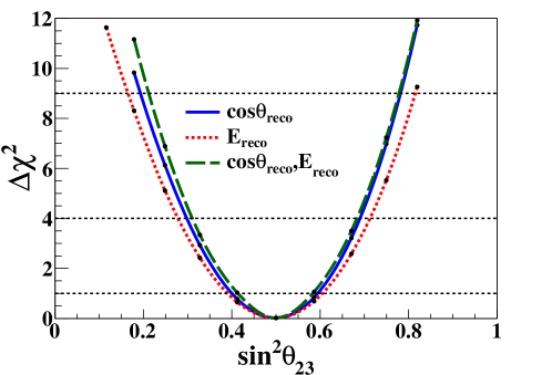
Figure 12: $\Delta\chi^{2}$ as a function of $\sin^{2}\theta_{23}$ with bins in $\cos\theta_{\rm reco}$ (solid blue lines) alone, $E_{\rm reco}$ (dotted red lines) alone and in both (dashed green lines) $\cos\theta_{\rm reco}$ and $E_{\rm reco}$. “Data” were generated with true $\sin^{2}\theta_{23}=0.5$.

V Realistic analysis of trackless events in ICAL

V.1 Selection criteria

Since the CC$e$ events have been reconstructed through their showers (both electromagnetic and hadronic), the NC events that produce showers (only hadronic) may be misidentified as CC$e$ events, even though we expect the shower pattern to be different in these two cases. A useful set of parameters to separate these events is the number of layers ($l$) that the shower has traversed and the average hits per layer $(s/l)$ in an event, $s$ being the number of hits in that layer LSMthesis . While both CC$e$ and NC events are expected to traverse fewer layers than CC$\mu$ events (since the muon is a minimum-ionising particle that leaves long “tracks” in the detector), it is expected that CC$e$ events will have larger $s/l$ because of the nature of the events. In addition, sometimes, due to large scattering or low energies giving a small number of hits, the Kalman-filter algorithm fails to reconstruct even a single track for CC$\mu$ events. Hence such “trackless” events also have showers as their signatures in the detector and can also be misidentified as CC$e$ or NC events. In a realistic analysis with a detector such as ICAL, all these events need to be considered together. It turns out that this fraction is substantial; about 53% of the total CC$\mu$ events, which occurs because of the large fluxes at low energies. Such events have very small $s/l\sim 1.5$ due to the minimum-ionising nature of muons, as can be seen in Fig. 13. It can be seen that requiring $s/l>2$ increases the purity of CC$e$ events, but it decreases the number of events in the sample, especially since a large fraction of CC$e$ events correspond to low energies and hence traverse fewer layers. Here, efficiency is defined as the percentage of CC$e$ events passing the $s/l$ selection in total CC$e$ events and purity is the percentage of CC$e$ events in all type of events passing $s/l$ selection.

Figure 13: Mean of average hits per layer($s/l$) as a function of number of layers($l$) for CC$e$ (blue triangle), trackless CC$\mu$ (red star) and NC (pink circle for NC$e$ and green square for NC$\mu$) events.

Different selection criteria on $s/l$, $s/l>1$, $s/l>1.4$, $s/l>1.8$, and $s/l>2$, were used and the sensitivity to $\sin^{2}\theta_{23}$ determined. It was found that the sensitivity is dominated by the statistics, since the harder cuts decrease the total number of events available in the analysis. While efforts are on going to improve the Kalman-filter algorithm, as well as to improve the efficiency of separating the CC$e$ from the NC and trackless CC$\mu$ events, in what follows, we include all events (CC$e$, NC and trackless CC$\mu$) in the analysis and do not apply any further selection criteria on $s/l$.

In the next section of this paper, we examine the effect of the inclusion of all these trackless events on the sensitivities to the neutrino-oscillation parameters.

V.2 $\chi^{2}$ analysis of the entire sample of trackless events

We now repeat the $\chi^{2}$ analysis, including all trackless events. As before, the parameters not being studied are fixed at their true values as given in Table 1. Since $\theta_{13}$ is so precisely known, it is also kept fixed in the analysis. We consider the inclusion of systematic errors in the next section.

With the inclusion of all trackless events, the Poissonian $\chi^{2}$ without systematics is:

$$\chi^{2}=2\sum_{i}\left[T_{i}-D_{i}-D_{i}\ln\left(\frac{T_{i}}{D_{i}}\right)\right]~{},$$ (6)

where $T_{i}$ now include the original CC$e$ events, and both the NC and trackless CC$\mu$ events as well, in the $i^{\mathrm{th}}$ $\cos\theta_{\rm reco}$ bin. The result of the analysis for the sensitivity to $\sin^{2}\theta_{23}$ is shown in Fig. 14. It can be seen that inclusion of all trackless events increases the relative 1$\sigma$ precision on $\sin^{2}\theta_{23}$ to 15%. The improvement in sensitivity to $\sin^{2}\theta_{23}$ can be understood as the effect of inclusion of the low energy trackless CC$\mu$ events ($\sim$ 42% of total CC$\mu$ events), since NC events do not have sensitivity to oscillation parameters and simply improve the overall normalization uncertainties.

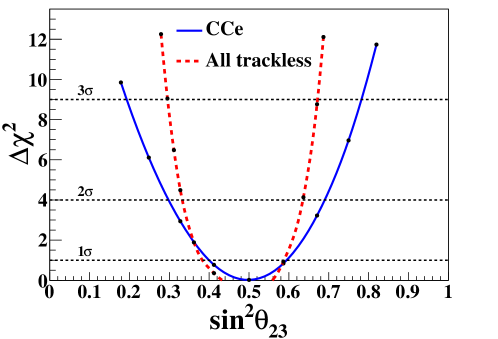
Figure 14: $\Delta\chi^{2}$ as a function of $\sin^{2}\theta_{23}$ with only CC$e$ events (solid blue lines) compared with the sensitivity when all trackless events (dotted red lines) are included.

V.3 Including systematic uncertainties

So far, we have not considered the effect of systematic uncertainties on the sensitivities. We incorporate them through the pull method pull1 ; pull2 , where each independent source of systematic uncertainty is added to the difference of the theoretically expected and observed events through an univariate gaussian random variable ($\xi$) referred to as the pull. To avoid overestimation of the systematic uncertainties, penalties are implemented by adding $\xi^{2}$ terms. We consider two sources of systematic uncertainties: $(i)$ a 5$\%$ uncertainty on the flux dependency on $\theta_{\nu}$ pull1 and $(ii)$ a 2$\%$ uncertainty on the efficiency of reconstruction. In principle, it is possible to include an additional systematic uncertainty due to the overall flux normalisation; however, a detailed analysis of the higher energy ($E_{\nu}>1$ GeV) CC$\mu$ events Rebin has shown that such a detector can determine the overall normalisation to about 1.5% and hence we ignore this source of uncertainty.

V.3.1 Uncertainties due to reconstruction

The uncertainty on the efficiency of reconstruction of the evernt is uncorrelated between CC$e$, CC$\mu$ and $NC$ events. This is because the contribution from CC$\mu$ events includes mainly the low energy events (which do not have sufficient hits to be reconstructed in the Kalman filter) while the entire CC$e$ sample corresponds to low energies since the electron-neutrino fluxes are much softer than the muon-neutrino fluxes (the latter arises only in the secondary three-body decay of the cosmic muons). On the other hand, the reconstruction efficiency for NC events is small because they do not survive the minimum number of hits ($\geq 3$) criterion required to reconstruct their direction, which is the result of the final-state neutrino taking away a substantial part of the available energy. While CC$e$ events also arise from a softer flux spectrum, the presence of electrons in the final state adds to the total number of hits and hence more CC$e$ events pass these selection criterion. In any case, it can be seen that the reconstruction efficiencies of the different events contributing to the analysis have different origins and are hence uncorrelated. We therefore apply a 2% systematic uncertainty on the reconstruction efficiencies, but include them in the analysis as three different uncorrelated pulls, one for each channel.

With the addition of these systematics, the $\chi^{2}$ now becomes,

$$\chi^{2}=\min_{\{\xi\}}\sum_{i}2\left\{N_{i}(\xi)-D_{i}-D_{i}\ln\left[\frac{N_{i}(\xi)}{D_{i}}\right]\right\}+\xi_{Z}^{2}+\xi_{\mathrm{CC}e}^{2}+\xi_{CC_{\mu}}^{2}+\xi_{NC}^{2}~{},$$ (7)

where the total events are given in terms of the CC$e$ ($T_{i}^{\mathrm{CC}e}$), CC$\mu$ ($T_{i}^{\mathrm{CC}\mu}$) and NC ($T_{i}^{\rm NC}$) events as,

$$N_{i}(\xi)\equiv\left\{\left(T_{i}^{\mathrm{CC}e}+T_{i}^{\mathrm{CC}\mu}+T_{i}^{\rm NC}\right)\,\left(1+\pi_{i}\xi_{Z}\right)+\pi_{i}^{\rm reco}\left(T_{i}^{\mathrm{CC}e}\xi_{\mathrm{CC}e}+T_{i}^{\mathrm{CC}\mu}\xi_{\mathrm{CC}\mu}+T_{i}^{\rm NC}\xi_{\rm NC}\right)\right\}~{},$$ (8)

where $\pi_{i}$ is the correlated systematic uncertainty in the zenith-angle dependence for the different sets of events, and $\xi_{Z}$ is the corresponding pull. Although the same uncorrelated error $\pi_{i}^{\rm reco}$ is applied across all sets of events, three different pulls are applied to the CC$e$ ($\xi_{T}$), trackless CC$\mu$ component ($\xi_{CC{\mu}}$) and NC component ($\xi_{NC}$) respectively, to account for the varying signatures of these events.

The analysis is repeated with the inclusion of uncertainties on all three types of trackless events. As expected, the sensitivity decreases, as can be seen in Fig. 15, which shows $\Delta\chi^{2}$ as a function of $\sin^{2}\theta_{23}$ with and without pulls. The results are also then marginalized over the $3\sigma$ range of the remaining neutrino oscillation parameters (excluding the solar parameters), as given in Table 1 and the result plotted in Fig. 15. The inclusion of systematic uncertainties as well as marginalisation, reduces the relative 1$\sigma$ precision on $\sin^{2}\theta_{23}$ from 15% to 21%.

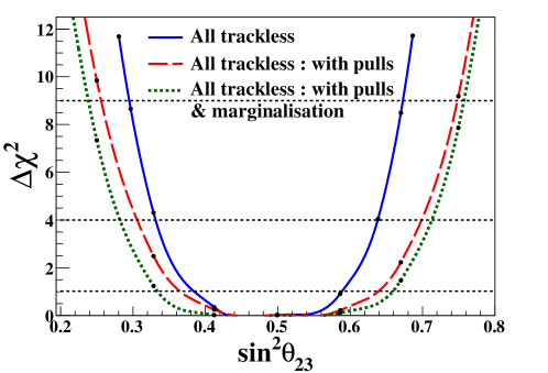
Figure 15: $\Delta\chi^{2}$ as a function of $\sin^{2}\theta_{23}$ for all trackless events without pulls (blue solid lines), with pulls (red dashed lines) and with pulls after marginalisation (green dotted lines).

VI Discussions and Conclusions

Simulation studies of charged-current atmospheric muon neutrino events, CC$\mu$, in the ICAL detector have established its capability to precisely determine the so-called atmospheric parameters $\theta_{23}$ and $\Delta m_{32}^{2}$, including its sign (the neutrino mass ordering issue) through the observation of earth matter effects in neutrino (and anti-neutrino) oscillations. In this paper, for the first time, we consider the contribution to the sensitivity to atmospheric neutrino oscillation parameters from trackless events in the ICAL detector where no track (typically assumed to be a muon) could be reconstructed. Such events arise from charged current electron and muon events as well as from neutral current interactions in the detector.

We used a simulated sample generated by the NUANCE neutrino generator, which corresponds to 100 years (or equivalently to 5000 kton-years) of data, in which the response of ICAL is modelled by GEANT4. Using pure CC$e$ events, we first studied the simulation response of an ICAL-like detector with electron separation capability to CC$e$ events and showed that the detector is capable of reconstructing the energy and direction of the final state shower (of the combined electron and hadrons in the final state) with reasonable accuracy and efficiency. These reconstructed observables are then used in a $\chi^{2}$ analysis. It is shown that there was sufficient sensitivity to $\theta_{23}$.

However, it turns out that the ICAL will not be able to cleanly separate CC$e$ events (containing both electron and hadrons in the final state) from NC events (with only hadrons in the final state) or CC$\mu$ events (where the muon track failed to be reconstructed). While various selection criteria are applied, in particular, the number of hits per layer, to try and improve the discrimination to electron events, these requirements led to worse sensitivities to the oscillation parameters, since the analysis is statistics dominated. We therefore analyze the total collection of so-called “trackless events” arising from CC$e$, CC$\mu$ and NC events. The increased statistics as well as the known sensitivity of CC$\mu$ events to oscillation parameters changed the sensitivity to $\sin^{2}\theta_{23}$ significantly. We summarize our results in Table 2 where we show the results when the events are binned in the polar angle $\cos\theta$ alone; we also show that there is hardly any change in sensitivity when we include energy binning as well.

In summary, neutrino experiments are low counting experiments and hence it is important to reconstruct and analyse all possible events in neutrino detectors. A first study of the sub-dominant trackless events at the proposed ICAL detector at INO indicates that these will be sensitive to $\theta_{23}$ and hence need to be considered as well.

Binning in $\cos\theta_{\rm reco}$	Relative $1\sigma$ precision
	on $\sin^{2}\theta_{23}$
CC$e$	20%
All trackless	15%
All trackless, including systematics and marginalization	21%

Table 2: Sensitivity to $\sin^{2}\theta_{23}$ for pure CC$e$ events, all trackless events and all trackless events with systematic uncertainties.

Acknowledgements

: We thank Gobinda Majumder and Asmita Redij for developing the ICAL detector simulation packages.

References

- (1) B. Pontecorvo, J. Exp. Theor. Phys. 34, 247 (1958); Z. Maki, M. Nakagawa, and S. Sakata, Prog. Theor. Phys. 28, 870 (1962).
- (2) A. Gando et al. (KamLAND Collaboration), Phys. Rev. D 88, 033001 (2013).
- (3) K. Abe et al. (Super-Kamiokande Collaboration), Phys. Rev. D94, 052001 (2016).
- (4) F. An et al. (Daya Bay Collaboration),Phys. Rev. D 95, 072006 (2017).
- (5) Y. Abe et al. (Double Chooz Collaboration), JHEP 1601 (2016) 163.
- (6) J. H. Choi et al., (RENO Collaboration) , Phys. Rev. Lett. 116, 211801 (2016).
- (7) M. Tanabashi et al. (Particle Data Group), Phys. Rev. D 98, 030001 (2018) and 2019 update.
- (8) S. Adrián-Martínez, et al. (KM3NeT collaboration), JHEP 1705 (2017) 008.
- (9) M. G. Aartsen et al., (IceCube Collaboration) Phys. Rev. Lett. 120, 071801 (2018).
- (10) B. Abi et al. (DUNE Collaboration), arXiv:1807.10334.
- (11) I. Esteban et al., JHEP 1808 (2019) 180.
- (12) S. Ahmed et al. (ICAL Collaboration), Pramana 88, 79 (2017).
- (13) T. Thakore, A. Ghosh, S. Choubey and A. Dighe, JHEP 1305 (2013) 058.
- (14) A. Ghosh, T. Thakore and S. Choubey, JHEP 1304 (2013) 009.
- (15) M.-M. Devi, T. Thakore, S. K. Agarwalla and A. Dighe, JHEP 1410 (2014) 189.
- (16) L. S. Mohan and D. Indumathi, Eur. Phys. J. C 77, 54 (2017).
- (17) L. S. Mohan et al., JINST 9 (2014) T09003.
- (18) M.-M. Devi et al., JINST 8 (2013) P11003.
- (19) M.-M. Devi et al., JINST 13 (2018) C03006.
- (20) S. Agostinelli et al. (GEANT4 collaboration), Nucl. Instrum. Meth. A 506, 250 (2003).
- (21) J. Allison et al., IEEE Trans. Nucl. Sci. 53, 270 (2006).
- (22) D. Casper, Nucl. Phys. Proc. Suppl. 112, 161 (2002).
- (23) D. Indumathi, M.V.N. Murthy, G.Rajasekaran and N. Sinha, Phys. Rev. D 74, 053004 (2006).
- (24) C. Patrignani et al., Chin. Phys. C, 40, 100001 (2016) and 2017 update.
- (25) M. Honda, T. Kajita, K. Kasahara and S. Midorikawa, Phys. Rev. D 83, 123001 (2011).
- (26) G. Rajasekaran, AIP Conference proceedings (Ed. Adam Para) Volume 721, 243 (2004).
- (27) S. R. Dugad, Proc. Indian Natn. Sci. Acad. 70,A, 39 (2004).
- (28) R. E. Kalman, Trans. ASME J. Basic Eng. 82, 35 (1960).
- (29) L. S. Mohan, Precision measurement of neutrino oscillation parameters at INO ICAL, PhD thesis, 2014.
- (30) M.C. Gonzalez-Garcia and M. Maltoni, Phys. Rev. D 70, 033010 (2004).
- (31) G. L. Fogli et al., Phys. Rev. D 66, 053010 (2002).
- (32) K. R. Rebin, J. Libby, D. Indumathi, L. S. Mohan, Eur. Phys. J. C79, 295 (2019).