Reduced order methods for parametrized non-linear and time dependent optimal flow control problems, towards applications in biomedical and environmental sciences

Abstract

We introduce reduced order methods as an efficient strategy to solve parametrized non-linear and time dependent optimal flow control problems governed by partial differential equations. Indeed, the optimal control problems require a huge computational effort in order to be solved, most of all in physical and/or geometrical parametrized settings. Reduced order methods are a reliable and suitable approach, increasingly gaining popularity, to achieve rapid and accurate optimal solutions in several fields, such as in biomedical and environmental sciences. In this work, we employ a POD-Galerkin reduction approach over a parametrized optimality system, derived from the Karush-Kuhn-Tucker conditions. The methodology presented is tested on two boundary control problems, governed respectively by (i) time dependent Stokes equations and (ii) steady non-linear Navier-Stokes equations.

1 Introduction

Parametrized optimal flow control problems (OFCP($\bm{\mu}$)s) constrained to parametrized partial differential equations (PDE($\bm{\mu}$)s) are a very versatile mathematical model which arises in several applications, see e.g. [7, 9, 4]. These problems are computationally expensive and challenging even in a simpler non-parametrized context. The computational cost becomes unfeasible when these problems involve time dependency [1, 14] or non-linearity [5, 6, 4], in addition to physical and/or geometrical parametrized settings that describe several configurations and phenomena. A suitable strategy to lower this expensive computational effort is to employ reduced order methods (ROMs) in the context of OCP($\bm{\mu}$)s, which recast them in a cheap, yet reliable, low dimensional framework [8, 12]. We exploit these techniques in order to solve boundary OCP($\bm{\mu}$)s on a bifurcation geometry [13] which can be considered as (i) a riverbed in environmental sciences and as (ii) a bypass graft for cardiovascular applications. In the first research field, reduced parametrized optimal control framework (see e.g. [10, 11]) can be of utmost importance. It perfectly fits in forecasting and data assimilated models and it could be exploited in order to prevent possibly dangerous natural situations [15]. The presented test case is governed by time dependent Stokes equations, which are an essential tool in marine sciences in order to reliably simulate evolving natural phenomena.
Furthermore, discrepancies between computational modelling in cardiovascular mechanics and reality usually ought to high computational cost and lack of optimal quantification of boundary conditions, especially the outflow boundary conditions. In this work, we present application of the aforementioned numerical framework combining OFCP($\mu$) and reduced order methods in the bifurcation geometry. The aim is to quantify the outflow conditions automatically while matching known physiological data for different parameter-dependent scenarios [2, 17]. In this test case, Navier-Stokes equations will model the fluid flow.

The work is outlined as follows: in section 2, the problem formulation and the methodology are summarized. Section 3 shows the numerical results for the two boundary OCP($\bm{\mu}$)s, based on [9, 13]. Conclusions follow in section 4.

2 Proper Orthogonal Decomposition for OCP($\bm{\mu}$)s

In this section, we briefly describe the problem and the adopted solution strategy for time dependent non-linear boundary OCP($\bm{\mu}$)s: in the cases mentioned in section 1, the reader shall take the non-linear term and time-dependent terms to be zero accordingly [16, 17]. The goal of OCP($\bm{\mu}$)s is to find a minimizing solution for a quadratic cost functional $\mathcal{J}$ under a PDE($\bm{\mu}$) constraint thanks to an external variable denoted as control. In the next section, we will show numerical results over a bifurcation geometry $\Omega$ with physical and/or geometrical parametrization represented by $\boldsymbol{\mu}\in\mathcal{D}\subset\mathbb{R}^{d},d\in\mathbb{N}$. Thus, considering the space-time domain $Q=\Omega\times[0,T]$ with a sufficiently regular spatial boundary $\partial\Omega$ , let us define the Hilbert spaces $S=V\times P$, $Z=Z_{V}\times Z_{P}$ and $U$ for state and adjoint velocity and pressure, and control variables denoted by $\boldsymbol{s}=\left(\boldsymbol{v},p\right)\in S$, $\boldsymbol{u}\in U$ and $\boldsymbol{z}=\left(\boldsymbol{w},q\right)\in Z$, respectively. The stability and uniqueness of the optimal solution will be guaranteed if $S\equiv Z$, which will be our assumption in this work. We introduce $X=S\times U$ such that $\mathbf{x}=\left(\boldsymbol{s},\boldsymbol{u}\right)\in X$. Then, the problem reads: given $\boldsymbol{\mu}\in\mathcal{D}$ , find $\left(\mathbf{x},\boldsymbol{z};\boldsymbol{\mu}\right)\in X\times S$ s.t.:

$$\begin{cases}\begin{matrix}\mathcal{A}\left(\mathbf{x},\mathbf{y};\boldsymbol{\mu}\right)+\mathcal{B}\left(\boldsymbol{z},\mathbf{y};\boldsymbol{\mu}\right)\ +\\ \mathcal{E}\left(\boldsymbol{v},\boldsymbol{w},\mathbf{y}_{\boldsymbol{v}};\boldsymbol{\mu}\right)+\mathcal{E}\left(\boldsymbol{w},\boldsymbol{v},\mathbf{y}_{\boldsymbol{v}};\boldsymbol{\mu}\right)\end{matrix}=\int_{0}^{T}\left\langle\mathcal{H}\left(\boldsymbol{\mu}\right),\mathbf{y}\right\rangle dt,&\ \forall\ \mathbf{y}\in X,\\ \mathcal{B}\left(\mathbf{x},\boldsymbol{\kappa};\boldsymbol{\mu}\right)+\mathcal{E}\left(\boldsymbol{v},\boldsymbol{v},\boldsymbol{\kappa}_{\boldsymbol{w}};\boldsymbol{\mu}\right)=\int_{0}^{T}\left\langle\mathcal{G}\left(\boldsymbol{\mu}\right),\boldsymbol{\kappa}\right\rangle dt,&\ \forall\ \boldsymbol{\kappa}\in S,\end{cases}$$ (1)

where $\mathbf{y}=\left(\mathbf{y}_{\boldsymbol{v}},\mathbf{y}_{p},\mathbf{y}_{\boldsymbol{u}}\right)$ and $\boldsymbol{\kappa}=(\boldsymbol{\kappa}_{\boldsymbol{w}},\boldsymbol{\kappa}_{q})$. The bilinear forms $\mathcal{A}:X\times X\rightarrow\mathbb{R}$ and $\mathcal{H}\left(\boldsymbol{\mu}\right)$ are related to the minimization cost functional $\mathcal{J}$, while the bilinear form $\mathcal{B}:X\times Z\rightarrow\mathbb{R}$ represents the linear part of state-constraints and $\mathcal{E}$ is the non-linear convection term, which will be zero for the time dependent linear case.
In order to solve the optimality system (1) we exploit Galerkin Finite Elements (FE) snapshots-based Proper orthogonal decomposition (POD)–Galerkin (see [8]), summarized in table 1, where the number of time steps are denoted by $\mathcal{N}_{t}$.

Offline phase:                                                        Input: $\mu_{1}$ for lifting, $N$, $n$.
Output: Reduced order solution spaces.
$1.$ Compute snapshots $\bm{\delta}_{\mathcal{N}_{\bm{\delta}}\times\mathcal{N}_{t}}\left(\bm{\mu}^{n}\right)$ for $1\leq n\leq|\Lambda|,\ \bm{\delta}=\bm{v},p,\bm{u},\bm{w},q$ and state and adjoint
supremizers. The global dimension of FE space discretization is $\mathcal{N}=2\mathcal{N}_{\bm{v}}+2\mathcal{N}_{p}+\mathcal{N}_{\bm{u}}$.
$2.$ Solve eigenvalue problems $\mathbb{A}^{\bm{\delta}}\bm{\rho}^{\bm{\delta}}_{n}=\lambda_{n}^{\bm{\delta}}\bm{\rho}^{\bm{\delta}}_{n},\ n=1,\cdots,|\bm{\Lambda}|$, where $\mathbb{A}^{\bm{\delta}}$ is correlation
matrix of snapshots.
$3.$ If relative energy of eigenvalues is greater than $1-\epsilon_{tol},\ 0<\epsilon_{tol}\ll 1$, keep corresponding
eigenvalue-eigenvector pairs $\left(\lambda^{n},{\bm{\rho}}^{n}\right)$.
$4.$ Construct orthonormal POD basis from the retained $N$ eigenvectors and add the POD modes
of the supremizers to state and adjoint velocities.
Online phase:                                                        Input: Online parameter $\bm{\mu}\in\mathcal{D}$.
Output: Reduced order solution.
$1.$ Perform Galerkin projection to calculate reduced order coefficients such that $\boldsymbol{\delta}\approx{\mathfrak{X}}_{\boldsymbol{\delta}}\boldsymbol{\delta}_{\mathrm{N}}$
where, $\mathfrak{X}_{\boldsymbol{\delta}}$ denotes reduced bases matrices containing all the time instances.
$2.$ Solve the reduced order version of the optimality system (1).

Table 1: Algorithm: POD–Galerkin for OCP($\bm{\mu}$)

In order to guarantee the efficiency of the POD–Galerkin approach, we rely on the affine assumption over the forms, i.e. every form can be written as a linear combination of $\small\bm{\mu}-$dependent functions and $\small\bm{\mu}-$independent quantities. In this way, the system resolution is divided into parameter independent (offline) and dependent (online) phases (see table 1 for details) such that the expensive calculations are absorbed in the former stage and only online stage is repeated every time the parameter $\boldsymbol{\mu}$ changes. From the perspective of the problem stability, to ensure uniqueness of pressure at the reduced order level, we enrich the state and adjoint velocity space with supremizers and, to guarantee the fulfillment of Brezzi’s inf-sup condition [3] at the reduced level, we use aggregated equivalent state and adjoint spaces. Thus, dimension of the reduced problem reduces from $\mathcal{N}\times\mathcal{N}_{t}$ to $13N$.

3 Results

3.1 Linear Time Dependent OCP($\bm{\mu}$)  governed by Stokes Equations

In this section, inspired by [9, 13], we propose an OFCP($\boldsymbol{\mu}$) governed by a time dependent Stokes equation. First of all, let us introduce the smooth domain $\Omega(\mu_{2})$. The parameter stretches the length of the reference domain shown in figure 2, which will be indicated with $\Omega$ from now on. We want to recover a measurement $\boldsymbol{v}_{d}(\mu_{3})\in L^{2}(0,T;[L^{2}(\Omega)]^{2})$ over the one dimensional observation domain $\Gamma_{OBS}$ controlling the Neumann flux over $\Gamma_{C}$, with the inflow $\bm{v}_{{in}}\left(\bm{\mu}\right)=(10\left(x_{2}-1)\left(1-x_{2}\right),0\right)$. The setting is suited for environmental applications: we control the flow in order to avoid potentially dangerous situations in an hypothetical real time monitoring plan on the domain, which can represent a riverbed. The space-time domain is $Q=\Omega\times[0,1]$. Let us consider the following function spaces: $V=L^{2}(0,T;[H^{1}_{\Gamma D}(\Omega)]^{2})\cap H^{1}(0,T;[H^{1}_{\Gamma D}(\Omega)^{\ast}]^{2})$, $P=L^{2}(0,T;L^{2}(\Omega))$ and $U=L^{2}(0,T;[L^{2}(\Omega)]^{2})$ for state and adjoint velocity, state and adjoint pressure and for control, respectively. Then, we define $X=(V\times P)\times U$. For a given $\bm{\mu}\in\mathcal{D}=[0.01,1]\times[1,2]\times[0.01,1]$, we want to find the solution of time dependent Stokes equations which minimizes:

$$\small\mathcal{J}:=\frac{1}{2}\int_{0}^{T}\int_{\Gamma_{OBS}}(\boldsymbol{v}(\bm{\mu})-\boldsymbol{v}_{d}(\mu_{3}))^{2}dsdt+\frac{\alpha_{1}}{2}\int_{0}^{T}\int_{\Gamma_{C}}\boldsymbol{u}(\bm{\mu})^{2}dsdt+\frac{\alpha_{2}}{2}\int_{0}^{T}\int_{\Gamma_{C}}|\nabla\boldsymbol{u}(\bm{\mu})\boldsymbol{t}|^{2}dsdt,$$ (2)

where $\alpha_{1}=10^{-3},\alpha_{2}=10^{-4}$ and $\boldsymbol{t}$ is the unit tangent vector to $\Gamma_{C}$ and $\boldsymbol{v}_{d}(\mu_{3})=[\mu_{3}(8(x_{2}^{3}-x_{2}^{2}-x_{2}+1)+2(-x_{2}^{3}-x_{2}^{2}+x_{2}+1)),0]$. The cost functional penalizes not only the magnitude of the control, but also its rapid variations over the boundary. The constrained minimization problem (2) is equivalent to the resolution of problem (1) where the considered forms are defined by:

$$\small\mathcal{A}(\mathbf{x},\mathbf{y}) =\int_{0}^{T}\int_{\Gamma_{OBS}}\boldsymbol{v}\cdot\mathbf{y}_{\boldsymbol{v}}\;dsdt+\alpha_{1}\int_{0}^{T}\int_{\Gamma_{C}}\boldsymbol{u}\cdot\mathbf{y}_{\boldsymbol{u}}\;dsdt+\alpha_{2}\int_{0}^{T}\int_{\Gamma_{C}}\nabla\boldsymbol{u}\boldsymbol{t}\cdot\nabla\mathbf{y}_{\boldsymbol{u}}\boldsymbol{t}\;dsdt,$$

$$\mathcal{B}(\mathbf{x},\bm{z};\bm{\mu}) =\int_{Q}{\frac{\partial\boldsymbol{v}}{\partial t}\cdot\bm{w}\;dxdt}+\mu_{1}\int_{Q}{\nabla{\boldsymbol{v}}\cdot\nabla{\bm{w}}\;dxdt}-\int_{Q}{p(\nabla\cdot\bm{w}(\bm{\mu}))}\;dxdt$$

$$\qquad\qquad\qquad-\int_{Q}{q(\nabla\cdot{(\bm{v}(\bm{\mu}))}\;dxdt}-\int_{0}^{T}\int_{\Gamma_{C}}{\boldsymbol{u}\cdot\bm{w}\;dsdt},$$

$$\langle\mathcal{H}(\bm{\mu}),\mathbf{y}\rangle =\int_{\Gamma_{OBS}}\boldsymbol{v}_{d}(\mu_{3})\cdot\mathbf{y}_{\boldsymbol{v}}\;ds,\qquad\langle\mathcal{G}(\bm{\mu}),{q}\rangle=0,\;\;\;\forall\mathbf{y}\in X,\vspace{-1.7cm}$$

for every $\mathbf{x},\mathbf{y}\in X$ and $\bm{\kappa}\in S$. We built the reduced space with $N=35$ over a training set of $70$ snapshots of global dimension $131400$, for $\mathcal{N}_{t}=20$. In time dependent applications, ROMs are of great advantage: in table 2 the speedup index is shown with respect to $N$. The speedup represents how many ROM systems one can solve in the time of a FE simulation. Nevertheless, we do not pay in accuracy as figure 1 and figure 3 show: it represents the relative error between FE and ROM variables. The relative error between FE and ROM $\mathcal{J}$ is presented in table 2

Table 2: Speedup analysis and relative error $\mathcal{J}$.

$N$	Speedup	Relative error $\mathcal{J}$
$15$	$\;66338$	$\qquad 10^{-7}$
$20$	$\;47579$	$\qquad 10^{-8}$
$25$	$\;34335$	$\qquad 10^{-8}$
$30$	$\;22477$	$\qquad 10^{-9}$
$35$	$\;17420$	$\qquad 10^{-10}$

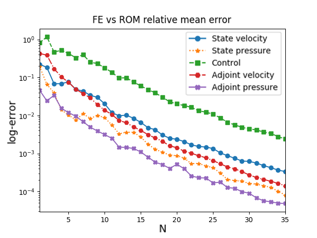
Figure 1: FE vs ROM mean relative error over 50 parameters.

Figure 2: Physical domain.

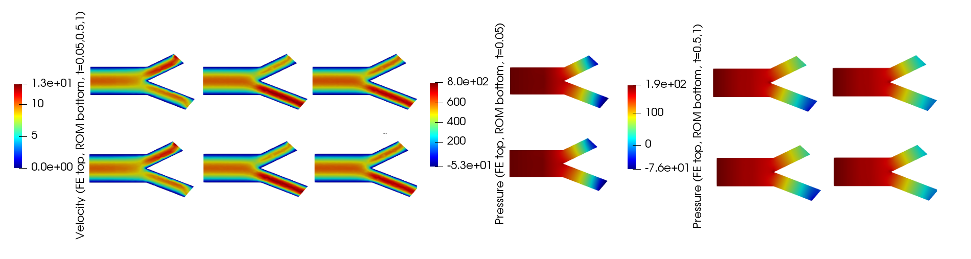
Figure 3: FE (top) vs ROM (bottom) comparison of state velocity and state pressure, for t=0.05,0.5,1 and $\bm{\mu}=(0.5,1.5,1)$.

3.2 Non-linear steady OCP($\bm{\mu}$)  governed by Navier-Stokes equations

In this section, we will demonstrate the numerical results for second test case with optimal boundary control problem governed by non-linear incompressible steady Navier-Stokes equations. We consider a bifurcation domain $\Omega$ as employed in the previous example (see figure 5), which can be considered as an idealized model of arterial bifurcation in cardiovascular problems [9, 13, 17]. Fluid shall enter the domain from $\Gamma_{in}$ and shall leave through the outlets $\Gamma_{c}$. In this example, physical parameterization is considered for the inflow velocity given by $\bm{v}_{{in}}\left(\bm{\mu}\right)=10{\mu}_{1}\left(x_{2}\left(2-x_{2}\right),0\right)$ and the desired velocity, denoted by $\bm{v}_{d}\in L^{2}\left(\Omega\right)$ and prescribed at the 1-D observation boundary $\Gamma_{obs}$ through the following expression:

$$\small\bm{v}_{d}\left(\bm{\mu}\right)=\begin{pmatrix}10\mu_{1}\left(0.8\left(\left(x_{2}-1\right)^{3}-\left(x_{2}-1\right)^{2}-\left(x_{2}-1\right)+1\right)+0.2\left(-\left(x_{2}-1\right)^{3}-\left(x_{2}-1\right)^{2}+x_{2}\right)\right)\\ 0\end{pmatrix}.$$

The cost-functional $\mathcal{J}$ is defined as:

$$\small\mathcal{J}\left(\bm{v},\bm{u};\bm{\mu}\right)=\frac{1}{2}\|\bm{v}\left(\bm{\mu}\right)-\bm{v}_{d}\left(\bm{\mu}\right)\|^{2}_{L^{2}\left(\Gamma_{obs}\right)}+\frac{\alpha}{2}\|\bm{u}\left(\bm{\mu}\right)\|^{2}_{L^{2}\left(\Gamma_{c}\right)}\\ +\frac{0.1\alpha}{2}\|\nabla\bm{u}\left(\bm{\mu}\right)\bm{t}\|^{2}_{L^{2}\left(\Gamma_{c}\right)},$$ (3)

where $\bm{t}$ is the tangential vector to $\Gamma_{c}$. The mathematical problem reads: Given $\bm{\mu}\in\mathcal{D}=\left[0.5,1.5\right]$, find $\left(\bm{v}\left(\bm{\mu}\right),p\left(\bm{\mu}\right),\bm{u}\left(\bm{\mu}\right)\right)$ that minimize $\mathcal{J}$ and satisfy the Navier-Stokes equations with $\bm{v}_{{in}}\left(\bm{\mu}\right)$ prescribed at the inlet $\Gamma_{{in}}$, no-slip conditions at the walls $\Gamma_{w}$ and $\bm{u}\left(\bm{\mu}\right)$ implemented at $\Gamma_{c}$ through Neumann conditions.

At the continuous level, we consider $X\left(\Omega\right)=H^{1}_{\Gamma_{in}\cup\Gamma_{w}}\left(\Omega\right)\times L^{2}\left(\Omega\right)\times L^{2}\left(\Gamma_{c}\right)$, where

$$\small H^{1}_{\Gamma_{in}\cup\Gamma_{w}}\left(\Omega\right)=\left[\bm{v}\in\left[H^{1}\left(\Omega\right)\right]^{2}:\bm{v}|_{\Gamma_{{in}}}=\bm{v}_{{in}}\ \text{and}\ \bm{v}|_{\Gamma_{w}}=0\right].$$

Thus,

$$\mathcal{A}\left(\mathbf{x},\bm{y}\right) =\int_{\Omega}\bm{v}\left(\bm{\mu}\right)\cdot\bm{y}_{\bm{v}}d\Omega+\alpha\int_{\Gamma_{c}}\bm{u}\left(\bm{\mu}\right)\cdot\bm{y}_{\bm{u}}d\Gamma_{c}+\frac{\alpha}{10}\int_{\Gamma_{c}}\left(\nabla\bm{u}\left(\bm{\mu}\right)\right)\bm{t}\cdot\nabla\left(\bm{y}_{\bm{u}}\right)\bm{t}d\Gamma_{c},$$

$$\mathcal{B}\left(\mathbf{x},\bm{z}\right) =\eta\int_{\Omega}\nabla\bm{v}\left(\bm{\mu}\right)\cdot\nabla\bm{w}d\Omega-\int_{\Omega}p\left(\bm{\mu}\right)\left(\nabla\cdot\bm{w}\right)d\Omega-\int_{\Omega}q\left(\nabla\cdot\bm{v}\left(\bm{\mu}\right)\right)d\Omega$$

$$-\int_{\Gamma_{c}}\bm{u}\left(\bm{\mu}\right)\cdot\bm{w}d\Gamma_{c},$$

$$\mathcal{E}\left(\bm{v},\bm{v},\bm{w}\right) =\int_{\Omega}\left(\bm{v}\left(\bm{\mu}\right)\cdot\nabla\right)\bm{v}\left(\bm{\mu}\right)\cdot\bm{w}d\Omega\quad\text{and}\quad\left\langle\mathcal{H}\left(\bm{\mu}\right),\mathbf{y}\right\rangle=\int_{\Omega}\bm{v}_{d}\left(\bm{\mu}\right)\cdot\bm{y}_{\bm{v}}d\Omega.$$

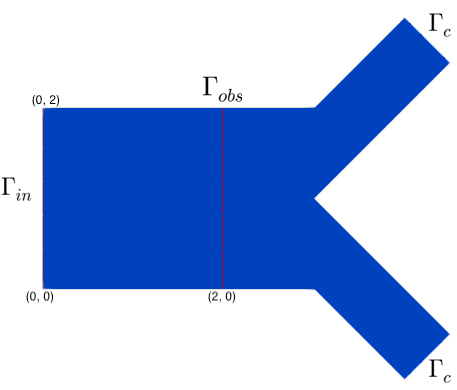
Figure 4: Domain $\left(\Omega\right)$.

Mesh size	$5977$
No. of reduced order bases $N$	$131$
$\mathcal{D}$	$\left[0.7,1.5\right]$
$|\Lambda|$	$100$
offline phase	$4.9\times 10^{3}$ seconds
online phase	$9\times 10^{1}$ seconds

Figure 5: Computational details of POD–Galerkin for Navier-Stokes constrained OCP($\bm{\mu}$).

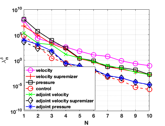
Figure 6: Eigenvalues of $\mathrm{N}=10$ POD modes.

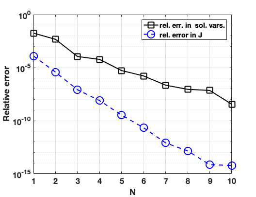
Figure 7: Relative error for solution variables and $\mathcal{J}$.

$|\bm{v}|$
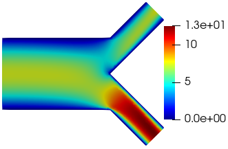
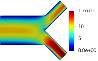
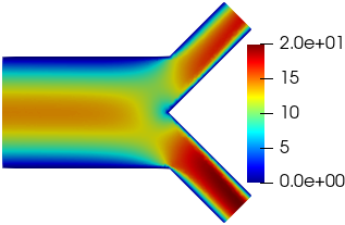
$|\bm{u}|$

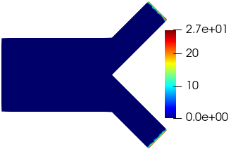
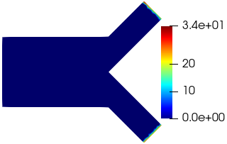
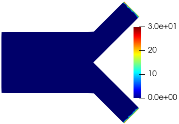
Figure 8: State velocity and control for $\mu_{1}=0.7,1.1,1.4$.

To construct the reduced order solution spaces, we consider a sample $\left(\Lambda\right)$ of $100$ parameter values and solving the problem (1) through Galerkin Finite Element method, we construct the snapshot matrices for the solution variables $\bm{v},p,\bm{u},\bm{w},q$. For $N=10$, eigenvalues energy of the state, control and adjoint variables is demonstrated in figure 7. Evidently, $N$ eigenvalues capture $99.9\%$ of the Galerkin FE discretized solution spaces and the reduced order spaces are thus built with dimensions $13\mathrm{N}+1=131$. The state velocity and control for $\mu=0.7,1.1,1.4$ are shown in figure 8. Furthermore, we report the accumulative relative error for the solution variables and the relative error for $\mathcal{J}$ in figure 7. The former decreases upto $10^{-8}$ along with the latter decreasing upto $10^{-14}$.

4 Concluding Remarks

In this work, we propose ROMs as a suitable tool to solve a parametrized boundary OCP($\bm{\mu}$)s for time dependent Stokes equations and steady Navier-Stokes equations. The framework proposed is suited for several many query and real time applications both in environmental marine sciences and bio-engineering. The reduction of the KKT system is performed through a POD-Galerkin approach, which leads to accurate surrogate solutions in a low dimensional space. This work aims at showing how ROMs can have an effective impact in the management of parametrized simulations for social life and activities, such as coastal engineering and cardiovascular problems. Indeed, the proposed framework deals with faster solving of parametrized optimal solutions which can find several applications in monitoring planning both in marine ecosystems and patient specific geometries.

References

- [1] V. Agoshkov, A. Quarteroni, and G. Rozza. A mathematical approach in the de-sign of arterial bypass using unsteady stokes equations. Journal of Scientific Computing, 2006.
- [2] F. Ballarin, E. Faggiano, S. Ippolito, A. Manzoni, A. Quarteroni, G. Rozza, and R. Scrofani. Fast simulations of patient-specific haemodynamics of coronary artery bypass grafts based on a pod–galerkin method and a vascular shape parametrization. Journal of Computational Physics, 315:609–628, 2016.
- [3] F. Brezzi. On the existence, uniqueness and approximation of saddle-point problems arising from Lagrangian multipliers. Revue française d’automatique, informatique, recherche opérationnelle. Analyse numérique, 8(2):129–151, 1974.
- [4] J. C. De los Reyes and F. Tröltzsch. Optimal control of the stationary Navier-Stokes equations with mixed control-state constraints. SIAM Journal on Control and Optimization, 46(2):604–629, 2007.
- [5] A. V. Fursikov, M. D. Gunzburger, and L. Hou. Boundary value problems and optimal boundary control for the Navier–Stokes system: the two-dimensional case. SIAM Journal on Control and Optimization, 36(3):852–894, 1998.
- [6] M. D. Gunzburger, L. Hou, and Th. P. Svobodny. Analysis and finite element approximation of optimal control problems for the stationary Navier-Stokes equations with distributed and Neumann controls. Mathematics of Computation, 57(195):123–151, 1991.
- [7] J. Haslinger and R. A. E. Mäkinen. Introduction to shape optimization: theory, approximation, and computation. SIAM, Philadelphia, 2003.
- [8] J. S. Hesthaven, G. Rozza, and B. Stamm. Certified reduced basis methods for parametrized partial differential equations. SpringerBriefs in Mathematics, 2015, Springer, Milano.
- [9] F. Negri, A. Manzoni, and G. Rozza. Reduced basis approximation of parametrized optimal flow control problems for the Stokes equations. Computers & Mathematics with Applications, 69(4):319–336, 2015.
- [10] A. Quarteroni, G. Rozza, L. Dedè, and A. Quaini. Numerical approximation of a control problem for advection-diffusion processes. In IFIP Conference on System Modeling and Optimization, pages 261–273, Ceragioli F., Dontchev A., Futura H., Marti K., Pandolfi L. (eds) System Modeling and Optimization. CSMO 2005. vol 199. Springer, Boston, 2005.
- [11] A. Quarteroni, G. Rozza, and A. Quaini. Reduced basis methods for optimal control of advection-diffusion problems. In Advances in Numerical Mathematics, pages 193–216. RAS and University of Houston, 2007.
- [12] G. Rozza, D.B.P. Huynh, and A. Manzoni. Reduced basis approximation and a posteriori error estimation for Stokes flows in parametrized geometries: Roles of the inf-sup stability constants. Numerische Mathematik, 125(1):115–152, 2013.
- [13] G. Rozza, A. Manzoni, and F. Negri. Reduction strategies for PDE-constrained oprimization problems in Haemodynamics. pages 1749–1768, ECCOMAS, Congress Proceedings, Vienna, Austria, September 2012.
- [14] M. Stoll and A. Wathen. All-at-once solution of time-dependent Stokes control. J. Comput. Phys., 232(1):498–515, January 2013.
- [15] M. Strazzullo, F. Ballarin, R. Mosetti, and G. Rozza. Model reduction for parametrized optimal control problems in environmental marine sciences and engineering. SIAM Journal on Scientific Computing, 40(4):B1055–B1079, 2018.
- [16] M. Strazzullo, F. Ballarin, and G. Rozza. POD-galerkin model order reduction for parametrized time dependent linear quadratic optimal control problems in saddle point formulation. submitted. https://arxiv.org/abs/1909.09631., 2019.
- [17] Z. Zainib, F. Ballarin, G. Rozza, P. Triverio, L. Jiménez-Juan, and Fremes. S. Reduced order methods for parametric optimal flow control in coronary bypass grafts, towards patient-specific data assimilation. submitted, https://arxiv.org/abs/1911.01409., 2019.