Flash ionization signatures in the type Ibn supernova SN 2019uo

Abstract

We present photometric and spectroscopic observations of the type Ibn supernova (SN) 2019uo, the second ever SN Ibn with flash ionization (He II, C III, N III) features in its early spectra. SN 2019uo displays a rapid post-peak luminosity decline of 0.1 mag d^-1 similar to most of the SNe Ibn, but is fainter ($M^{V}_{max}=-18.30\pm 0.24$ mag) than a typical SN Ibn and shows a color evolution that places it between SNe Ib and the most extreme SNe Ibn. SN 2019uo shows P-cygni He I features in the early spectra which gradually evolves and becomes emission dominated post peak. It also shows faster evolution in line velocities as compared to most other members of the type Ibn subclass. The bolometric light curve is fairly described by a ⁵⁶Ni + circumstellar interaction model.

1 Introduction

Supernovae (SNe) undergoing interaction with a circumstellar medium (CSM) provide a unique window in the evolutionary phases of stars. Interaction, in general, produces narrow emission lines — broader than H II regions but narrower than lines arising from the outer ejecta of the supernova (Hosseinzadeh et al., 2017). However, in some cases interaction happens below the photosphere without any observable narrow emission lines (e.g. Morozova et al., 2017; Andrews & Smith, 2018). SNe IIn (Schlegel, 1990) and SNe Ia-CSM display narrow H lines indicative of interaction with a H-rich CSM. Approximately 1% of core-collapse SNe (CCSNe) show little H and narrow He features ($\sim$2000 km s^-1). With the discovery of SN 2006jc, Pastorello et al. (2007) introduced this class as SNe Ibn, whose spectral features show interaction signatures between SN ejecta and a He-rich CSM. This is defined in analogy with SNe IIn, which show narrow H features (Schlegel, 1990). SNe that are embedded in dense CSM may also show short-lived narrow high ionization emission lines ($\leq$10 days) owing to the recombination of the CSM following the shock breakout flash. These features are known as “flash features” (e.g. Gal-Yam et al., 2014). Hosseinzadeh et al. (2017) analysed a sample of SN Ibn light curves and showed that unlike SNe IIn, SNe Ibn are rather uniform in their light curve shape with rapid decay rates of 0.05–0.15 mag d^-1. SNe Ibn may have double-peaked light curves like SNe IIn, but they show a faster rise than SNe IIn (Hosseinzadeh et al., 2017). On the other hand, Pastorello et al. (2016) showed that the class is heterogeneous with many outliers: OGLE-2012-SN-006 (Pastorello et al., 2015a) has a very slow decline; LSQ13ccw (Pastorello et al., 2015b) is faint and fast-declining; SNe 2005la and 2011hw (Pastorello et al., 2015c) are transitional type IIn/Ibn events; SN 2010al (Pastorello et al., 2015c) is the earliest detected SN Ibn with a slow rise and decline. Karamehmetoglu et al. (2019) recently identified a rapid evolving SN 2018bcc. SNe Ibn have bluer continuum than other CCSNe. Some SNe Ibn show P Cygni He I emission, while others transition from narrow to intermediate-width He I emissions (Hosseinzadeh et al., 2017).

So far, only indirect progenitor constraints for SNe Ibn are available. Pastorello et al. (2007) suggest Wolf-Rayet (WR) H-free atmospheres generate the He-rich CSM. The best studied case for unstable mass loss from a WR progenitor is SN 2006jc, for which an optical transient was detected at the SN location two years prior to explosion (Foley et al., 2007; Pastorello et al., 2007; Smith et al., 2008). Alternatively, CSM can be produced by stripping material from envelopes of massive binaries (Foley et al., 2007). However, a low-mass progenitor has been suggested for PS1-12sk, which occurred in a non-star-forming host (Sanders et al., 2013; Hosseinzadeh et al., 2019) — unlikely for a CCSN ($\leq$0.2%; Hakobyan et al., 2012). A very recent study by Sun et al. (2019) for SNe 2006jc and 2015G implies an interacting binary progenitor scenario, based on late time UV/optical HST images.

In this paper we study the evolution of one such type Ibn SN 2019uo which was discovered on 2019 January 17.8 UT (JD 2458501.3) by Koichi Itagaki at $\mathrm{R.A.}=12^{\mathrm{h}}02^{\mathrm{m}}36.5^{\mathrm{s}}$, $\mathrm{Decl.}=+41\arcdeg 03^{\prime}42^{\prime\prime}$ (J2000.0). The SN location is 0$\farcs$4 east and 27$\farcs$2 north of the center of the galaxy UGC 7020 at a redshift of 0.020454 (Zhang et al., 2019). SN 2019uo was classified on 2019 January 19.9 UT as a SN II (Zhang et al., 2019) with the spectrum obtained with the Yunnan Faint Object Spectrograph and Camera (YFOSC) mounted on the 2.4 m LiJiang Telescope (LJT) at Yunnan Observatory (YNAO). Zhang et al. (2019) reported that the spectrum depicted a blue continuum and highly ionized “flash features” such as N V, He II and O V. However, this classification of type II SN was modified later by Fremling et al. (2019) and SN 2019uo was classified as a type Ibn. Prominent narrow emission lines of He I in the initial spectra of SN 2019uo indicating a P-cygni velocity of 650 km s^-1 justified the type Ibn classification. SN 2019uo is the second SN Ibn to show these features after SN 2010al. Adopting $H_{0}=73$ km s^-1 Mpc^-1, we obtain a luminosity distance of 88.8 Mpc for SN 2019uo. The Milky Way extinction along the line of sight of SN 2019uo is $A_{V}=0.035$ mag (Schlafly & Finkbeiner, 2011). For estimating the extinction along the line of sight within host galaxy, we estimate equivalent widths of the Na ID line in the first three spectra of SN 2019uo. Using the formulation by Munari & Zwitter (1997) and Poznanski et al. (2012), we estimate $A_{V}=0.2517$ mag. This estimate also brings the $B-V$ colors of SN 2019uo into close agreement with SNe 2006jc and 2010al. Thus, we adopt a total $A_{V}=0.287$ mag. The temporal and spectral evolution of SN 2019uo and the detailed modeling of the bolometric light curve is discussed in the sections to follow.

Table 1: Photometry of SN 2019uo

Date	JD	Phase†	$U$	$B$	$g$	$V$	$r$	$i$	Telescope
(yyyy-mm-dd)	(2458000+)	(day)	(mag)	(mag)	(mag)	(mag)	(mag)	(mag)
2019-01-18	501.8	-6.8	—	17.865$\pm$0.107	17.637$\pm$0.097	17.927$\pm$0.146	17.936$\pm$0.139	—	LCO
2019-01-20	503.9	-4.7	16.452$\pm$0.033	16.937$\pm$0.027	16.785$\pm$0.013	17.052$\pm$0.026	17.039$\pm$0.019	17.353$\pm$0.033	LCO
2019-01-20	504.3	-4.3	—	16.817$\pm$0.052	16.908$\pm$0.162	17.262$\pm$0.050	—	17.423$\pm$0.052	TNT
2019-01-21	505.3	-3.3	—	16.623$\pm$0.013	16.768$\pm$0.018	17.014$\pm$0.030	16.901$\pm$0.029	17.328$\pm$0.038	TNT
2019-01-21	505.2	-3.4	—	—	—	16.882$\pm$0.08	—	—	0.7m
2019-01-22	506.2	-2.4	—	—	—	16.777$\pm$0.063	—	—	0.7m
2019-01-23	506.8	-1.8	16.122$\pm$0.074	—	16.613$\pm$0.039	16.883$\pm$0.051	—	—	LCO
2019-01-23	507.3	-1.3	—	16.654$\pm$0.036	16.699$\pm$0.022	16.991$\pm$0.034	16.821$\pm$0.034	17.187$\pm$0.042	LCO
2019-01-24	507.8	-0.8	16.252$\pm$0.075	16.731$\pm$0.031	16.532$\pm$0.015	16.669$\pm$0.027	16.676$\pm$0.022	17.215$\pm$0.022	LCO
2019-01-25	508.1	-0.6	—	—	—	16.673$\pm$0.024	—	17.037$\pm$0.015	LJT
2019-01-25	508.3	-0.3	16.015$\pm$0.020	16.825$\pm$0.031	16.655$\pm$0.019	16.616$\pm$0.101	16.782$\pm$0.022	17.027$\pm$0.0272	LJT,TNT,0.7m
2019-01-25	508.8	0.1	16.199$\pm$0.051	16.740$\pm$0.026	16.565$\pm$0.017	16.685$\pm$0.028	16.654$\pm$0.023	17.003$\pm$0.055	LCO
2019-01-28	511.4	2.7	—	—	—	16.732$\pm$0.143	—	—	0.7m
2019-01-28	511.8	3.1	16.331$\pm$0.028	17.156$\pm$0.017	—	16.749$\pm$0.0153	16.646$\pm$0.010	—	DFOT
2019-01-30	513.1	4.5	—	—	—	16.786$\pm$0.085	—	—	ST
2019-02-01	515.7	7.1	17.334$\pm$0.049	17.447$\pm$0.026	17.281$\pm$0.009	17.307$\pm$0.019	17.237$\pm$0.011	17.430$\pm$0.021	LCO
2019-02-02	516.3	7.6	—	17.547$\pm$0.016	17.257$\pm$0.011	17.655$\pm$0.022	17.532$\pm$0.016	17.696$\pm$0.013	TNT
2019-02-04	518.4	9.8	—	18.275$\pm$0.016	—	—	17.847$\pm$0.017	17.948$\pm$0.014	ST
2019-02-04	518.8	10.2	18.262$\pm$0.082	18.276$\pm$0.029	17.921$\pm$0.016	17.882$\pm$0.025	17.835$\pm$0.021	17.938$\pm$0.030	LCO
2019-02-05	519.2	10.5	—	18.754$\pm$0.031	—	17.885$\pm$0.024	17.856$\pm$0.017	—	ST
2019-02-06	520.3	11.7	—	18.862$\pm$0.024	—	18.141$\pm$0.025	18.479$\pm$0.027	18.592$\pm$0.033	ST
2019-02-08	523.4	14.8	19.787$\pm$0.041	19.058$\pm$0.027	—	18.316$\pm$0.031	18.900$\pm$0.001	18.808$\pm$0.052	HCT
2019-02-09	524.4	15.7	—	19.224$\pm$0.069	—	18.598$\pm$0.029	18.911$\pm$0.037	19.091$\pm$0.033	ST
2019-02-12	527.0	18.4	—	19.487$\pm$0.053	19.169$\pm$0.037	18.946$\pm$0.043	19.012$\pm$0.048	19.136$\pm$0.075	LCO
2019-02-20	535.2	26.6	—	—	20.037$\pm$0.218	—	—	20.287$\pm$0.115	TNT
2019-02-21	536.2	27.6	—	—	20.228$\pm$0.214	—	—	—	TNT
2019-02-23	538.1	29.5	—	—	20.265$\pm$0.312	—	—	—	TNT
2019-03-02	544.3	36.2	—	21.231$\pm$0.274	20.726$\pm$0.138	20.526$\pm$0.178	21.032$\pm$0.305	21.096$\pm$0.215	LCO
† with respect to $\mathrm{JD_{max}}=2458508.65$.

2 Data Acquisition and Reduction

We observed SN 2019uo with Las Cumbres Observatory (LCO) in the UBVgri filters from $\sim$2 to 106 days after discovery. Augmenting the LCO data, photometric observations in UBVRI/ugri were also taken with 0.7m BITRAN-CCD Imaging System located in Japan; 0.8m Tsinghua-NAOC Telescope (TNT), Xinglong Observatory, China; 1.04m Sampurnanand Telescope (ST); 1.30m Devasthal Fast Optical Telescope (DFOT), ARIES, India; 2.00m Himalayan Chandra Telescope (HCT), IAO, Hanle, India and Lijiang 2.4m Telescope (LJT), Yunnan Observatories (YNAO), China. We performed image subtraction using High Order Transform of PSF ANd Template Subtraction (HOTPANTS)(Becker, 2015). The instrumental magnitudes were estimated using IRAF(Tody, 1986, 1993) and DAOPHOT(Stetson, 1987). The LCO photometry was done using lcogtsnpipe (see Valenti et al., 2011, 2016) on the difference images. The instrumental SN magnitudes were calibrated using the standard magnitudes of a number of local stars in the SN field obtained from the Sloan Digital Sky Survey (SDSS) catalog for the gri bands and the Landolt standard fields taken on the same night by the same instrument as the science images for UBV. Wherever required, the RI magnitudes were converted to ri using the equations of Jordi et al. (2006). The photometry of SN 2019uo is presented in Table 1.

Table 2: Log of spectroscopic observations of SN 2019uo.

Date	$\mathrm{JD}-2458000$	Phase†	Telescope	Instrument	Range (Å)
2019-01-19	503.4	-5.2	2.4 m LJT	YFOSC	3500-8800
2019-01-20	503.9	-4.7	2.0 m FTN	FLOYDS	3200-9000
2019-01-21	504.9	-3.7	2.0 m FTN	FLOYDS	3200-9000
2019-01-23	506.9	-1.7	2.0 m FTN	FLOYDS	3200-9000
2019-01-24	508.3	-0.3	2.4 m LJT	YFOSC	3500-8800
2019-01-28	512.4	3.8	2.0 m FTN	FLOYDS	3200-9000
2019-02-05	519.9	11.3	2.0 m FTN	FLOYDS	3200-9000
2019-02-08	523.8	15.2	2.2 m China	BFOSC	4000-10000
2019-02-14	529.2	20.6	2.4 m LJT	YFOSC	3500-8800
† with respect to $\mathrm{JD_{max}}=2458508.65$.

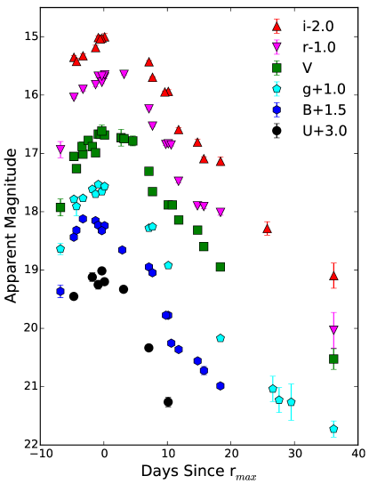
Figure 1: UBVgri light curve evolution of SN 2019uo.

The spectroscopic observations were taken at 9 epochs spanning up to $\sim$88 days after discovery. The 1D wavelength- and flux-calibrated spectra were extracted using the floydsspec pipeline (Valenti et al., 2014) for the LCO data. Spectroscopic data reduction of the 2.2 m and 2.4 m telescopes was done using the APALL task in IRAF followed by wavelength and flux calibration. The slit loss corrections were done by scaling the spectra to the photometry. Finally, the spectra were corrected for the heliocentric redshift of the host galaxy. The log of spectroscopic observations is given in Table 2.

3 Photometric Evolution of SN 2019uo

The complete multi-band light curve of SN 2019uo is shown in Figure 1. With our available observations, we were able to trace the epoch of maximum in all the bands. The date of maximum and its brightness were determined by fitting a cubic spline to the UBVgri light curves. The maximum in $r$-band occurred on JD $2458508.6\pm 0.5$ at an apparent magnitude of $16.66\pm 0.03$ mag. The errors reported are obtained from interpolated measurements around the peak. We use days since $r$-maximum ($r_{\mathrm{max}}$) as a reference epoch throughout the paper. Assuming that the discovery date is close to explosion, we estimated a rise time of $8.7\pm 1.3$ days. This is similar to iPTF14aki and iPTF15akq (c.f. Table 4; Hosseinzadeh et al., 2017).

The $r$-band light curve, between 0–36 days, decays with a rate of $0.126\pm 0.005$ mag d^-1. The $g$, $B$, $V$ and $i$ bands follow approximately the same decline rate. The sample of SNe Ibn in Hosseinzadeh et al. (2017) are fast-evolving with a typical decline rate of 0.1 mag d^-1 during the first month post-maximum. SN 2019uo follows the same decline rate.

Figure 2 shows the absolute magnitude light curve of SN 2019uo along with other SNe Ibn after correcting for distance and extinction. The peak $r$-band absolute magnitude of SN 2019uo is $-18.30\pm 0.24$ mag, which is at the fainter end of SN Ibn sample. The blue band in Figure 2 shows the average light curve (comprising of 95% of the SN Ibn data) of SNe Ibn taken from Hosseinzadeh et al. (2017). The average light curve was generated by using a Gaussian process to fit a smooth curve to the combined light curves on the sample of Hosseinzadeh et al. (2017). The fit was performed in log-log space to ensure consistency and smoothness between the early and late time light curves. The average light curve, thus, generated also uses the Gaussian process to fit positive and negative residuals. It is to note that SN 2019uo is $\sim$1.2 mag fainter than the normalized SNe Ibn light curve.

We compare the $B-R/r$ color evolution of SN 2019uo with a number of type Ibn SNe, which usually show heterogeneity in their color evolution. The $B-r$ color of SN 2019uo increases up to 0.64 mag $\sim$20 days post $r_{max}$, subsequently becoming blue at $\sim$36 days. Similarly, for SN 2010al and iPTF14aki the $B-r$ color increases up to $\sim$1 mag, $\sim$30 days post $R_{max}$. Thus, SN 2019uo shows a color evolution similar to SN 2010al and iPTF14aki. At similar epochs, the color evolution of SN 2006jc was extremely blue ($-0.5$ mag). SN 2006jc, then shows an overall flatter color evolution. The early blue colour are typical of type Ibn SN (Pastorello et al., 2016). The transition to redder colours for SNe 2019uo and 2010al places their behavior between SNe Ib and most extreme SNe Ibn. SN 2006jc (Pastorello et al., 2007) and OGLE-2012-SN-006 (Pastorello et al., 2015a) show redder colours post 50 days.

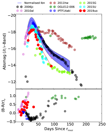
Figure 2: $R/r$-band absolute magnitude light curve and $B-R/r$ colour curve of SN 2019uo. The comparison sample includes SNe 2006jc (Pastorello et al., 2007; Foley et al., 2007), 2010al (Pastorello et al., 2015b), OGLE-SN-006 (Pastorello et al., 2015a), 2011hw (Pastorello et al., 2015b), iPTF14aki (Hosseinzadeh et al., 2017), 2015U (Shivvers et al., 2016; Hosseinzadeh et al., 2017) and 2015G (Hosseinzadeh et al., 2017).

4 Spectral evolution

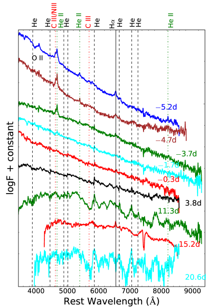
Figure 3: Spectral evolution of SN 2019uo from $-5.2$ days to 20 days post r_max. Prominent He features are seen in the early spectra. Flash ionization signatures of He II, C III and N III are also seen.

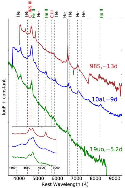
Figure 4: Spectral comparison of SN 2019uo at $-5.2$ days to SNe 1998S (Fassia et al., 2001) and 2010al (Pastorello et al., 2015b). Prominent flash ionization features are marked.

The spectral evolution of SN 2019uo from $-5.2$ days to 20.6 days post maximum is displayed in Figure 3. The early spectral sequence shows a unique blue continuum similar to SN 2010al. Blackbody fits to the first three spectra ($-5.2$, $-4.7$, and $-3.7$ days) show that the photospheric temperature varies between 13,000 K and 10,000 K. A very narrow H emission line ($\leq$137 km s^-1; unresolved) in the early spectrum of SN 2019uo is most likely due to interstellar gas in the host galaxy. Prominent emission features in the first three spectra ($-5.2$ to $-3.7$ days) of SN 2019uo are seen around $\sim$4660 Å. The emission components are double-peaked, with the blue component peaking at 4643 Å and the red component peaking at 4682 Å. The red component at 4682 Å is due to He II at 4686 Å, whereas the blue component arises from a blend of C III 4648 Å and N III 4640 Å. Another interesting feature is the possible identification of a doubly ionized C III feature at 5696 Å. Pastorello et al. (2015c) interpreted these as flash ionization signatures in a He-rich CSM (also see Gal-Yam, 2014). Although C III features were found in PTF12ldy and iPTF15ul (Hosseinzadeh et al., 2017), SN 2010al is the only previous SN Ibn where flash ionization signatures of C III and He II, typical of SNe II, are both seen. Cooke et al. (2010) and Silverman et al. (2010) identified such lines to be originating from a WR wind, previously noted in SNe IIn (e.g., SN 1998S; Fassia et al. (2001) and SN 2008fq; Taddia et al. (2013)). We also identify a He II 5411 Å feature with a velocity of 1483 km s^-1 at $-5.2$ days. In the spectrum at $-5.2$ days, we see a deep absorption feature at $\sim$4000 Å and a small dip around 8200 Å, which is likely due to the presence of O II and He II features, respectively.

Figure 4 shows the spectra of SNe 1998S (type IIn) and 2010al (type Ibn) in comparison with SN 2019uo. These two SNe have previously shown flash ionization signatures. While the spectrum of SN 2010al shows C III features around 4650 Å only, SN 2019uo shows C III features around 4650 Å and at 5696 Å. The inset in Figure 4 highlights these features.

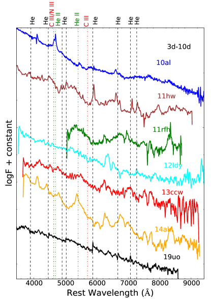
Figure 5: Comparison of the spectrum of SN 2019uo to other SNe Ibn. SN 2019uo and SN 2010al show distinct narrow P-cygni He I spectroscopic features. The data for this are taken from — SNe 2010al (Pastorello et al., 2015c), 2011hw (Pastorello et al., 2015c), PTF11rfh (Hosseinzadeh et al., 2017), PTF12ldy (Hosseinzadeh et al., 2017), LSQ13ccw (Pastorello et al., 2015b) and iPTF14aki (Hosseinzadeh et al., 2017)

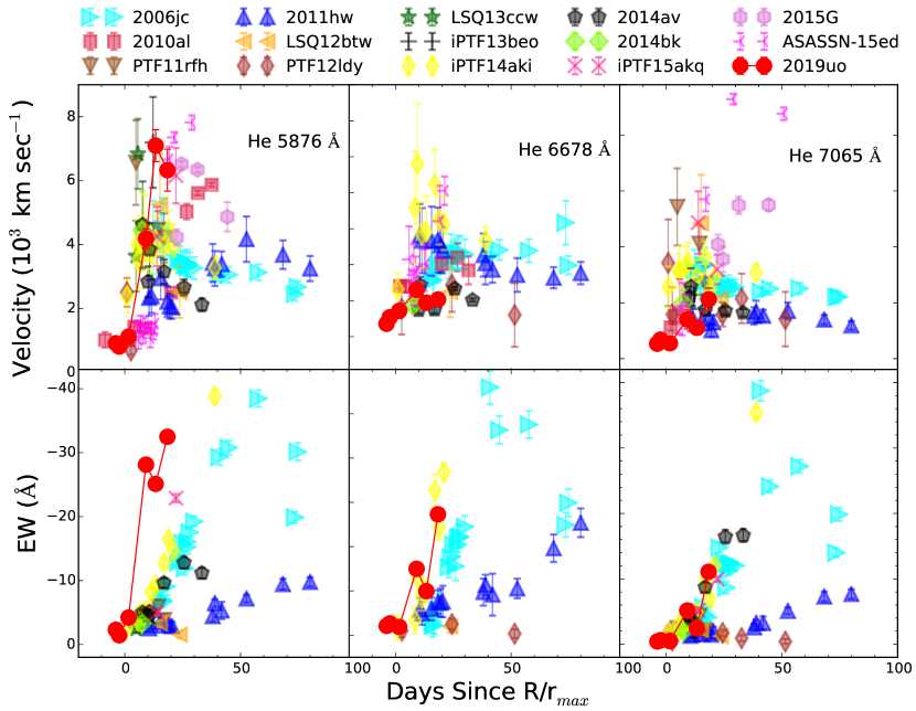
Figure 6: Evolution of line velocities and equivalent widths of He I emission lines is shown in top and bottom panels, respectively. The data for this are taken from — SNe 2006jc (Foley et al., 2007; Pastorello et al., 2008), 2010al (Pastorello et al., 2015c), 2011hw (Pastorello et al., 2015c), PTF11rfh (Hosseinzadeh et al., 2017), LSQ12btw (Pastorello et al., 2015b), OGLE12-006 (Pastorello et al., 2015a), PTF12ldy (Hosseinzadeh et al., 2017), iPTF13beo (Gorbikov et al., 2014), LSQ13ccw (Pastorello et al., 2015b), iPTF14aki (Hosseinzadeh et al., 2017), 2014av (Pastorello et al., 2016), 2014bk (Pastorello et al., 2016), iPTF15akq (Hosseinzadeh et al., 2017), ASASSN-15ed (Pastorello et al., 2015d), and 2015G (Hosseinzadeh et al., 2017).

As the SN evolves further (3.8 days), the narrow He I P Cygni feature is superimposed on a broader base (the continuum is not flat). The flash ionization spectral features vanish completely during this epoch. From 11–21 days, features of Ca II, Si II, and Na ID also start developing (see Figure 3). Figure 5 shows the comparison of SN 2019uo with a group of SNe Ibn between 3 – 10 days after peak. The He I 5876 Å feature of SN 2019uo is similar to that identified in SN 2010al. However, the He I P Cygni feature of SN 2019uo is narrower, and is superimposed over a broader emission line. On the other hand, the He I P-Cygni profile in SN 2010al is over a flat continuum. Flash ionization signatures in SN 2010al are still visible at this phase, but these features have vanished in SN 2019uo. The line evolution of SN 2019uo shows that it belongs to the “P Cygni” subclass (following the interpretation of Hosseinzadeh et al. 2017). The P Cygni He I features are narrow but gradually broaden with time. The physical explanation behind the origin of the “P Cygni” subclass could be a shell of He around the progenitor star surrounded by a dense CSM. As the optically thick shell is lit by the explosion, the narrow P Cygni features transition to broader emission as the shell is swept up by the SN ejecta. The viewing angle dependence could also affect this scenario; if the CSM is asymmetric and we have a He rich torus, then P Cygni features would only be visible if the system is viewed edge-on, while emission features can be seen only if it is viewed face-on. However, this scenario was questioned by Karamehmetoglu et al. (2019) which suggested that He I line fluxes are largely dependent on density, temperature and optical depths. Karamehmetoglu et al. (2019) suggest that dominance of emission at late phases is not because of being optically thin, but because they lack other lines to branch into it. He ionisation and recombination are mostly caused by UV and X-ray, occurring at shock boundary, deep in interacting regions. Even though most of the emission and the electron scattering are produced by the ionised region outside the shock, P-cygni features usually originate from optical depths $\leq$ 1. X-rays penetrating further into the P-cygni producing regions will fill in the absorption and lead to emission features. Thus, this provides an alternative scenario to the transitioning of P-cygni to emission features of He I lines for type Ibn SNe.

The measured the expansion velocities and equivalent widths (EWs) of three neutral He lines (5876, 6678, and 7065 Å), wherever visible. We fit the emission lines of He I using a Gaussian on a linear continuum. The EW is estimated through the integral of the flux normalized to the local continuum. We do not measure the EW of the P-cygni lines. The velocities reported are estimated from the absorption minima of P-cygni profiles. Figure 6 shows the evolution of velocity and EW for a sample of SNe Ibn taken from Hosseinzadeh et al. (2017) with time. We see that both the line velocities and EW of the He lines gradually increase with time and the velocity estimates of SN 2019uo lie in the lower range of SNe Ibn. However, SN 2019uo shows a faster evolution in line velocities, reaching broader emission profiles as seen in the P-cygni subclass (Hosseinzadeh et al., 2017) while the emission subclass shows very little velocity evolution.

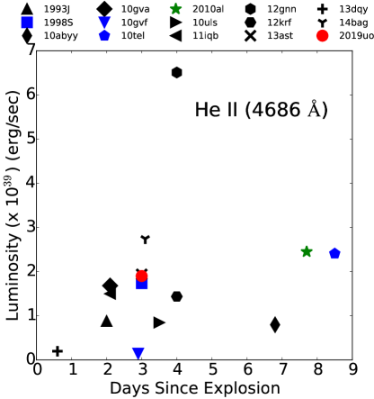
Figure 7: He II luminosity of a sample of SNe II, IIn, and Ibn (Khazov et al., 2016) with flash ionization signatures. Blue symbols: type IIn, Black symbols: type II (IIb,IIP and IIL), Red symbols: type Ibn.

To ascertain the origin of the SNe Ibn, we collected a sample of 12 SNe II (including SNe IIb and IIP, IIn) and Ibn from Khazov et al. (2016) that showed signatures of flash ionization within 10 days of explosion. Since the H lines are usually contaminated by the host galaxy, we selected the relatively unblended He II 4686 Å line. Since the He II lines are much narrower than lines from the SN ejecta, they can serve as a good tool for probing the flash-ionized CSM. When measuring the luminosities, we removed the continuum by fitting a linear function. Figure 7 shows that the typical luminosity of the He II line for SN 2019uo is similar to the type IIn SNe 1998S and PTF13ast.

5 Modeling the bolometric light curve of SN 2019uo

To construct the bolometric light curve of SN 2019uo, the measured flux values were corrected for distance and reddening as given in Section 1. Spectral energy distributions (SEDs) were constructed accounting for the flux coverage between UV to IR bands using the SuperBol (Nicholl, 2018) code. The lack of UV and NIR data was supplemented by extrapolating the SEDs using the blackbody approximation and direct integration method as described in Lusk & Baron (2017). A linear extrapolation was performed in UV regime at late times. The estimated peak bolometric luminosity of SN 2019uo is $8.9\times 10^{42}$ erg s^-1. We used different models to fit the bolometric light curve at a fixed optical opacity of 0.1 cm² g^-1. A Markov Chain Monte Carlo (MCMC) technique was used to obtain the best-fit parameters.

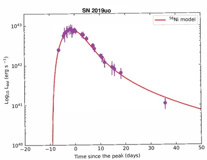
Figure 8: Best-fit light curves of SN 2019uo using a ⁵⁶Ni model.

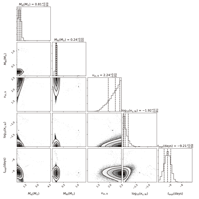
Figure 9: The corner plot of the ⁵⁶Ni model displaying covariance of estimated parameters.

⁵⁶Ni model: Assuming that the peak bolometric luminosity is powered by the decay of ⁵⁶Ni to ⁵⁶Co, we fit the bolometric light curve using ⁵⁶Ni model (Arnett, 1982, 1980). The parameters of the ⁵⁶Ni model are the ejecta mass $M_{\mathrm{ej}}$, the initial scale velocity of the ejecta $v_{\mathrm{sc}0}$, the ⁵⁶Ni mass $M_{\mathrm{Ni}}$, the gamma-ray opacity of ⁵⁶Ni decay photons $\kappa_{\gamma,\mathrm{Ni}}$ and explosion time $t_{\mathrm{expl}}$. The initial kinetic energy of the ejecta is neutrino-driven and is considered to be $E_{\mathrm{k}}=0.3M_{\mathrm{ej}}v_{\mathrm{sc}0}^{2}$. The best-fit parameters are tabulated in Table 3 and the best-fit model is displayed Fig. 8. The corner plot showing the covariance of the estimated parameters are represented in Fig. 9. We note that the ⁵⁶Ni mass obtained from the powering mechanism of Arnett (1982) are in concordance with the values quoted for several stripped envelope SNe (Lyman et al., 2016; Prentice et al., 2016, 2019). Although the ⁵⁶Ni mass inferred from the model is $\sim$ 0.24 M_⊙ which is comparable to that of normal CCSNe, the opacity for the gamma ray $\kappa_{\gamma,\mathrm{Ni}}$ emitted from the cascade decay of ⁵⁶Ni is 0.01 cm²g^-1, which is significantly smaller than the canomical lower limit which is 0.025-0.027 cm²g^-1. Therefore, the ⁵⁶Ni model is not a good model in explaining the light curve of SN 2019uo and other models must be employed.

Table 3: Parameters of the ⁵⁶Ni model. The uncertainties are $1\sigma$.

$M_{\mathrm{ej}}$	$M_{\mathrm{Ni}}$	$v_{\mathrm{sc}0}$	$\kappa_{\gamma,\mathrm{Ni}}$	$t_{\mathrm{expl}}^{\star}$	$\chi^{2}/\mathrm{dof}$
(M⊙)	(M⊙)	($10^{9}$cm s-1)	(cm2 g-1)	(days)
$0.81_{-0.18}^{+0.19}$	$0.24_{-0.02}^{+0.02}$	$2.24_{-0.30}^{+0.19}$	$0.01_{-0.00}^{+0.00}$	$-9.21_{-0.30}^{+0.28}$	$6.67/19$

$\star$ The value of $t_{\mathrm{expl}}$ is with respect to $r_{max}$.

Table 4: Parameters of the CSI model and the CSI plus ⁵⁶Ni model. The uncertainties are 1$\sigma$.

	$s$	$E_{\mathrm{SN}}$	$M_{\mathrm{ej}}$	$M_{\mathrm{Ni}}$	$M_{\mathrm{CSM}}$	$\rho_{\mathrm{CSM,in}}$	$R_{\mathrm{CSM,in}}$	$\epsilon$	$x_{\mathrm{0}}$	$\kappa_{\gamma,\mathrm{Ni}}$	$t_{\mathrm{expl}}^{\star}$	$\chi^{2}/\mathrm{dof}$
		($10^{51}$ erg)	($M_{\odot}$)	($M_{\odot}$)	($M_{\odot}$)	($10^{-12}$g cm-3)	($10^{14}$cm)			(cm2 g-1)	(days)
CSI	2	$0.87_{-0.04}^{+0.06}$	$8.83_{-0.99}^{+0.71}$	$\cdots$	$0.40_{-0.03}^{+0.04}$	$3.34_{-1.72}^{+3.33}$	$1.76_{-0.55}^{+0.91}$	$0.11_{-0.01}^{+0.01}$	$0.35_{-0.10}^{+0.08}$	$\cdots$	$-7.24_{-0.08}^{+0.09}$	$3.95/16$
CSI	0	$0.40_{-0.14}^{+0.31}$	$13.51_{-5.19}^{+3.91}$	$\cdots$	$1.28_{-0.44}^{+0.41}$	$0.15_{-0.04}^{+0.12}$	$19.05_{-7.98}^{+6.66}$	$0.51_{-0.25}^{+0.29}$	$0.67_{-0.22}^{+0.20}$	$\cdots$	$-7.89_{-0.07}^{+0.07}$	$13.44/16$
CSI+56Ni	2	$1.67_{-0.23}^{+0.18}$	$15.99_{-2.98}^{+2.25}$	$0.01_{-0.002}^{+0.003}$	$0.41_{-0.07}^{+0.08}$	$20.96_{-4.83}^{+4.73}$	$8.04_{-1.39}^{+1.49}$	$0.64_{-0.12}^{+0.14}$	$0.51_{-0.19}^{+0.25}$	$0.95_{-0.88}^{+10.15}$	$-6.42_{-0.00}^{+0.00}$	$2.79/14$
CSI+56Ni	0	$1.78_{-0.19}^{+0.13}$	$16.30_{-2.72}^{+2.09}$	$0.01_{-0.002}^{+0.003}$	$0.73_{-0.11}^{+0.12}$	$25.05_{-3.58}^{+2.75}$	$14.16_{-2.00}^{+1.85}$	$0.71_{-0.12}^{+0.12}$	$0.43_{-0.14}^{+0.22}$	$0.90_{-0.82}^{+10.40}$	$-6.40_{-0.00}^{+0.00}$	$3.17/14$

$\star$ The value of $t_{\mathrm{expl}}$ is with respect to $r_{max}$.

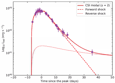
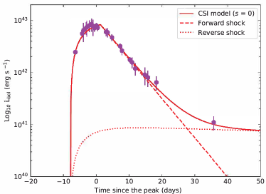
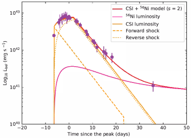
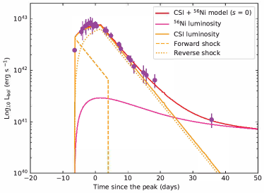
Figure 10: Best-fit light curves of SN 2019uo fitted with a CSI model and a combination of ⁵⁶Ni and CSI. The forward shocks, reverse shocks, and ⁵⁶Ni models are plotted with different lines.

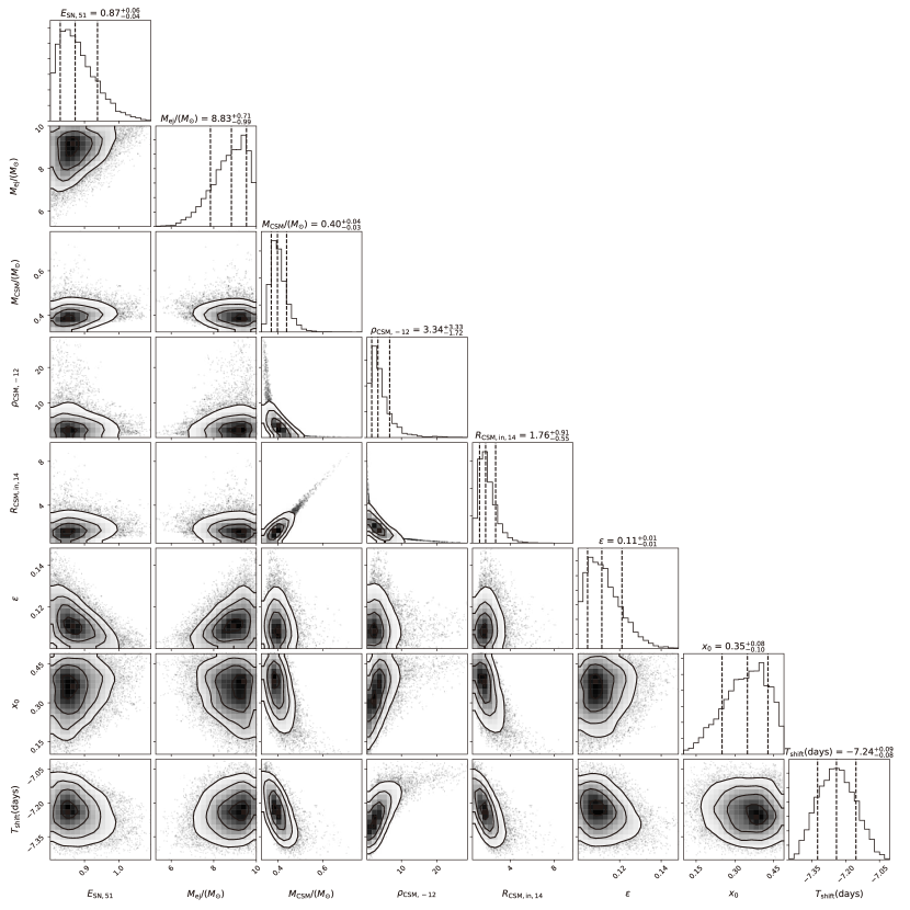
Figure 11: The corner plot of the CSI wind model displaying covariance of estimated parameters.

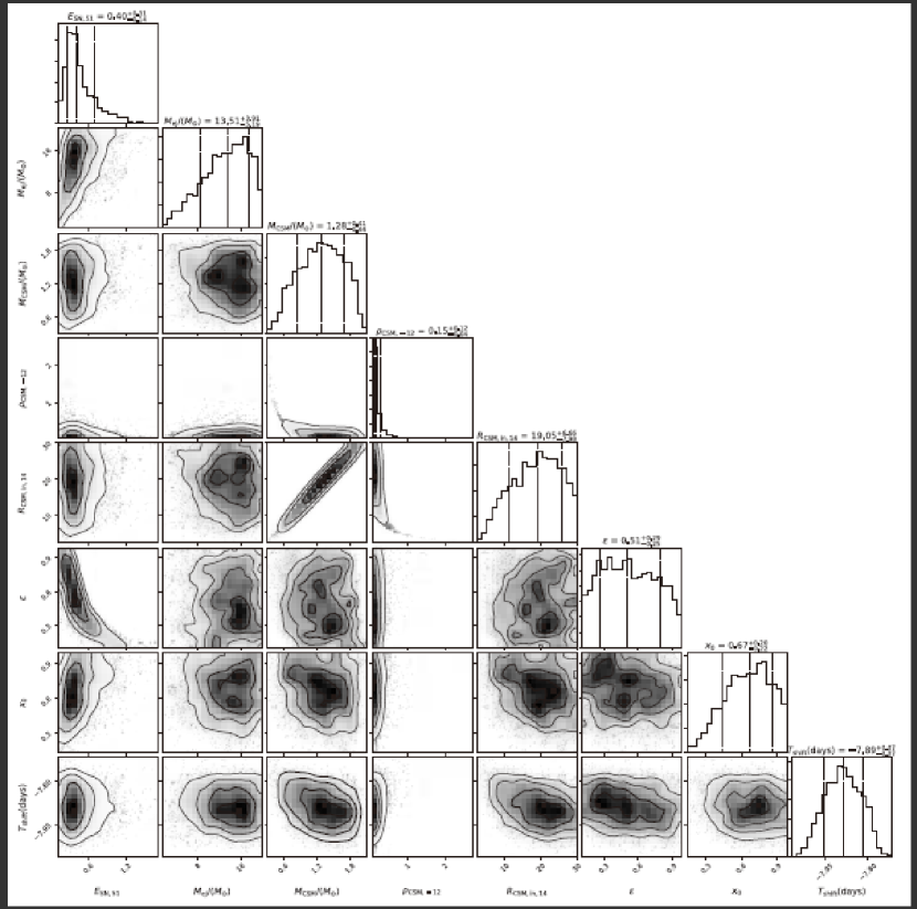
Figure 12: The corner plot of the CSI shell model displaying covariance of estimated parameters.

Figure 13: The corner plot of the ⁵⁶Ni + CSI wind model displaying covariance of estimated parameters.

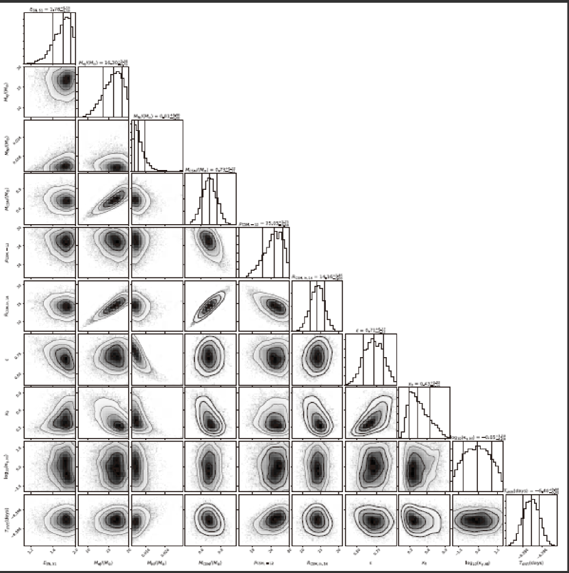
Figure 14: The corner plot of the ⁵⁶Ni + CSI shell model displaying covariance of estimated parameters.

The CSI model and the ⁵⁶Ni + CSI model: The narrow He emission lines appearing in the spectra of SN 2019uo indicate a potential source of circumstellar interaction (CSI) with a nearby He-rich shell. Thus, the nearby He-rich wind or shell surrounding the progenitor could be the essential powering source of the bolometric light curve of SN 2019uo. We take into account the ejecta-CSM interaction model (i.e., the CSI model) (Chevalier, 1982; Chevalier & Fransson, 1994; Chugai & Danziger, 1994; Ginzburg & Balberg, 2012; Liu et al., 2018) and the ⁵⁶Ni + CSI model (Chatzopoulos et al., 2012). To fit the bolometric light curve of SN 2019uo, we adopt the formulation given in Wang & Li (2019).

The ejecta can be broadly distinguished into two zones, the inner part ($\rho_{\mathrm{ej}}\propto r^{-\delta}$) and the outer part ($\rho_{\mathrm{ej}}\propto r^{-n}$). The density profile of the CSM can typically be described as a power law where $\rho_{\mathrm{CSM}}\propto r^{-s}$, where $s=0$ corresponds to shells of the CSM and $s=2$ corresponds to winds. Assuming $\delta=1$ and $n=10$, the adopted parameters of the CSM model are the energy of the SN ($E_{\mathrm{SN}}$), the mass of the ejecta ($M_{\mathrm{ej}}$), the mass of the CSM ($M_{\mathrm{CSM}}$), the density of the innermost part of the CSM $\rho_{\mathrm{CSM,in}}$, the radius of the innermost part of the ejecta $R_{\mathrm{CSM,in}}$, the efficiency factor which converts kinetic energy to radiation ($\epsilon$), the dimensionless $x_{0}$ parameter, and t_expl. Two additional parameters are used in the ⁵⁶Ni + CSI model, $M_{\mathrm{Ni}}$ and $\kappa_{\gamma,\mathrm{Ni}}$. The best-fit parameters of the model are tabulated in Table 4 and the best-fit models are displayed in Fig. 10. The corner plots describing covariance of the parameters are shown in Fig. 11, Fig. 12, Fig. 13 and Fig. 14 respectively. The tabulated values of ejecta masses of the four models are reasonable if the progenitor is a WR star of mass $\sim\!25\ M_{\odot}$ and the metallicity is nearly solar (Crowther & Smartt, 2007). We adopted the ⁵⁶Ni, CSI model, and the ⁵⁶Ni + CSI models to fit the bolometric light curve of SN 2019uo. The ⁵⁶Ni model provides a favourable fit to the light curve, but this model cannot explain the He I emission lines present in the spectrum of SN 2019uo. These lines are likely generated because of the CSI. We therefore invoke CSI as the more favourable model to model light curve. For the CSI model, the estimated ejecta masses for $s=0$ and $s=2$ are $8.83^{+0.71}_{-0.99}\ M_{\odot}$ and $13.51^{+3.91}_{-5.19}\ M_{\odot}$ respectively. This model, however, did not take into account the role of ⁵⁶Ni. Using the combination of both ⁵⁶Ni + CSI, the estimated $M_{\mathrm{ej}}$ for $s=0$ and $s=2$ is $15.99^{+2.25}_{-2.98}\ M_{\odot}$ and $16.30^{+2.09}_{-2.72}\ M_{\odot}$, respectively, which are consistent with a WR progenitor scenario. The mass-loss rate is given by $\dot{M}=4\pi v_{\mathrm{w}}q$ (where $q=\rho_{\mathrm{CSM,in}}R_{\mathrm{CSM,in}}^{2}$). The velocity of the wind v_w = 100-1000 km s^-1 for WR systems. Considering the wind CSI model (s = 2), we find that the estimated mass-loss rate lies between 0.195-1.95 $M_{\odot}$ yr^-1, which is comparable with the values obtained for iPTF13z (0.1–2 $M_{\odot}$ yr^-1; Nyholm et al., 2017) and PS15dpn (1–10 $M_{\odot}$ yr^-1; Wang & Li, 2019). Using the combination of ⁵⁶Ni + CSI model (s = 2), the estimated mass loss rate lies between 25.5-255.4 $M_{\odot}$ yr^-1 which is significantly higher than the value obtained for iPTF13z, PS15dpn, and this model can be excluded. Neverthless, the ⁵⁶Ni+CSM shell is reasonable.

For the CSM shell and the ⁵⁶Ni + CSM shell model, the expelled shell mass prior to explosion are $\sim$1.3 $M_{\odot}$ and 0.73 M_⊙, respectively. The radius of the inner shell for the ⁵⁶Ni + CSI model, as seen from Table 4, is $14\times 10^{14}$ cm and the typical velocity of WR winds is between 100 and 1000 km s^-1 ($10^{7-8}$ cm s^-1); so the time at which the shell is expelled prior to explosion is estimated to be between $1.4\times 10^{6}$ s and $1.4\times 10^{7}$ s, i.e., between 163.8 and 1638.8 days.

6 Summary

In this paper, we present the photometric and spectral evolution of the type Ibn SN 2019uo. The typical light curve decay rate of SNe Ibn is $\sim$0.1 mag d^-1 in all bands which is in agreement with the decline rates of the SNe Ibn discussed by Hosseinzadeh et al. (2017). The color evolution of SN 2019uo is similar to SN 2010al and iPTF14aki which places it between SNe Ib and SNe Ibn. This is in good agreement with the P Cygni spectroscopic features that transition from narrow to broad, indicating a He-rich circumstellar shell around the progenitor star along with optically thick CSM (Hosseinzadeh et al., 2017). The absolute magnitude ($M^{V}_{max}$ = $-$18.30 $\pm$ 0.24 mag) indicates that SN 2019uo lies at the fainter end of the group. We fit the bolometric light curve of SN 2019uo with ⁵⁶Ni model. However, the ⁵⁶Ni model alone does not take into account the CSM interaction that is evident from the narrow emission lines in the spectra of SN 2019uo. Thus, we also fit the light curves with a CSI model and a ⁵⁶Ni + CSI model. The ⁵⁶Ni + CSI wind (s=2) model can be excluded since an unrealistic value of mass loss rate (25.5-255.4 $M_{\odot}$ yr^-1) is required and the ⁵⁶Ni + CSI shell model is reasonable. The combination of ⁵⁶Ni + CSI shell well fits our observed light curve, with ejecta masses consistent with a WR star. The spectroscopic features of SN 2019uo indicate that it is the second SNe Ibn with flash ionization signatures. Prominent lines of He II, C III, and N III are detected in the spectra, similar to SN 2010al. SN 2019uo shows initial P Cygni He I features that broadens after 11 days post-maximum. This can originate from a He-rich shell around progenitor surrounded by dense CSM, or it may be due to viewing angle dependency. This is also validated by the equivalent widths of He I features. Alternatively, P-cygni spectroscopic features usually originate from optical depths $\leq$ 1. As X-rays penetrate into the P-cygni producing regions absorptions are filled leading to subsequent emission features. The estimated line velocities are lower than the average SN Ibn, but they show a faster evolution compared to the group of SNe that show prominent emission features from the beginning.

References

- Andrews & Smith (2018) Andrews, J. E., & Smith, N. 2018, MNRAS, 477, 74, doi: 10.1093/mnras/sty584
- Arnett (1980) Arnett, W. D. 1980, ApJ, 237, 541, doi: 10.1086/157898
- Arnett (1982) —. 1982, ApJ, 253, 785, doi: 10.1086/159681
- Becker (2015) Becker, A. 2015, HOTPANTS: High Order Transform of PSF ANd Template Subtraction. http://ascl.net/1504.004
- Chatzopoulos et al. (2012) Chatzopoulos, E., Wheeler, J. C., & Vinko, J. 2012, ApJ, 746, 121, doi: 10.1088/0004-637X/746/2/121
- Chevalier (1982) Chevalier, R. A. 1982, ApJ, 258, 790, doi: 10.1086/160126
- Chevalier & Fransson (1994) Chevalier, R. A., & Fransson, C. 1994, ApJ, 420, 268, doi: 10.1086/173557
- Chugai & Danziger (1994) Chugai, N. N., & Danziger, I. J. 1994, MNRAS, 268, 173, doi: 10.1093/mnras/268.1.173
- Cooke et al. (2010) Cooke, J., Ellis, R. S., Nugent, P. E., et al. 2010, The Astronomer’s Telegram, 2491, 1
- Crowther & Smartt (2007) Crowther, P., & Smartt, S. 2007, Astronomy and Geophysics, 48, 1.35, doi: 10.1111/j.1468-4004.2007.48135.x
- Fassia et al. (2001) Fassia, A., Meikle, W. P. S., Chugai, N., et al. 2001, MNRAS, 325, 907, doi: 10.1046/j.1365-8711.2001.04282.x
- Foley et al. (2007) Foley, R. J., Smith, N., Ganeshalingam, M., et al. 2007, ApJ, 657, L105, doi: 10.1086/513145
- Fremling et al. (2019) Fremling, C., Dugas, A., & Sharma, Y. 2019, Transient Name Server Classification Report, 2019-188, 1
- Gal-Yam (2014) Gal-Yam, A. 2014, in American Astronomical Society Meeting Abstracts, Vol. 223, American Astronomical Society Meeting Abstracts #223, 235.02
- Gal-Yam et al. (2014) Gal-Yam, A., Arcavi, I., Ofek, E. O., et al. 2014, Nature, 509, 471, doi: 10.1038/nature13304
- Ginzburg & Balberg (2012) Ginzburg, S., & Balberg, S. 2012, ApJ, 757, 178, doi: 10.1088/0004-637X/757/2/178
- Gorbikov et al. (2014) Gorbikov, E., Gal-Yam, A., Ofek, E. O., et al. 2014, MNRAS, 443, 671, doi: 10.1093/mnras/stu1184
- Hakobyan et al. (2012) Hakobyan, A. A., Adibekyan, V. Z., Aramyan, L. S., et al. 2012, A&A, 544, A81, doi: 10.1051/0004-6361/201219541
- Hosseinzadeh et al. (2019) Hosseinzadeh, G., McCully, C., Zabludoff, A. I., et al. 2019, ApJ, 871, L9, doi: 10.3847/2041-8213/aafc61
- Hosseinzadeh et al. (2017) Hosseinzadeh, G., Arcavi, I., Valenti, S., et al. 2017, ApJ, 836, 158, doi: 10.3847/1538-4357/836/2/158
- Jordi et al. (2006) Jordi, K., Grebel, E. K., & Ammon, K. 2006, A&A, 460, 339, doi: 10.1051/0004-6361:20066082
- Karamehmetoglu et al. (2019) Karamehmetoglu, E., Fransson, C., Sollerman, J., et al. 2019, arXiv e-prints, arXiv:1910.06016. https://arxiv.org/abs/1910.06016
- Khazov et al. (2016) Khazov, D., Yaron, O., Gal-Yam, A., et al. 2016, ApJ, 818, 3, doi: 10.3847/0004-637X/818/1/3
- Liu et al. (2018) Liu, L.-D., Wang, L.-J., Wang, S.-Q., & Dai, Z.-G. 2018, ApJ, 856, 59, doi: 10.3847/1538-4357/aab157
- Lusk & Baron (2017) Lusk, J. A., & Baron, E. 2017, PASP, 129, 044202, doi: 10.1088/1538-3873/aa5e49
- Lyman et al. (2016) Lyman, J. D., Bersier, D., James, P. A., et al. 2016, MNRAS, 457, 328, doi: 10.1093/mnras/stv2983
- Morozova et al. (2017) Morozova, V., Piro, A. L., & Valenti, S. 2017, ApJ, 838, 28, doi: 10.3847/1538-4357/aa6251
- Munari & Zwitter (1997) Munari, U., & Zwitter, T. 1997, A&A, 318, 269
- Nicholl (2018) Nicholl, M. 2018, Research Notes of the American Astronomical Society, 2, 230, doi: 10.3847/2515-5172/aaf799
- Nyholm et al. (2017) Nyholm, A., Sollerman, J., Taddia, F., et al. 2017, A&A, 605, A6, doi: 10.1051/0004-6361/201629906
- Pastorello et al. (2007) Pastorello, A., Smartt, S. J., Mattila, S., et al. 2007, Nature, 447, 829, doi: 10.1038/nature05825
- Pastorello et al. (2008) Pastorello, A., Mattila, S., Zampieri, L., et al. 2008, MNRAS, 389, 113, doi: 10.1111/j.1365-2966.2008.13602.x
- Pastorello et al. (2015a) Pastorello, A., Wyrzykowski, Ł., Valenti, S., et al. 2015a, MNRAS, 449, 1941, doi: 10.1093/mnras/stu2621
- Pastorello et al. (2015b) Pastorello, A., Hadjiyska, E., Rabinowitz, D., et al. 2015b, MNRAS, 449, 1954, doi: 10.1093/mnras/stv335
- Pastorello et al. (2015c) Pastorello, A., Benetti, S., Brown, P. J., et al. 2015c, MNRAS, 449, 1921, doi: 10.1093/mnras/stu2745
- Pastorello et al. (2015d) Pastorello, A., Prieto, J. L., Elias-Rosa, N., et al. 2015d, MNRAS, 453, 3649, doi: 10.1093/mnras/stv1812
- Pastorello et al. (2016) Pastorello, A., Wang, X. F., Ciabattari, F., et al. 2016, MNRAS, 456, 853, doi: 10.1093/mnras/stv2634
- Poznanski et al. (2012) Poznanski, D., Prochaska, J. X., & Bloom, J. S. 2012, MNRAS, 426, 1465, doi: 10.1111/j.1365-2966.2012.21796.x
- Prentice et al. (2016) Prentice, S. J., Mazzali, P. A., Pian, E., et al. 2016, MNRAS, 458, 2973, doi: 10.1093/mnras/stw299
- Prentice et al. (2019) Prentice, S. J., Ashall, C., James, P. A., et al. 2019, MNRAS, 485, 1559, doi: 10.1093/mnras/sty3399
- Sanders et al. (2013) Sanders, N. E., Soderberg, A. M., Foley, R. J., et al. 2013, ApJ, 769, 39, doi: 10.1088/0004-637X/769/1/39
- Schlafly & Finkbeiner (2011) Schlafly, E. F., & Finkbeiner, D. P. 2011, ApJ, 737, 103, doi: 10.1088/0004-637X/737/2/103
- Schlegel (1990) Schlegel, E. M. 1990, MNRAS, 244, 269
- Shivvers et al. (2016) Shivvers, I., Zheng, W. K., Mauerhan, J., et al. 2016, MNRAS, 461, 3057, doi: 10.1093/mnras/stw1528
- Silverman et al. (2010) Silverman, J. M., Kleiser, I. K. W., Morton, A. J. L., & Filippenko, A. V. 2010, Central Bureau Electronic Telegrams, 2223, 1
- Smith et al. (2008) Smith, N., Foley, R. J., & Filippenko, A. V. 2008, ApJ, 680, 568, doi: 10.1086/587860
- Stetson (1987) Stetson, P. B. 1987, PASP, 99, 191, doi: 10.1086/131977
- Sun et al. (2019) Sun, N.-C., Maund, J. R., Hirai, R., Crowther, P. A., & Podsiadlowski, P. 2019, arXiv e-prints, arXiv:1909.07999. https://arxiv.org/abs/1909.07999
- Taddia et al. (2013) Taddia, F., Stritzinger, M. D., Sollerman, J., et al. 2013, A&A, 555, A10, doi: 10.1051/0004-6361/201321180
- Tody (1986) Tody, D. 1986, Society of Photo-Optical Instrumentation Engineers (SPIE) Conference Series, Vol. 627, The IRAF Data Reduction and Analysis System, ed. D. L. Crawford, 733, doi: 10.1117/12.968154
- Tody (1993) —. 1993, Astronomical Society of the Pacific Conference Series, Vol. 52, IRAF in the Nineties, ed. R. J. Hanisch, R. J. V. Brissenden, & J. Barnes, 173
- Valenti et al. (2011) Valenti, S., Fraser, M., Benetti, S., et al. 2011, MNRAS, 416, 3138, doi: 10.1111/j.1365-2966.2011.19262.x
- Valenti et al. (2014) Valenti, S., Sand, D., Pastorello, A., et al. 2014, MNRAS, 438, L101, doi: 10.1093/mnrasl/slt171
- Valenti et al. (2016) Valenti, S., Howell, D. A., Stritzinger, M. D., et al. 2016, MNRAS, 459, 3939, doi: 10.1093/mnras/stw870
- Wang & Li (2019) Wang, S.-Q., & Li, L. 2019, arXiv e-prints, arXiv:1905.12623. https://arxiv.org/abs/1905.12623
- Zhang et al. (2019) Zhang, J., Xing, L., & Wang, X. 2019, The Astronomer’s Telegram, 12410