Robust Adaptive Least Squares Polynomial Chaos Expansions in High-Frequency Applications

Abstract

We present an algorithm for computing sparse, least squares-based polynomial chaos expansions, incorporating both adaptive polynomial bases and sequential experimental designs. The algorithm is employed to approximate stochastic high-frequency electromagnetic models in a black-box way, in particular, given only a dataset of random parameter realizations and the corresponding observations regarding a quantity of interest, typically a scattering parameter. The construction of the polynomial basis is based on a greedy, adaptive, sensitivity-related method. The sequential expansion of the experimental design employs different optimality criteria, with respect to the algebraic form of the least squares problem. We investigate how different conditions affect the robustness of the derived surrogate models, that is, how much the approximation accuracy varies given different experimental designs. It is found that relatively optimistic criteria perform on average better than stricter ones, yielding superior approximation accuracies for equal dataset sizes. However, the results of strict criteria are significantly more robust, as reduced variations regarding the approximation accuracy are obtained, over a range of experimental designs. Two criteria are proposed for a good accuracy-robustness trade-off.

keywords— polynomial chaos, surrogate modeling, high-frequency electromagnetic devices, least squares regression, adaptive basis, sequential experimental design

1 Introduction

For most, if not all, electromagnetic (EM) devices, quantities of interest (QoIs) feature a parametric dependency upon the design characteristics of the device, e.g., its geometry or material properties. During the design of an EM device, this dependency, denoted here with $g(\mathbf{y})$, where $\mathbf{y}\in\mathbb{R}^{N}$ is the parameter vector, is typically resolved with a computationally expensive parametric simulation, e.g., using a finite element (FE) model. In this work, our goal is to infer (learn, approximate) the relation between the design parameters of a high-frequency EM device and its QoIs, e.g., one or more scattering parameters, and compute a black-box approximation $\widetilde{g}\approx g$, given only a dataset $\mathcal{D}=\left\{\mathbf{y}_{l},g(\mathbf{y}_{l})\right\}_{l=1}^{L}$. This approximation is often called a surrogate model, a meta-model, or a response surface. We call the set of parameter realizations $\left\{\mathbf{y}_{l}\right\}_{l=1}^{L}$ the experimental design (ED) and the corresponding QoI values $\left\{g(\mathbf{y}_{l})\right\}_{l=1}^{L}$ the observations. The latter shall here be simulation outputs, however, they could also refer to - possibly noisy - measurement data as well.

The aforementioned inference problem is here considered in an uncertainty quantification (UQ) setting [54, 57]. In particular, the model parameters are assumed to be independent random variables (RVs) $Y_{n}$, $n=1,\dots,N$, forming the $N$-variate RV $\mathbf{Y}=\left(Y_{1},\dots,Y_{N}\right)$. The latter is defined on the probability space $\left(\Theta,\Sigma,P\right)$ and follows the probability density function (PDF) $\varrho:\Xi\rightarrow\mathbb{R}_{\geq 0}$, where $\Xi$ denotes the image space. Due to the RV independence, it holds that $\varrho(\mathbf{y})=\prod_{n=1}^{N}\varrho_{n}(y_{n})$, where $\mathbf{y}=\mathbf{Y}\left(\theta\right)\in\Xi$, $\theta\in\Theta$, is now a RV realization. We note that RV independence is not a crucial assumption and that dependencies can also be handled via suitable RV transformations [20, 34, 38]. The RVs represent here random deviations from the specifications of a high-frequency device, which may arise due to manufacturing tolerances, material contamination, or other uncertainty sources.

Assuming that $g$ corresponds to a smooth functional relation, a computationally efficient approach for constructing a surrogate model is to compute a polynomial chaos expansion (PCE) [23, 61]

$$\widetilde{g}(\mathbf{y})=\sum_{m=1}^{M}s_{m}\Psi_{m}(\mathbf{y}),$$ (1)

where $s_{m}$ are scalar coefficients and $\Psi_{m}$ are polynomials orthogonal to the input PDF. Once available, the PCE can replace the original model in computationally demanding tasks, e.g., UQ or optimization studies. For the purposes of UQ, certain statistical measures regarding the QoI can be computed by simply post-processing the PCE’s terms [8, 56]. Moreover, the corresponding computational cost is typically orders of magnitude smaller than the one of a Monte Carlo (MC) method [11, 39]. In this work, given a dataset $\mathcal{D}$ of size $L$, the PCE is constructed by solving the discrete least squares (LS) minimization problem

$$\widetilde{g}=\operatorname*{arg\,min}_{\pi\in\mathbb{P}_{M}}\sum_{l=1}^{L}\left(g\left(\mathbf{y}_{l}\right)-\pi\left(\mathbf{y}_{l}\right)\right)^{2},$$ (2)

where $\mathbb{P}_{M}=\text{span}\left\{\Psi_{m},m=1,\dots,M\right\}$ denotes the corresponding polynomial space [12, 45, 46]. Note that the surrogate model is constructed in a non-intrusive way, i.e., the model is used as a black box to compute the observations $g(\mathbf{y}_{l})$, $l=1,\dots,L$. The construction of the PCE can alternatively be based on compressive sensing [16, 17, 29, 32, 50] or low-rank tensor decomposition methods [18, 36, 35]. Nevertheless, many recent works on both the theoretical properties of LS methods [12, 13, 15, 45, 46, 44, 43] and on LS-PCE algorithms [7, 8, 9, 10, 19, 27, 42] indicate that the interest in this approach remains active. In the context of this work, a further reason for investigating and improving the LS-PCE method is its popularity in the setting of EM simulations [24, 31, 47, 48, 52].

The approximation accuracy of the PCE is crucially affected by the choice of the polynomial space $\mathbb{P}_{M}$. This is especially relevant in high-dimensional approximations, due to the fact that the dimension of $\mathbb{P}_{M}$ grows very fast with the number of RVs, which constitutes a manifestation of the so-called curse of dimensionality [6]. To mitigate this problem, a sparse albeit expressive polynomial basis must be constructed [7, 9, 15, 17, 32, 42, 50]. The first contribution of this work is exactly in this direction. Specifically, we propose a greedy-adaptive algorithm for the construction of the PCE basis, which takes into consideration the sensitivity of the QoI to the input RVs and the corresponding PCE terms.

Another crucial aspect regarding the stability of the LS problem (2) and the accuracy of its solution is the relation between the size of the polynomial basis and the size of the ED, equivalently, of the dataset [12, 13, 46]. At minimum, the LS system must not be underdetermined, i.e., it must hold that $L\geq M$. Consequently, considering an adaptively constructed PCE basis, the ED must be sequentially expanded in order to meet the stability requirements. Theoretical LS stability criteria have been established in the literature [12, 13, 46, 44] and have been used to form sequential ED strategies [15, 42]. However, it has been observed that relaxed criteria typically result in more accurate approximations for equal costs [12, 45, 42, 46, 43]. Therefore, most works resort to heuristic criteria regarding the dynamic relation between the polynomial basis and the dataset [7, 9]. In the same vein, optimal ED criteria have been considered recently [10, 16, 19, 27]. In this case, optimality refers to selecting the best available realizations over a pool of candidate realizations to enhance the ED.

Mostly, the aforementioned works focus on the accuracy of the PCEs derived with the proposed heuristic conditions regarding sequential EDs. However, studies on the robustness of the approximation, i.e., to what extent different EDs affect the accuracy of a surrogate model constructed with a specific method or adaptivity criterion, have not been sufficiently addressed in the literature so far. There lies the second contribution of this work, which aims to address the issue of robustness. Specifically, we examine different optimality conditions during the sequential expansion of the ED and their impact on both the accuracy and the robustness of the resulting PCEs. In combination with the proposed greedy-adaptive polynomial basis, a fully adaptive PCE algorithm is developed, where both the polynomial basis and the ED are sequentially/adaptively expanded.

Our method is tested on two simulation models from the field of high-frequency electromagnetics. First, an academic test case is considered, employing a simple rectangular waveguide with dielectric filling [41, 40] and featuring up to $15$ parameters. Second, we apply the method to an optical grating coupler model [51] with up to $5$ parameters. By including the frequency in the parameter vector, we are able to approximate not only the parametric dependence, but also the frequency response of the model, within a given frequency range. Naturally, the frequency response must also correspond to a smooth functional, e.g., sharp resonances shall increase the computational cost of the method, or might even render it inapplicable altogether. For both considered numerical examples, the suggested approach results in accurate surrogate models for comparably low dataset sizes. We observe the influence of the different optimality criteria upon the accuracy and the robustness of the PCEs. On the one hand, relaxed criteria result in - on average - more accurate surrogate models, which however vary significantly from one another for different EDs. On the other hand, stricter criteria yield approximations of inferior accuracy, however, the variance of the approximation accuracy for different EDs is significantly reduced. Two sequential ED criteria are identified, for which the trade-off between accuracy and robustness can be considered as acceptable.

The rest of this paper is organized as follows. In Section 2 we introduce the PCE as well as the computation of the corresponding coefficients via discrete LS. This is followed by Section 3 where we present a scheme which exploits the sensitivity of the QoI on the RVs for adaptively selecting the PCE basis terms. In the same section, we extend the scheme by robust sequential ED, relying on different optimality criteria. Numerical experiments on two high-frequency electromagnetic devices verify the reliability and accuracy of the presented method in Section 4. Concluding remarks and possible continuations of this work are available in Section 5.

2 Least Squares Polynomial Chaos Expansions

2.1 Univariate Polynomial Chaos Expansions

We first consider a univariate model $g(y)$, where $y=Y\left(\theta\right)$, $\theta\in\Theta$, and the RV $Y$ is characterized by the PDF $\varrho(y)$. We denote a univariate polynomial of degree $p\in\mathbb{Z}_{\geq 0}$ with $\psi_{p}$ and demand that the polynomial basis $\left\{\psi_{p}\right\}_{p=0}^{p_{\text{max}}}$ is orthogonal with respect to the univariate PDF, such that

$$\mathbb{E}\left[\psi_{p}\psi_{q}\right]=\int_{\Xi}\psi_{p}(y)\psi_{q}(y)\varrho(y)\,\mathrm{d}y=\gamma_{p}\delta_{p,q},$$ (3)

where $p,q\in\left\{0,1,\dots,p_{\text{max}}\right\}$, $\delta_{p,q}$ is the Kronecker delta, and $\gamma_{p}$ a normalization factor. In the rest of this paper, we will always assume that $\gamma_{p}=1$, $\forall p\in\left\{0,1,\dots,p_{\text{max}}\right\}$, i.e., that $\left\{\psi_{p}\right\}_{p=0}^{p_{\text{max}}}$ is an orthonormal basis. For commonly used PDFs, the generalized polynomial chaos (gPC) or Wiener-Askey scheme [61] provides correspondences to families of orthogonal polynomials. Extensions to arbitrary PDFs have been introduced by using numerically constructed orthogonal polynomials [49, 55, 60]. The univariate PCE reads

$$g(y)\approx\widetilde{g}(y)=\sum_{p=0}^{p_{\max}}s_{p}\psi_{p}(y),$$ (4)

where $s_{p}\in\mathbb{R}$ are scalar coefficients. In essence, $\widetilde{g}$ is a polynomial living in the space

$$\mathbb{P}_{p_{\text{max}}}=\text{span}\left\{\psi_{p}:p\leq p_{\text{max}}\right\}.$$ (5)

2.2 Multivariate Polynomial Chaos Expansions

We proceed to the case of a multivariate model $g(\mathbf{y})$, where $\mathbf{y}=\mathbf{Y}\left(\theta\right)$ and the RVs $\mathbf{Y}$ are characterized by the PDF $\varrho(\mathbf{y})=\varrho_{1}(y_{1})\cdots\varrho_{N}(y_{N})$. We introduce the multi-index $\mathbf{p}=\left(p_{1},\dots,p_{N}\right)\in\mathbb{Z}_{\geq 0}^{N}$ which contains the polynomial order per parameter and defines the corresponding multivariate polynomial $\Psi_{\mathbf{p}}$ as

$$\Psi_{\mathbf{p}}(\mathbf{y})=\prod_{n=1}^{N}\psi_{p_{n}}(y_{n}).$$ (6)

In this case, the orthonormality condition reads

$$\mathbb{E}\left[\Psi_{\mathbf{p}}\Psi_{\mathbf{q}}\right]=\int_{\Xi}\Psi_{\mathbf{p}}\left(\mathbf{y}\right)\Psi_{\mathbf{q}}\left(\mathbf{y}\right)\varrho\left(\mathbf{y}\right)\mathrm{d}\mathbf{y}=\delta_{\mathbf{p}\mathbf{q}},$$ (7)

where $\delta_{\mathbf{p}\mathbf{q}}=\delta_{p_{1}q_{1}}\cdots\delta_{p_{N}q_{N}}$. Assuming a polynomial basis $\left\{\Psi_{\mathbf{p}}\right\}_{\mathbf{p}\in\Lambda}$, where $\Lambda$ is a multi-index set, the multivariate PCE reads

$$g\left(\mathbf{y}\right)\approx\widetilde{g}\left(\mathbf{y}\right)=\sum_{\mathbf{p}:\mathbf{p}\in\Lambda}s_{\mathbf{p}}\Psi_{\mathbf{p}}\left(\mathbf{y}\right),$$ (8)

and the corresponding multivariate polynomial space $\mathbb{P}_{\Lambda}$ is given by

$$\mathbb{P}_{\Lambda}=\text{span}\left\{\Psi_{\mathbf{p}}:\mathbf{p}\in\Lambda\right\}.$$ (9)

Common choices for $\Lambda$ in the literature are tensor product (TP), total degree (TD), hyperbolic cross (HC), and downward-closed (DC) multi-index sets [4, 12, 46]. The respective definitions are given in Table 1, where $\mathbf{e}_{n}$ denotes the $n$-th unit vector. We note that multi-index sets of arbitrary shapes may also be used, see, e.g., [7, 8].

Table 1: Definitions of commonly employed multi-index sets, respectively, polynomial bases.

TP	$\Lambda^{\mathrm{TP}}\coloneqq\left\{\mathbf{p}:\max_{n}(p_{n})\leq p^{\max},p^{\max}\in\mathbb{Z}_{\geq 0}\right\}$
TD	$\Lambda^{\mathrm{TD}}\coloneqq\left\{\mathbf{p}:\sum_{n=1}^{N}p_{n}\leq p^{\max},p^{\max}\in\mathbb{Z}_{\geq 0}\right\}$
HC	$\Lambda^{\mathrm{HC}}\coloneqq\left\{\mathbf{p}:\prod_{n=1}^{N}\left(p_{n}+1\right)\leq p^{\max}+1,p^{\max}\in\mathbb{Z}_{\geq 0}\right\}$
DC	$\Lambda^{\mathrm{DC}}\coloneqq\left\{\mathbf{p}:\left(\mathbf{p}-\mathbf{e}_{n}\right)\in\Lambda^{\mathrm{DC}},\forall n=1,\dots,N\>\text{with}\>p_{n}>0\right\}$

2.3 Computing Expansion Coefficients via Discrete Least Squares

We now assume that a polynomial basis $\left\{\Psi_{\mathbf{p}}\right\}_{\mathbf{p}\in\Lambda}$ with cardinality $\#\Lambda=M$, as well as an ED $\left\{\mathbf{y}_{l}\right\}_{l=1}^{L}$ and the corresponding observations $\left\{g\left(\mathbf{y}_{l}\right)\right\}_{l=1}^{L}$, are available. Then, the PCE can be obtained by solving the minimization problem (2), where the polynomial space is defined as in (9). For the solution of (2), we introduce the design matrix $\mathbf{D}\in\mathbb{R}^{L\times M}$ with elements $d_{lm}=\Psi_{m}\left(\mathbf{y}_{l}\right)$, and the observation vector $\mathbf{b}=\left(g(\mathbf{y}_{1}),\dots,g(\mathbf{y}_{L})\right)^{\top}$. Collecting the unknown PCE coefficients into a vector $\mathbf{s}=\left(s_{1},\dots,s_{M}\right)^{\top}$, we form the discrete minimization problem

$$\mathbf{s}=\operatorname*{arg\,min}_{\hat{\mathbf{s}}\in\mathbb{R}^{M}}\|\mathbf{D}\hat{\mathbf{s}}-\mathbf{b}\|_{2}.$$ (10)

Applying the necessary conditions for a minimum, we obtain the normal equation [30, Section 20.4]

$$\left(\mathbf{D}^{\top}\mathbf{D}\right)\mathbf{s}=\mathbf{D}^{\top}\mathbf{b},$$ (11)

where the system matrix $\mathbf{A}=\mathbf{D}^{\top}\mathbf{D}$ is called the information matrix. The solution to (11) is unique if the design matrix is nonsingular. Moreover, it must obviously hold that $L\geq M$, i.e., the system of equations cannot be underdetermined.

Due to the well-known estimates regarding the sensitivity of the LS solution and its dependence on the condition number $\kappa\left(\cdot\right)$ of the corresponding system matrix [25, 30], it is generally not recommended to use the normal equation (11), as it can easily be shown that

$$\kappa\left(\mathbf{A}\right)=\left(\kappa\left(\mathbf{D}\right)\right)^{2}.$$ (12)

A QR decomposition of the design matrix $\mathbf{D}$ can be used instead [30, Section 20.2], in which case the conditioning of the LS system is given by $\kappa\left(\mathbf{D}\right)=\kappa\left(\mathbf{Q}\mathbf{R}\right)=\kappa\left(\mathbf{R}\right)$.

3 Adaptive Least Squares Polynomial Approximations

3.1 Adaptive Polynomial Basis

We first address the case of a fixed dataset $\mathcal{D}=\left\{\mathbf{y}_{l},b_{l}\right\}_{l=1}^{L}$, which is considered to be sufficient for computing a PCE with $M$ terms. The question which arises is, which $M$ polynomials, equivalently, which multi-index set $\Lambda$ with $\#\Lambda=M$ will result in an accurate approximation. Several algorithms have been developed to address this problem [7, 8, 9, 17, 32, 27, 28, 42, 50]. Any of these approaches can be combined with the sequential ED strategies discussed in Section 3.2.

Additionally to the aforementioned methods, we present here yet another algorithm for the adaptive construction of the PCE basis. Our approach is conceptually similar to a well-known dimension-adaptive quadrature method [22], therefore, we enforce the use of DC multi-index sets, as defined in Table 1. We note that DC sets are not strictly necessary. For example, the simple two-dimensional function

$$g\left(y_{1},y_{2}\right)=ay_{1}^{2}+by_{2},$$ (13)

can be represented exactly by a PCE based on $\Lambda=\left\{\left(2,0\right),\left(0,1\right)\right\}$. However, the DC property would require that $\Lambda=\left\{\left(0,0\right),\left(1,0\right),\left(2,0\right),\left(0,1\right)\right\}$, thus unnecessarily augmenting the LS system matrix. Nevertheless, while not optimal, DC sets are employed in several theoretical works [12, 14, 15, 42, 45, 46] due to the fact that the corresponding polynomial spaces satisfy a number of desirable properties, e.g., closure under differentiation for any variable, and invariance under a change of basis. Moreover, as also verified by the results in Section 4, PCEs based on DC sets perform very well in practice. This can be attributed to the fact that pathological cases such as (13) are rarely encountered in practical applications.

The adaptive construction of the PCE basis proceeds as follows. Let us assume that a multivariate approximation (8) based on a DC multi-index set $\Lambda$ is readily available. If not, we can initialize the procedure with $\Lambda=\left\{\left(0,0,\dots,0\right)\right\}$. We call “admissible neighbors” the indices which do not belong to $\Lambda$ and would satisfy the DC property if added to $\Lambda$. The corresponding admissible set is defined as

$$\Lambda^{\mathrm{adm}}\coloneqq\left\{\mathbf{p}\not\in\Lambda\,:\,\left(\mathbf{p}-\mathbf{e}_{n}\right)\subset\Lambda,\forall n=1,\dots,N\>\>\text{with}\>\>p_{n}>0\right\}.$$ (14)

Next, we construct the basis corresponding to the multi-index set $\Lambda^{\text{LS}}=\Lambda\cup\Lambda^{\mathrm{adm}}$ and solve the discrete LS minimization problem (10) for the coefficients $s_{\mathbf{p}}$, $\mathbf{p}\in\Lambda^{\text{LS}}$. Assuming that orthonormal polynomials are used, the value $s_{\mathbf{p}}^{2}$ is the equivalent of the partial variance due to the multi-index $\mathbf{p}$, thus, directly linked to the contribution of that multi-index to the total variance of the QoI [8, 56]. Since Sobol sensitivity indices are nothing more than fractions of partial variances over the total variance of the QoI, the value $s_{\mathbf{p}}^{2}$ can be interpreted as a sensitivity indicator regarding the multi-index $\mathbf{p}$. Therefore, we add to $\Lambda$ the admissible multi-index which corresponds to the maximum sensitivity indicator, such that

$$\Lambda\leftarrow\Lambda\cup\left\{\mathbf{p}^{*}\right\},\hskip 4.5pt\text{where}\hskip 4.5pt\mathbf{p}^{*}=\operatorname*{arg\,max}_{\mathbf{p}\in\Lambda^{\mathrm{adm}}}s_{\mathbf{p}}^{2}.$$ (15)

This procedure continues iteratively until $\#\Lambda=M$ basis terms are reached, as shown in Algorithm 1.

Data: dataset $\mathcal{D}$, maximum PCE terms $M$, initial DC multi-index set $\Lambda^{\text{init}}.$

Result: DC multi-index set $\Lambda$ with $\#\Lambda=M$, PCE basis $\left\{\Psi_{\mathbf{p}}\right\}_{\mathbf{p}\in\Lambda}$ and coefficients $\left\{s_{\mathbf{p}}\right\}_{\mathbf{p}\in\Lambda}$.

while $\#\Lambda<M$ do

    Create the extended multi-index set $\Lambda^{\text{LS}}=\Lambda\cup\Lambda^{\text{adm}}$.

    Solve the LS problem (10) using $\Lambda^{\text{LS}}$.

    Find the admissible multi-index corresponding to the largest sensitivity indicator, i.e., $\mathbf{p}^{*}=\operatorname*{arg\,max}_{\mathbf{p}\in\Lambda^{\mathrm{adm}}}s_{\mathbf{p}}^{2}$.

    Expand $\Lambda$ with $\mathbf{p}^{*}$, i.e., $\Lambda=\Lambda\cup\mathbf{p}^{*}$.

end while

Algorithm 1 Adaptive PCE basis construction.

3.2 Sequential Experimental Design

We now consider the case where the PCE is expanded adaptively until it reaches a desired accuracy $e$. This accuracy is typically estimated using a cross-validation (CV) error metric, e.g., the leave-one-out (LOO) [8, 9, 19] or the $\ell^{\infty}$ [45, 42, 46] CV error. In that case, the dataset $\mathcal{D}$, accordingly, the ED and the observations, should also be expanded, such that the LS problem remains stable and the accuracy of the PCE increases. Moreover, this expansion should be sequential, such that previously available observations can be re-used, thus restricting the computational cost to the simulations due to the new parameter realizations. Such an approach falls in the category of sequential EDs [3, 7, 8, 9, 19].

We will focus here on three such criteria. Denoting with $\mathbf{G}=L^{-1}\mathbf{A}$ the normalized information matrix, those criteria are, (i) the $K$-optimality criterion, which aims to minimize the condition number $\kappa\left(\mathbf{G}\right)$, (ii) the $A$-optimality criterion, which aims to minimize the trace $\mathrm{tr}\left(\mathbf{G}^{-1}\right)$, and (iii) the $E$-optimality criterion, which aims to minimize the maximum eigenvalue $\lambda_{\max}\left(\mathbf{G}^{-1}\right)$. We note that $\kappa\left(\mathbf{G}\right)=\kappa\left(\mathbf{A}\right)=\kappa\left(\mathbf{D}\right)^{2}$, therefore, the $K$-optimality criterion can be modified such that the design matrix $\mathbf{D}$ is used instead. Moreover, it can be easily shown that $\lambda_{\max}\left(\mathbf{G}^{-1}\right)=\left(\lambda_{\min}\left(\mathbf{G}\right)\right)^{-1}$, thus, we can avoid the possibly costly inversions. The inversion can also be avoided when the trace-based criterion is used, by exploiting the property $\mathrm{tr}\left(\mathbf{G}^{-1}\right)=\sum_{m=1}^{M}\left(\lambda_{m}\left(G\right)\right)^{-1}$, where $\lambda_{m}\left(G\right)$ denotes the $m$-th eigenvalue of matrix $\mathbf{G}$.

Contrary to the setting of optimal EDs, in this work we do not seek to minimize those measures. Instead, we investigate conditions which, if violated, trigger the expansion of the dataset, equivalently, of the ED and the observations. In essence, we enforce the values of $\kappa\left(\mathbf{D}\right)$, $\mathrm{tr}\left(\mathbf{G}^{-1}\right)$, $\lambda_{\max}\left(\mathbf{G}^{-1}\right)$ to be below some limit value. If this condition is satisfied, the PCE is adaptively expanded using the available ED, as in Section 3.1. Otherwise, the polynomial basis remains fixed and the dataset is expanded until the condition is again satisfied. This sequential ED strategy is depicted in Algorithm 2. Several works claim that relaxed conditions may lead to more accurate PCEs for equal costs, equivalently, for EDs of equal sizes [12, 45, 42, 46]. However, as we will show in Section 4, this accuracy improvement comes at the cost of robustness, in the sense that the accuracy of the PCE depends significantly on the available ED. This aspect has not received much attention in the literature so far.

Data: initial dataset $\mathcal{D}^{\text{init}}$, initial multi-index set $\Lambda^{\text{init}}$, desired accuracy $e$.

Result: final multi-index set $\Lambda$, PCE basis $\left\{\Psi_{\mathbf{p}}\right\}_{\mathbf{p}\in\Lambda}$, and coefficients $\left\{s_{\mathbf{p}}\right\}_{\mathbf{p}\in\Lambda}$.

$\Lambda=\Lambda^{\text{init}}$, $\mathcal{D}=\mathcal{D}^{\text{init}}$.

while desired accuracy is not reached do

    while $\kappa\left(\mathbf{D}\right)\leq\kappa^{\mathrm{limit}}$ or $\mathrm{tr}\left(\mathbf{G}^{-1}\right)\leq\mathrm{tr}^{\mathrm{limit}}$ or $\lambda_{\max}\left(\mathbf{G}^{-1}\right)\leq\lambda_{\max}^{\mathrm{limit}}$ do

         Expand the PCE using Algorithm 1.

    end while

    Expand the dataset $\mathcal{D}$, equivalently, expand the ED and the QoI evaluations.

end while

Algorithm 2 Sequential ED strategy.

4 Application Examples

4.1 Verification Methodology

In the following, we employ Algorithms 1 and 2 to approximate the input-output relation of two stochastic high-frequency models via PCEs. The two models feature up to $15$ and $5$ uniform input RVs, respectively. Both algorithms are part of the in-house developed software ALSACE (Approximations via Least Squares Adaptive Chaos Expansions), which is partially based on the OpenTURNS C++/Python library [5].

We compute PCEs using different criteria for the sequential expansion of the ED shown in Algorithm 2. For each criterion, we use multiple EDs for the construction of the PCE and measure both the average approximation accuracy, as well as the variations around that mean accuracy value. For a PCE computed with a specific ED, the approximation accuracy is measured using the root-mean-square (RMS) CV error

$$e_{\text{cv},\text{RMS}}=\sqrt{\frac{1}{Q}\sum_{q=1}^{Q}\left(\widetilde{g}\left(\mathbf{y}_{q}\right)-g\left(\mathbf{y}_{q}\right)\right)^{2}},$$ (16)

where a CV sample $\left\{\mathbf{y}_{q}\right\}_{q=1}^{Q}$, which is randomly drawn from the joint input PDF, is used. We note that the CV sample does not coincide with the ED.

4.2 Rectangular Waveguide with Dielectric Inset

As a first test case, we consider a rectangular waveguide with dielectric filling, as shown in Figure 2. The waveguide has width $w$, height $h$, and is infinitely extended in the positive $z$-direction. An incoming plane wave excites the waveguide at the input port boundary $\Gamma_{\text{\text{in}}}$. For simplicity, the excitation coincides with the fundamental transverse electric (TE) mode only, while all other propagation modes attenuate quickly in the structure. The output port $\Gamma_{\text{out}}$, which is not shown in Figure 2, is placed at a distance $d+\ell+d$ from $\Gamma_{\text{in}}$, where $\ell$ is the length of the dielectric material, placed at a distance $d$ from $\Gamma_{\text{\text{in}}}$. The remaining waveguide walls are assumed to be perfect electric conductors (PECs) and the corresponding boundary is denoted with $\Gamma_{\text{PEC}}$.

The dielectric material has a permittivity $\epsilon=\epsilon_{0}\epsilon_{\text{r}}$ and permeability $\mu=\mu_{0}\mu_{\text{r}}$, where “0” denotes the property value in the free space and “r” its relative value in the material. The relative material values are given by Debye relaxation models of second order [62], such that

$$\epsilon_{\mathrm{r}} =\epsilon_{\infty}+\frac{\epsilon_{\mathrm{s},1}-\varepsilon_{\infty}}{1+\left(\imath\omega\tau_{\epsilon,1}\right)}+\frac{\epsilon_{\mathrm{s},2}-\varepsilon_{\infty}}{1+\left(\imath\omega\tau_{\epsilon,2}\right)}$$ (17)

$$\mu_{\mathrm{r}} =\mu_{\infty}+\frac{\mu_{\mathrm{s},1}-\mu_{\infty}}{1+\left(\imath\omega\tau_{\mu,1}\right)}+\frac{\mu_{\mathrm{s},2}-\mu_{\infty}}{1+\left(\imath\omega\tau_{\mu,2}\right)},$$ (18)

where $\tau_{\epsilon/\mu,1/2}$ are relaxation time constants, the subscript “$\infty$” refers to a very high frequency value of the relative material property, the subscript “s” to a static value of the relative material property, and $\imath$ denotes the imaginary unit.

Figure 1: Rectangular waveguide with dielectric inset.

Figure 2: Frequency-response of the dielectric-inset waveguide for the nominal geometry and material parameters.

Let $D$ be the computational domain, $\omega=2\pi f$ the angular frequency, $f$ the frequency, $\mathbf{E}$ the electric field, $\mathbf{U}^{\text{i}}$ the incoming plane wave, $\mathbf{n}$ the outwards-pointing normal vectors and $\mathbf{k}=\left(0,0,k_{z}\right)$ the wavevector. Then, the underlying mathematical model reads

$$\nabla\times\left(\mu^{-1}\nabla\times\mathbf{E}\right)-\omega^{2}\epsilon\mathbf{E} =0,\quad \text{~{}in~{}}D,$$ (19a)

$$\mathbf{n}_{\Gamma_{\text{PEC}}}\times\mathbf{E} =0,\quad \text{~{}on~{}}\Gamma_{\text{PEC}},$$ (19b)

$$\mathbf{n}_{\Gamma_{\text{in}}}\times\left(\nabla\times\mathbf{E}\right)+\imath k_{z}\mathbf{n}_{\Gamma_{\text{in}}}\times\left(\mathbf{n}_{\Gamma_{\text{in}}}\times\mathbf{E}\right) =\mathbf{U}^{\text{i}},\quad \text{~{}on~{}}\Gamma_{\text{in}},$$ (19c)

$$\mathbf{n}_{\Gamma_{\text{out}}}\times\left(\nabla\times\mathbf{E}\right)+\imath k_{z}\mathbf{n}_{\Gamma_{\text{out}}}\times\left(\mathbf{n}_{\Gamma_{\text{out}}}\times\mathbf{E}\right) =0,\quad \text{~{}on~{}}\Gamma_{\text{out}}.$$ (19d)

The QoI is chosen to be the reflection coefficient at the input port $\Gamma_{\text{\text{in}}}$, $r=\left|\frac{\mathbf{E}_{\Gamma_{\text{in}}^{-}}}{\mathbf{E}_{\Gamma_{\text{in}}^{+}}}\right|\in\left[0,1\right]$. Usually, problem (19) is solved numerically, e.g., using the finite element method (FEM). For this simple model, an analytical solution exists for the reflection coefficient $r$. Therefore, errors due to spatial discretization can be neglected and we can focus on the error due to the truncation of the PCE alone.

We introduce uncertainties with respect to all geometrical and Debye material model parameters, and collect them in a $14$-dimensional random vector $\mathbf{Y}$. In the nominal configuration, the parameter values are $\bar{w}=$30\text{\,}\mathrm{mm}$$, $\bar{h}=$3\text{\,}\mathrm{mm}$$, $\bar{\ell}=$7\text{\,}\mathrm{mm}$$, $\bar{d}=$1\text{\,}\mathrm{mm}$$, $\bar{\epsilon}_{\text{s},1}=2$, $\bar{\epsilon}_{\text{s},2}=2.2$, $\bar{\epsilon}_{\infty}=1$, $\bar{\mu}_{\text{s},1}=2$, $\bar{\mu}_{\text{s},2}=3$, $\bar{\mu}_{\infty}=1$, $\bar{\tau}_{\epsilon,1}=1$, $\bar{\tau}_{\epsilon,2}=1.1$, $\bar{\tau}_{\mu,1}=1$, and $\bar{\tau}_{\mu,1}=2$. Each parameter is now assumed to follow a uniform distribution with bounds given by $\bar{y}_{n}\pm 0.05\bar{y}_{n}$, i.e., a uniform random variation around the nominal value up to a maximum of $5\%$ is introduced. Denoting with $\mathbf{y}=\mathbf{Y}\left(\theta\right)$ a realization of the random vector $\mathbf{Y}$, the parametric counterpart of problem (19) features parameter-dependent material properties $\epsilon\left(\mathbf{y}\right)$, $\mu\left(\mathbf{y}\right)$, computational domain $D\left(\mathbf{y}\right)$, and boundaries $\Gamma_{\text{PEC}}\left(\mathbf{y}\right)$, $\Gamma_{\text{in}}\left(\mathbf{y}\right)$, $\Gamma_{\text{out}}\left(\mathbf{y}\right)$. Accordingly, the field solution $\mathbf{E}\left(\mathbf{y}\right)$ and the reflection coefficient $r\left(\mathbf{y}\right)$ are parameter-dependent as well.

4.2.1 Single-Frequency Surrogate Modeling

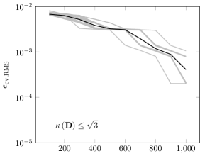
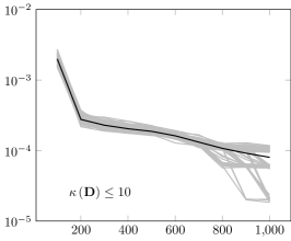
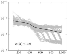
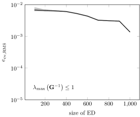
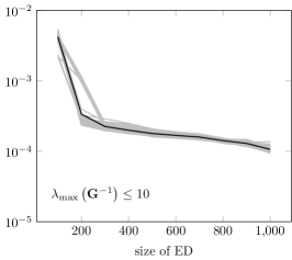
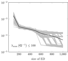
Figure 3: RMS CV errors of PCEs approximating the single-frequency dielectric-inset rectangular waveguide model, for EDs of increasing size and different sequential ED criteria. The gray lines show the results of 100 different EDs. The average errors are shown in black.

In most UQ studies for frequency-response models, such as the waveguide examined here, one PCE per frequency point is developed in order to approximate the model’s response over a frequency range. Therefore, in this first numerical experiment, we will approximate the functional $r(\mathbf{y})$, given in decibels, for a fixed frequency $f=5$ GHz. In particular, we employ Algorithm 2 using 3 different condition number limits, 3 different maximum eigenvalue limits and 3 different maximum trace limits, with respect to the sequential expansion of the ED. We construct PCEs using $100$ different random EDs, i.e., using different random sampling seeds. The RMS CV error (16) is computed using a random sample with $Q=10^{5}$ points. The approximation results are shown in Figure 3, where we omit the trace-related results, since they follow closely the eigenvalue-related ones. Each subplot corresponds to a different sequential ED criterion and shows the RMS CV error of the PCEs for EDs of increasing size. In all cases, the surrogate models reach accuracies well beyond the ones typically needed in engineering applications.

Looking at the first two columns of Figure 3, it can be indeed observed that more relaxed criteria improve the accuracy of the PCE on average. Relaxing the condition-number criterion from $\kappa\left(\mathbf{D}\right)\leq\sqrt{3}$ to $\kappa\left(\mathbf{D}\right)\leq 10$ does not seem to introduce larger variations with respect to the PCEs’ accuracy. A more pronounced difference is observed between the eigenvalue-based criteria $\lambda_{\max}\leq 1$ and $\lambda_{\max}\leq 10$, however, the PCEs can in both cases be regarded as robust. The rightmost columns of Figure 3 show that further relaxation of the criteria results in either marginal gains (bottom row), or in accuracy deterioration (top row). Comparing the top and bottom-row sub-figures, the eigenvalue-based criteria seem to result in more robust results for a similar accuracy-cost relation. In terms of a compromise between costs and accuracy, the best choices regarding the sequential expansion of the ED are found to be $\kappa\left(\mathbf{D}\right)\leq 10$ and $\lambda_{\max}\leq 10$, for this particular model. However, we should note that PCEs based on the strictest and most robust criteria, i.e., $\kappa\left(\mathbf{D}\right)\leq\sqrt{3}$ and $\lambda_{\max}\leq 1$, also yield errors below the engineering standards, on top of being more robust in their results.

4.2.2 Broadband Surrogate Modeling

As mentioned in Section 4.2.1, the frequency response is typically approximated using one PCE per frequency point, equivalently, per time step in time-domain approaches [62, 52]. This can be computationally expensive in cases where a large number of frequency points must be examined. For high-frequency models where the frequency dependence is also a relatively smooth functional, e.g., no sharp resonances exist in the examined frequency range, one can extend the presented surrogate modeling approach, such that it includes the frequency dependence as well [21]. Specifically, while not random, the frequency can be modeled as a parameter which is uniformly distributed in the specified frequency range. The resulting PCE approximates the functional $r(f,\mathbf{y})$, including the frequency dependence next to the geometrical and material parameters.

Using this idea, we repeat the numerical experiments of Section 4.2.1, where the frequency is now an additional uniformly distributed parameter in the range $\left[10,20\right]$ GHz. The results are shown in Figure 4. The surrogate models reach satisfactory accuracies for the whole frequency range. Similar to the single-frequency case, the eigenvalue-based criteria seem to be more robust compared to the condition-number-based ones, for a similar accuracy-cost relation. Once more, the conditions $\kappa\left(\mathbf{D}\right)\leq 10$ and $\lambda_{\max}\left(\mathbf{G}^{-1}\right)\leq 10$ yield the best compromises between approximation accuracy and robustness. In both cases, further relaxation of the sequential ED criteria not only adds significant variation in the results, but also worsens the average accuracy.

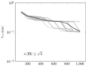
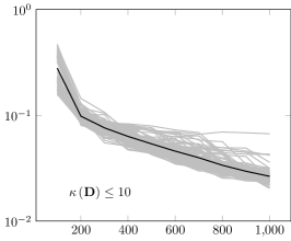
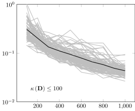
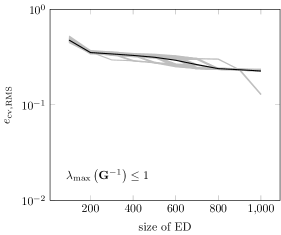
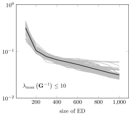
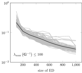
Figure 4: RMS CV errors of PCEs approximating the broadband dielectric-inset rectangular waveguide model, for EDs of increasing size and different sequential ED criteria. The gray lines show the results of 100 different EDs. The average errors are shown in black.

4.3 Optical Grating Coupler

For the next, more challenging numerical example, we use a $1$D grating coupler model [51]. Such nanometer-scaled devices are employed in the field of nano-photonics and plasmonics [53, 1, 2]. Their multi-layer structure consists of a high index dielectric on top of a metallic grating, which is placed on a substrate. A simplified, schematic model is depicted in Figure 6. We assume the structure to be infinitely extended in the lateral directions. Furthermore, only normal incident light beams from the top are considered. For certain incident wavelengths, matching the geometry dimensions, surface plasmons are excited in the metallic grating. Those wavelengths can be detected by observing the reflection coefficient $r$, which shows a dip in the frequency response each time the condition is satisfied, i.e., when a surface plasmon is excited, see Figure 6. Note that, due to the resonances, a polynomial approximation of the grating coupler model including the frequency-responce becomes significantly more challenging.

The surface plasmon coupling is highly sensitive to the coupler’s geometrical parameters, in particular, the grating pitch length $d_{\mathrm{G}}$, the groove $a_{\mathrm{G}}$, the thickness of the metallic and dielectric layers $h_{\mathrm{m}}$, respectively, $h_{\mathrm{D}}$, as well as the grating thickness $h_{\mathrm{G}}$ (see Figure 6). A full parameter study can be found in [51]. Following the same work, we model those four parameters as uniformly distributed and independent RVs, such that $Y_{n}\sim\mathcal{U}[\bar{y}_{n}-\delta_{y_{n}},\bar{y}_{n}+\delta_{y_{n}}]$, where $\bar{y}_{n}$ denotes the nominal value and $\delta_{y_{n}}$ the maximum allowed deviation from the nominal value. The parameters, their nominal values, and the allowed deviations are shown in Table 2.

4.3.1 Broadband Surrogate Modeling

In this example, we only consider the broadband approximation of the grating coupler model, similar to Section 4.2.2. Thus, we model the wavelength as uniformly distributed in $\left[$550\text{\,}\mathrm{nm}$,$800\text{\,}\mathrm{nm}$\right]$. For a given realization of the parameter vector $\mathbf{y}=\mathbf{Y}\left(\theta\right)$ and a wavelength value $\lambda$, the reflection coefficient is a deterministic QoI denoted by $r(\lambda,\mathbf{y})$ and given in decibels. For the computation of the reflection coefficient, we employ a rigorous coupled wave analysis (RCWA) code [26, 37].

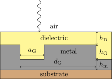
Figure 5: Schematic view of the optical grating coupler.

Figure 6: Frequency-response of the optical grating coupler for the nominal geometry parameters.

Table 2: Uncertain geometric parameters of the grating structure.

parameter mean $\bar{y}\left[$\text{\,}\mathrm{nm}$\right]$ variation $\delta_{y}\left[$\text{\,}\mathrm{nm}$\right]$ $h_{\mathrm{D}}$ $84.8$ $0.3$ $h_{\mathrm{G}}$ $68.1$ $0.1$ $d_{\mathrm{G}}$ $499.2$ $1.0$ $a_{\mathrm{G}}$ $165.4$ $1.5$

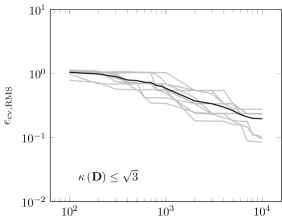
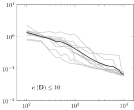
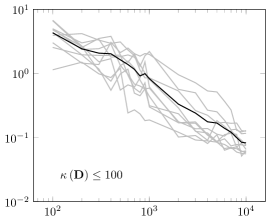
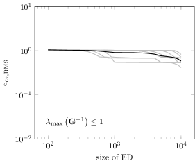
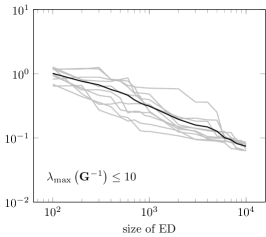
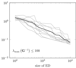
Figure 7: RMS CV errors of PCEs approximating the broadband grating coupler model, for EDs of increasing size and different sequential ED criteria. The gray lines show the results of 10 different EDs. The average errors are shown in black.

Numerical results for different sequential ED conditions are depicted in Figure 7. Once more, we omit the trace-based criterion, as the corresponding results are similar to the eigenvalue-based ones. Despite the non-smooth frequency response, our method is able to provide accurate approximations, albeit at an elevated cost, i.e., EDs with up to $10^{4}$ parameter realizations are employed. It is worth stating that the resonances do not render PCEs altogether inapplicable, as is often the case for non-smooth responses. Additionally considering the higher computational cost of the RCWA solver, we employ only $10$ different EDs. The size of the CV sample used for computing the error (16) remains equal to $Q=10^{5}$.

Similar to the results of Section 4.2, relaxed sequential ED criteria improve the average approximation accuracy, and at the same time introduce a larger variation among PCEs constructed for different EDs, as can be observed from the first two columns of Figure 6. The last column of Figure 6 shows once more that, after a certain point, further relaxation of the sequential ED criteria only enlarges the variation without accuracy improvement. Once again, the eigenvalue-based criteria yield more robust results compared to the condition-number-based ones, however, the difference is not as pronounced as in Section 4.2. Moreover, using the criterion $\lambda_{\max}(\mathbf{G}^{-1})\leq 1$, almost no accuracy improvement is obtained for larger datasets. Similar to Section 4.2, the conditions $\kappa(\mathbf{D})\leq 10$ and $\lambda_{\max}(\mathbf{G}^{-1})\leq 10$ provide the best trade-off between accuracy and robustness.

5 Summary and Conclusions

In this work, we proposed an algorithm to construct sparse LS-based PCEs. The algorithm features a sensitivity-based, adaptive selection of the polynomial basis terms, as well as a sequential ED strategy, such that the available dataset of parameter realizations and QoI observations is expanded at wish, given different optimality criteria. We focused on three such criteria, namely $K$-, $E$- and $A$-optimality, to construct nested datasets of EDs and observations, and investigated the influence of different optimality conditions on the accuracy and robustness of the PCE-based surrogate models.

The method’s accuracy and efficiency has been verified on two high-frequency electromagnetic models. Although comparisons between our approach and competitive methods, either non-adaptive or adaptive, have not been presented here, our method typically outperforms fixed-degree PCE approaches by orders and has been found to be superior to the popular least angle regression (LAR)-PCE approach [40]. Instead, this work focused on the largely unexplored topic of PCE robustness, which is closely related to the stability of the discrete LS regression problem. In turn, LS stability can be quantified by certain algebraic measures of the corresponding information matrix, with each of these measures being related to a so-called optimal ED criterion. It was repeatedly shown that strict criteria result in robust PCEs, the accuracy of which remains relatively unaffected by the given dataset. Relaxing those criteria can improve the on-average accuracy at the cost of robustness, i.e., resulting in larger variations among PCEs constructed with different datasets. Relaxation of the sequential ED criteria beyond a certain point only introduces more variation, while at the same time not improving or even worsening the average PCE accuracy. In all numerical experiments, a good accuracy-robustness trade-off has been acquired with the criteria $\kappa\left(\mathbf{D}\right)\leq 10$ and $\lambda_{\max}\left(\mathbf{G}^{-1}\right)\leq 10$, the latter being typically more robust for approximations of similar accuracy. Compared to the theoretically optimal condition $\kappa\left(\mathbf{G}\right)\leq 3$ [12, 13, 46, 44], equivalently, $\kappa\left(\mathbf{D}\right)\leq\sqrt{3}$, our results show that those relaxed criteria yield significant accuracy gains, while keeping result variations at a modest level.

A continuation of the present work shall focus on developing surrogate models for high frequency EM applications featuring sharp resonances. In such cases, most polynomial approximations will fail to accurately capture the frequency response. A possible remedy could be found in multi-element PCE methods [33, 59, 58], which are able to yield accurate approximations of non-smooth, discontinuous, or even singular parametric functions. This approach is currently under investigation and will be presented in a later study.

Acknowledgment

D. Loukrezis and H. De Gersem would like to acknowledge the support of the Graduate School of Excellence for Computational Enginering at the Technische Universität Darmstadt. D. Loukrezis further acknowledges the support of the BMBF via the research contract 05K19RDB. A. Galetzka’s work is supported by the DFG through the Graduiertenkolleg 2128 “Accelerator Science and Technology for Energy Recovery Linacs ”.

References

- [1] G. M. Akselrod, C. Argyropoulos, T. B. Hoang, C. Ciracì, C. Fang, J. Huang, D. R. Smith, and M. H. Mikkelsen. Probing the mechanisms of large purcell enhancement in plasmonic nanoantennas. Nature Photonics, 8:835 EP –, Oct 2014.
- [2] G. M. Akselrod, T. Ming, C. Argyropoulos, T. B. Hoang, Y. Lin, X. Ling, D. R. Smith, J. Kong, and M. H. Mikkelsen. Leveraging nanocavity harmonics for control of optical processes in 2d semiconductors. Nano Letters, 15(5):3578–3584, 2015. PMID: 25914964.
- [3] B. Arras, M. Bachmayr, and A. Cohen. Sequential sampling for optimal weighted least squares approximations in hierarchical spaces. SIAM Journal on Mathematics of Data Science, 1(1):189–207, 2019.
- [4] I. Babuška, F. Nobile, and R. Tempone. A stochastic collocation method for elliptic partial differential equations with random input data. SIAM Review, 52(2):317–355, 2010.
- [5] M. Baudin, A. Dutfoy, B. Iooss, and A.-L. Popelin. OpenTURNS: An industrial software for uncertainty quantification in simulation. In R. Ghanem, D. Higdon, and H. Owhadi, editors, Handbook of Uncertainty Quantification, pages 2001–2038. Springer International Publishing, 2017.
- [6] R. E. Bellman. Dynamic Programming. Princeton University Press, 1957.
- [7] G. Blatman and B. Sudret. An adaptive algorithm to build up sparse polynomial chaos expansions for stochastic finite element analysis. Probabilistic Engineering Mechanics, 25(2):183–197, 2010.
- [8] G. Blatman and B. Sudret. Efficient computation of global sensitivity indices using sparse polynomial chaos expansions. Reliability Engineering and System Safety, 95(11):1216 – 1229, 2010.
- [9] G. Blatman and B. Sudret. Adaptive Sparse Polynomial Chaos Expansion Based on Least Angle Regression. Journal of Computational Physics, 230(6):2345–2367, 2011.
- [10] E. Burnaev, I. Panin, and B. Sudret. Efficient design of experiments for sensitivity analysis based on polynomial chaos expansions. Annals of Mathematics and Artificial Intelligence, 81(1):187–207, Oct 2017.
- [11] R. E. Caflisch. Monte Carlo and quasi-Monte Carlo methods. Acta Numerica, 7:1 – 49, 1998.
- [12] A. Chkifa, A. Cohen, G. Migliorati, F. Nobile, and R. Tempone. Discrete least squares polynomial approximation with random evaluations - application to parametric and stochastic elliptic pdes. ESAIM: M2AN, 49(3):815–837, 2015.
- [13] A. Cohen, M. A. Davenport, and D. Leviatan. On the stability and accuracy of least squares approximations. Foundations of Computational Mathematics, 13(5):819–834, 2013.
- [14] A. Cohen and G. Migliorati. Optimal weighted least-squares methods. SMAI Journal of Computational Mathematics, 3:181–203, 2017.
- [15] A. Cohen and G. Migliorati. Multivariate approximation in downward closed polynomial spaces. In J. Dick, F. Y. Kuo, and H. Woźniakowski, editors, Contemporary Computational Mathematics - A Celebration of the 80th Birthday of Ian Sloan, Springer International Publishing, pages 233–282, 2018.
- [16] P. Diaz, A. Doostan, and J. Hampton. Sparse polynomial chaos expansions via compressed sensing and d-optimal design. Computer Methods in Applied Mechanics and Engineering, 336:640 – 666, 2018.
- [17] A. Doostan and H. Owhadi. A non-adapted sparse approximation of pdes with stochastic inputs. Journal of Computational Physics, 230(8):3015 – 3034, 2011.
- [18] A. Doostan, A. Validi, and G. Iaccarino. Non-intrusive low-rank separated approximation of high-dimensional stochastic models. Computer Methods in Applied Mechanics and Engineering, 263:42 – 55, 2013.
- [19] N. Fajraoui, S. Marelli, and B. Sudret. Sequential design of experiment for sparse polynomial chaos expansions. SIAM/ASA Journal on Uncertainty Quantification, 5(1):1061–1085, 2017.
- [20] J. Feinberg, V. Eck, and H. Langtangen. Multivariate polynomial chaos expansions with dependent variables. SIAM Journal on Scientific Computing, 40(1):A199–A223, 2018.
- [21] N. Georg, D. Loukrezis, U. Römer, and S. Schöps. Uncertainty quantification for an optical grating coupler with an adjoint-based leja adaptive collocation method. CoRR, abs/1807.07485, 2018.
- [22] T. Gerstner and M. Griebel. Dimension-Adaptive Tensor-Product Quadrature. Computing, 71(1):65–87, 2003.
- [23] R. G. Ghanem and P. D. Spanos. Stochastic Finite Elements: A Spectral Approach. Springer-Verlag New York, Inc, New York, NY, USA, 1991.
- [24] K. T. Gladwin Jos and K. J. Vinoy. A fast polynomial chaos expansion for uncertainty quantification in stochastic electromagnetic problems. IEEE Antennas and Wireless Propagation Letters, pages 1–1, 2019.
- [25] G. H. Golub and C. F. Van Loan. Matrix Computations (3rd Ed.). Johns Hopkins University Press, Baltimore, MD, USA, 1996.
- [26] G. Granet and B. Guizal. Efficient implementation of the coupled-wave method for metallic lamellar gratings in tm polarization. Journal of the Optical Society of America A, 13(5):1019–1023, May 1996.
- [27] M. Hadigol and A. Doostan. Least squares polynomial chaos expansion: A review of sampling strategies. Computer Methods in Applied Mechanics and Engineering, 332:382 – 407, 2018.
- [28] J. Hampton and A. Doostan. Coherence motivated sampling and convergence analysis of least squares polynomial chaos regression. Computer Methods in Applied Mechanics and Engineering, 290:73 – 97, 2015.
- [29] J. Hampton and A. Doostan. Compressive sampling of polynomial chaos expansions: Convergence analysis and sampling strategies. Journal of Computational Physics, 280:363 – 386, 2015.
- [30] N. J. Higham. Accuracy and Stability of Numerical Algorithms. Society for Industrial and Applied Mathematics, second edition, 2002.
- [31] R. Hu, V. Monebhurrun, R. Himeno, H. Yokota, and F. Costen. An adaptive least angle regression method for uncertainty quantification in fdtd computation. IEEE Transactions on Antennas and Propagation, 66(12):7188–7197, Dec 2018.
- [32] J. D. Jakeman, M. S. Eldred, and K. Sargsyan. Enhancing -minimization estimates of polynomial chaos expansions using basis selection. Journal of Computational Physics, 289:18 – 34, 2015.
- [33] J. D. Jakeman, A. Narayan, and D. Xiu. Minimal multi-element stochastic collocation for uncertainty quantification of discontinuous functions. Journal of Computational Physics, 242:790 – 808, 2013.
- [34] R. Jankoski, U. Römer, and S. Schöps. Stochastic modeling of magnetic hysteretic properties by using multivariate random fields. International Journal for Uncertainty Quantification, 9(1):85–102, 2019.
- [35] K. Konakli and B. Sudret. Global sensitivity analysis using low-rank tensor approximations. Reliability Engineering & System Safety, 156:64 – 83, 2016.
- [36] K. Konakli and B. Sudret. Polynomial meta-models with canonical low-rank approximations: Numerical insights and comparison to sparse polynomial chaos expansions. Journal of Computational Physics, 321:1144 – 1169, 2016.
- [37] P. Lalanne and G. M. Morris. Highly improved convergence of the coupled-wave method for tm polarization. Journal of the Optical Society of America A, 13(4):779–784, Apr 1996.
- [38] R. Lebrun and A. Dutfoy. A generalization of the nataf transformation to distributions with elliptical copula. Probabilistic Engineering Mechanics, 24(2):172 – 178, 2009.
- [39] C. Lemieux. Monte Carlo and Quasi-Monte Carlo Sampling. Springer Series in Statistics. 2009.
- [40] D. Loukrezis. Adaptive approximations for high-dimensional uncertainty quantification in stochastic parametric electromagnetic field simulations. PhD thesis, Technische Universität Darmstadt, 2019.
- [41] D. Loukrezis, U. Römer, and H. De Gersem. Assessing the performance of Leja and Clenshaw-Curtis collocation for computational electromagnetics with random input data. International Journal for Uncertainty Quantification, 9(1):33–57, 2019.
- [42] G. Migliorati. Adaptive Polynomial Approximation by Means of Random Discrete Least Squares. In A. Abdulle, S. Deparis, D. Kressner, F. Nobile, and M. Picasso, editors, ENUMATH, volume 103 of Lecture Notes in Computational Science and Engineering, pages 547–554. Springer, 2013.
- [43] G. Migliorati. Learning with discrete least squares on multivariate polynomial spaces using evaluations at random or low-discrepancy point sets. In P. Pardalos, M. Pavone, G. M. Farinella, and V. Cutello, editors, Machine Learning, Optimization, and Big Data, pages 1–13. Springer International Publishing, 2015.
- [44] G. Migliorati and F. Nobile. Analysis of discrete least squares on multivariate polynomial spaces with evaluations at low-discrepancy point sets. Journal of Complexity, 31(4):517–542, 2015.
- [45] G. Migliorati, F. Nobile, E. von Schwerin, and R. Tempone. Approximation of Quantities of Interest in Stochastic PDEs by the Random Discrete L2 Projection on Polynomial Spaces. SIAM Journal on Scientific Computing, 35(3), 2013.
- [46] G. Migliorati, F. Nobile, E. von Schwerin, and R. Tempone. Analysis of Discrete L2 Projection on Polynomial Spaces with Random Evaluations. Foundations of Computational Mathematics, 14(3):419–456, 2014.
- [47] T. T. Nguyen, D. H. Mac, and S. Clénet. Uncertainty quantification using sparse approximation for models with a high number of parameters: Application to a magnetoelectric sensor. IEEE Transactions on Magnetics, 52(3):1–4, March 2016.
- [48] P. Offermann, H. Mac, T. T. Nguyen, S. Clénet, H. De Gersem, and K. Hameyer. Uncertainty quantification and sensitivity analysis in electrical machines with stochastically varying machine parameters. IEEE Transactions on Magnetics, 51(3):1–4, March 2015.
- [49] S. Oladyshkin and W. Nowak. Data-driven uncertainty quantification using the arbitrary polynomial chaos expansion. Reliability Engineering & System Safety, 106:179–190, 2012.
- [50] J. Peng, J. Hampton, and A. Doostan. A weighted l1-minimization approach for sparse polynomial chaos expansions. Journal of Computational Physics, 267:92 – 111, 2014.
- [51] A. Pitelet, N. Schmitt, D. Loukrezis, C. Scheid, H. D. Gersem, C. Ciracì, E. Centeno, and A. Moreau. Influence of spatial dispersion on surface plasmons, nanoparticles, and grating couplers. Journal of the Optical Society of America B, 36(11):2989–2999, Nov 2019.
- [52] A. K. Prasad, M. Ahadi, and S. Roy. Multidimensional uncertainty quantification of microwave/rf networks using linear regression and optimal design of experiments. IEEE Transactions on Microwave Theory and Techniques, 64(8):2433–2446, Aug 2016.
- [53] J. A. Schuller, E. S. Barnard, W. Cai, Y. C. Jun, J. S. White, and M. L. Brongersma. Plasmonics for extreme light concentration and manipulation. Nature Materials, 9(3):193–204, 2010.
- [54] R. Smith. Uncertainty Quantification: Theory, Implementation, and Applications. Computational Science and Engineering, SIAM. 2014.
- [55] C. Soize and R. Ghanem. Physical systems with random uncertainties: Chaos representations with arbitrary probability measure. SIAM Journal on Scientific Computing, 26(2):395–410, 2004.
- [56] B. Sudret. Global sensitivity analysis using polynomial chaos expansions. Reliability Engineering & System Safety, 93(7):964 – 979, 2008.
- [57] T. J. Sullivan. Introduction to Uncertainty Quantification. Texts in Applied Mathematics, Springer International Publishing Switzerland. 2015.
- [58] X. Wan and G. Karniadakis. Multi-Element Generalized Polynomial Chaos for Arbitrary Probability Measures. SIAM Journal on Scientific Computing, 28(3):901–928, 2006.
- [59] X. Wan and G. E. Karniadakis. An adaptive multi-element generalized polynomial chaos method for stochastic differential equations. Journal of Computational Physics, 209(2):617 – 642, 2005.
- [60] X. Wan and G. E. Karniadakis. Beyond Wiener–Askey expansions: Handling arbitrary PDFs. Journal of Scientific Computing, 27(1):455–464, Jun 2006.
- [61] D. Xiu and G. E. Karniadakis. The Wiener-Askey Polynomial Chaos for Stochastic Differential Equations. SIAM Journal on Scientific Computing, 24(2):619–644, 2002.
- [62] J. Xu, M. Y. Koledintseva, Y. Zhang, Y. He, B. Matlin, R. E. DuBroff, J. L. Drewniak, and J. Zhang. Complex permittivity and permeability measurements and finite-difference time-domain simulation of ferrite materials. IEEE Transactions on Electromagnetic Compatibility, 52(4):878–887, Nov 2010.