PETSc TSAdjoint: a discrete adjoint ODE solver for first-order and second-order sensitivity analysis This material is based upon work supported by the U.S. Department of Energy, Office of Science, Office of Advanced Scientific Computing Research, Scientific Discovery through Advanced Computing (SciDAC) program through the FASTMath Institute under contract DE-AC02-06CH11357 at Argonne National Laboratory.

Abstract

We present a new software system PETSc TSAdjoint for first-order and second-order adjoint sensitivity analysis of time-dependent nonlinear differential equations. The derivative calculation in PETSc TSAdjoint is essentially a high-level algorithmic differentiation process. The adjoint models are derived by differentiating the timestepping algorithms and implementing them based on the parallel infrastructure in PETSc. Full differentiation of the library code, including MPI routines, is avoided, and users do not need to derive their own adjoint models for their specific applications. PETSc TSAdjoint can compute the first-order derivative, that is, the gradient of a scalar functional, and the Hessian-vector product, which carries second-order derivative information, while requiring minimal input (a few callbacks) from the users. The adjoint model employs optimal checkpointing schemes in a manner that is transparent to users. Usability, efficiency, and scalability are demonstrated through examples from a variety of applications.

97N80, 65L99, 49Q12

1 Introduction

Adjoint methods have been used extensively in computational modeling and optimization, playing a key role in neural networks, sensitivity analysis, goal-oriented error estimation, data assimilation, and optimal control. They are efficient algorithmic differentiation (AD) approaches for computing the derivatives of an objective function of the solution of an ordinary differential equation (ODE) or differential-algebraic equation (DAE) with respect to parameters of interest, with a cost independent of the number of parameters. Deriving the adjoint model is trivial for linear models but can be difficult for nonlinear models [15], especially time-dependent problems.

Many tools have been developed to derive and implement adjoint models automatically. These automatic tools take as input a forward model that users implement in languages such as C [8, 37], C++ [6], Fortran [18], Python [27], and Julia [24]; and they produce as output the associated discrete adjoint model in a line-by-line fashion, through source-to-source transformations, operator overloading, or a combination of both. While this black-box approach gives the highest degree of automation and requires the least knowledge of the mathematical models, it suffers from many low-level implementation-specific difficulties including memory allocation, management of pointers, input/output, and parallel communication (e.g., MPI and OpenMP). Such black-box tools also often produce far from optimally efficient code.

Traditional AD treats a model as a sequence of primitive instructions (e.g., addition, multiplication, logarithm) and calculates the derivatives based on the chain rule using the derivatives of these primitive instructions, which are easily obtainable. In order to overcome the difficulties of these low-level approaches, high-level AD libraries such as dolfin-adjoint [15] and FATODE [41] recently have been developed to operate at high abstraction levels.

The landscape of popular existing AD software is depicted in Figure 1. While these software packages are developed based on the same theory, they differ significantly in usage and require varying levels of effort from developers and users. Dolfin-adjoint [15] considers a model as a sequence of nonlinear equation solves in the form $A(u)u=b(u)$, where $u$ is the vector of all prognostic variables, $b(u)$ is the source term, and $A(u)$ is the entire discretization matrix. The derivation of the adjoint model is fully automated in dolfin-adjoint if the forward model is written in a high-level language that is similar to mathematical notation. Dolfin-adjoint is used primarily by finite-element systems such as FEniCS [3] and Firedrake [31]. FATODE implements an adjoint model by considering the algorithm of solving time-dependent differential equations as a sequence of timestepping solves. FATODE provides a built-in implementation of the adjoint model derived based on the timestepping algorithms for solving ODEs; simulation of time-dependent partial differential equations (PDEs) is abstracted as a sequence of time steps, and the libraries differentiate each time step. In contrast, the adjoint solvers CVODES and IDAS in the SUNDIALS [21] package, which have been used by notable optimization tools such as CasADi [4], implement an adjoint model that users derive directly from the model equations. This highest-level approach, also known as the continuous adjoint approach, requires users to derive a new set of equations before discretization (adjoint model of the original continuum or weak form mode). All the other aforementioned approaches are discrete adjoint approaches since the adjoint models are derived after discretization. In general, lower-level abstractions tend to impose more implementation burden on library developers and provide more automation to users while, at the same time, hiding more mathematical structures from users. Nevertheless, low-level AD can be mixed with high-level AD to improve scaling. For example, the internal Jacobian-vector product in a high-level AD implementation can be effectively computed by using the traditional reverse-mode AD. This approach has been adopted in many works [4, 28, 36].

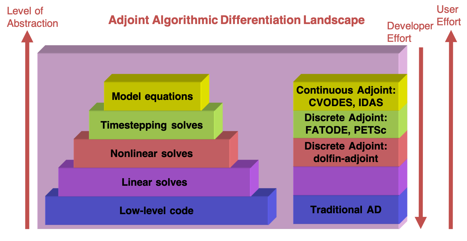
Figure 1: Landscape of adjoint algorithmic differetiation software.

Another tool that has recently been developed is a Julia library called DifferentialEquations.jl [29]. It has support for both continuous and discrete first-order adjoint sensitivity analysis for ODEs, and experimental support for second-order sensitivity analysis is claimed.

Adopting a similar approach to that used by FATODE, we have developed the TSAdjoint component in the Portable, Extensible Toolkit for Scientific Computation PETSc [1, 39]. PETSc TSAdjoint enables first- and second-order adjoint sensitivity analysis for nonlinear time-dependent differential equations, which are the key ingredients of many optimization algorithms. The adjoint models are derived and implemented for various time integrators in PETSc in a manner that is agnostic to the spatial discretization engine, thus being suitable for general-purpose applications. The adjoint models also employ the parallel infrastructure and the sophisticated linear/nonlinear solvers in PETSc in the same way as the forward models. Optimal adjoint checkpointing schemes are implemented and tailored to the needs of the ODE/DAE solvers. The adjoint control flow is managed automatically by PETSc and is transparent to users. These features are significant advantages in achieving the efficiency of adjoint calculation compared with other adjoint codes. In particular, dolfin-adjoint covers less general applications. FATODE, CVODES, IDAS and DifferentialEquations.jl lack support for optimal checkpointing; and to the best of our knowledge, there are no reported demonstrations or attempts to use state-of-the-art linear/nonlinear solvers with these tools, although they are generic to the internal linear solver. A drawback with TSAdjoint is that the adjoint of each timestepping algorithm must be implemented by the library developers.

In the next section, we provide the mathematical foundations of sensitivity analysis for ODE integrators. In Section 3, we explain the software infrastructure. Section 4 discusses the management of the required checkpointing, and Section 5 explores the use of these algorithms in three examples. Section 6 summarizes our conclusions.

2 Mathematical Foundation

This section explains how the sensitivity propagation equations are derived based on the model abstraction at the timestepping level. Both first-order and second-order sensitivity analysis approaches are covered. An example using theta timestepping methods, for which the adjoint model has moderate complexity, is given to illustrate the details of the derivation. The mathematical framework can be naturally extended to other timestepping algorithms, including explicit schemes and even implicit-explicit schemes.

The goal of sensitivity analysis of a dynamical system is to compute the derivative of a scalar functional with respect to specific system parameters. We consider the dynamical system in DAE form for notational brevity and without loss of generality:

(1) $$\bm{\mathcal{M}}\dot{\bm{u}}=\bm{f}(t,\bm{u};\bm{p})\,,$$

where $\bm{\mathcal{M}}\in\mathbb{R}^{N_{d}\times N_{d}}$ is the mass matrix, $\bm{u}\in\mathbb{R}^{N_{d}}$ is the system state, and $\bm{p}\in\mathbb{R}^{N_{p}}$ are the parameters of interest. These forms typically arise from the semi-discretization of time-dependent PDEs using the method of lines. The mass matrix may be the identity for typical ODEs or a singular matrix for DAEs. In this paper, vectors and matrices are denoted by bold letters and scalars by non-bold letters. The numerator layout notation is used for derivatives; for example, the derivative of a scalar function is a row vector.

Consider time integration as a sequence of operations,

(2) $$\bm{u}_{n+1}=\bm{\mathcal{N}}(\bm{u}_{n}),\quad n=0,\dots,N-1,$$

where the initial condition is $\bm{u}_{0}=\bm{\mathcal{\eta}}$ and $\bm{\mathcal{N}}$ is a timestepping operator that propagates the solution from $t_{n}$ to $t_{n+1}$. An example of $\bm{\mathcal{N}}$, an implicit timestepping method, is discussed in Section 2.4. The scalar functional in sensitivity analysis depends on the system states and is denoted by $\psi(\bm{u}_{N})$ if it is a function of the final state or expressed in integral form

(3) $$\int_{t_{0}}^{t_{F}}r(t,\bm{u};\bm{p})dt$$

if it is a function of the entire trajectory of the system.

In the following two subsections, we briefly explain how the derivatives of a scalar function $\psi(\bm{u}_{N})$ with respect to the initial condition are derived in the discrete regime. The derivatives with respect to parameters (e.g., model parameters) can be derived with the same framework by augmenting the parameters into the initial condition vector. We refer readers to [41] for details.

2.1 First-order discrete derivatives

We use the Lagrange multipliers $\bm{\lambda}_{n}\in\mathbb{R}^{N_{d}},n=0,\dots,N$, which are column vectors, to account for the constraint from each time step and define the Lagrangian

(4) $$\mathcal{L}(\bm{\mathcal{\eta}})=\psi(\bm{u}_{N})-\bm{\lambda}_{0}^{T}\left(\bm{u}_{0}-\bm{\mathcal{\eta}}\right)-\sum_{n=0}^{N-1}\bm{\lambda}_{n+1}^{T}\left(\bm{u}_{n+1}-\bm{\mathcal{N}}(\bm{u}_{n})\right).$$

We choose the transpose for the convenience of derivation because the derivative of a row vector with respect to a column vector is not well defined in matrix calculus.

Taking the total derivative of equation (4) with respect to the initial condition $\bm{\mathcal{\eta}}$ leads to

(5) $$\dfrac{d\mathcal{L}}{d\bm{\mathcal{\eta}}}=\bm{\lambda}_{0}^{T}-\left(\frac{d\psi}{d\bm{u}}(\bm{u}_{N})-\bm{\lambda}_{N}^{T}\right)\frac{d\bm{u}_{N}}{d\bm{\mathcal{\eta}}}-\sum_{n=0}^{N-1}\left(\bm{\lambda}_{n}^{T}-\bm{\lambda}_{n+1}^{T}\frac{d\bm{\mathcal{N}}}{d\bm{u}}(\bm{u}_{n})\right)\frac{d\bm{u}_{n}}{d\bm{\mathcal{\eta}}}.$$

The first-order adjoint equation is defined as

(6) $$\bm{\lambda}_{n} =\left(\frac{d\bm{\mathcal{N}}}{d\bm{u}}(\bm{u}_{n})\right)^{T}\bm{\lambda}_{n+1},\quad n=N-1,\dots,0,$$

$$\bm{\lambda}_{N} =\left(\frac{d\psi}{d\bm{u}}(\bm{u}_{N})\right)^{T},$$

in order to make the last two terms in (5) vanish so that the total derivative can be obtained without computing the forward sensitivities. Note that in the adjoint model, the sensitivities are calculated by propagating the derivative information in reverse order.

An alternative approach is to derive the discrete tangent linear model (TLM) from the discrete forward model. By differentiating directly (2) with respect to the initial condition $\bm{\mathcal{\eta}}$ and defining the sensitivity matrix $\bm{\mathcal{S}}_{n}\in\mathbb{R}^{N_{d}\times N_{d}}$ by

(7) $$\bm{\mathcal{S}}_{n}=\frac{d\bm{u}_{n}}{d\bm{\mathcal{\eta}}},\quad n=0,\dots,N-1,$$

we can obtain the TLM equations

(8) $$\bm{\mathcal{S}}_{n+1}=\left(\frac{d\bm{\mathcal{N}}}{d\bm{u}}(\bm{u}_{n})\right)\,\bm{\mathcal{S}}_{n},\quad n=0,\dots,N-1,$$

which propagates the sensitivity matrix forward in time and can be solved together with the original model equations (1). Similarly, one can differentiate (2) with respect to the parameters to derive the TLM equations for calculating parameter sensitivities. These sensitivities can be used to compute the derivative of the scalar functional through the chain rule so that the TLM method can achieve the same goal as the adjoint method. However, these two methods may differ significantly in terms of computational cost. The computational complexity of the adjoint method is $\mathcal{O}(N_{f})$ whereas the complexity of the TLM method is $\mathcal{O}(N_{p})$, where $N_{f}$ and $N_{p}$ are the number of functionals and the number of parameters, respectively. Therefore, the adjoint method is more efficient than the TLM method when computing derivatives of a scalar functional with respect to many parameters. The TLM method can be efficient only when there are few parameters and has limited application compared with the adjoint method.

2.2 Second-order discrete derivatives

A most computationally efficient approach for calculating second-order derivatives for a large number of parameters is the forward-over-adjoint method [2], which requires both the first-order adjoint model and the TLM. By differentiating the transpose of $\dfrac{d\mathcal{L}}{d\bm{\mathcal{\eta}}}$ with respect to $\bm{\mathcal{\eta}}$ for a second time, we obtain

(9) $$\dfrac{d}{d\bm{\mathcal{\eta}}}\left(\dfrac{d\mathcal{L}}{d\bm{\mathcal{\eta}}}\right)^{T} =\frac{d\bm{\lambda}_{0}}{d\bm{\mathcal{\eta}}}-\left(\frac{d\psi}{d\bm{u}}(\bm{u}_{N})-\bm{\lambda}_{N}^{T}\right)\frac{d^{2}\bm{u}_{N}}{d\bm{\mathcal{\eta}}^{2}}$$

$$-\left(\frac{d\bm{u}_{N}}{d\bm{\mathcal{\eta}}}\right)^{T}\left(\frac{d}{d\bm{u}}\left(\frac{d\psi}{d\bm{u}}(\bm{u}_{N})\right)^{T}\frac{d\bm{u}_{N}}{d\bm{\mathcal{\eta}}}-\frac{d\bm{\lambda}_{N}}{d\bm{\mathcal{\eta}}}\right)$$

$$-\sum_{n=0}^{N-1}\left(\frac{d\bm{u}_{n}}{d\bm{\mathcal{\eta}}}\right)^{T}\left(\frac{d\bm{\lambda}_{n}}{d\bm{\mathcal{\eta}}}-\bm{\lambda}_{n+1}^{T}\,\frac{d^{2}\bm{\mathcal{N}}}{d\bm{u}^{2}}(\bm{u}_{n})\,\frac{d\bm{u}_{n}}{d\bm{\mathcal{\eta}}}-\left(\frac{d\bm{\mathcal{N}}}{d\bm{u}}(\bm{u}_{n})\right)^{T}\frac{d\bm{\lambda}_{n}}{d\bm{\mathcal{\eta}}}\right)$$

$$-\sum_{n=0}^{N-1}\left(\bm{\lambda}_{n}^{T}-\left(\frac{d\bm{\mathcal{N}}}{d\bm{u}}(\bm{u}_{n})\right)^{T}\bm{\lambda}_{n+1}\right)\frac{d^{2}\bm{u}_{n}}{d\bm{\mathcal{\eta}}^{2}}.$$

By utilizing the first-order adjoint equations (6) and the second-order adjoint equations

(10) $$\frac{d\bm{\lambda}_{n}}{d\bm{\mathcal{\eta}}} =\left(\frac{d\bm{\mathcal{N}}}{d\bm{u}}(\bm{u}_{n})\right)^{T}\frac{d\bm{\lambda}_{n+1}}{d\bm{\mathcal{\eta}}}+\bm{\lambda}_{n+1}^{T}\frac{d^{2}\bm{\mathcal{N}}}{d\bm{u}^{2}}(\bm{u}_{n})\frac{\partial\bm{u}_{n}}{\partial\bm{\mathcal{\eta}}},~{}n=N-1,\dots,0,$$

$$\frac{d\bm{\lambda}_{N}}{d\bm{\mathcal{\eta}}} =\frac{d}{d\bm{u}}\left(\frac{d\psi}{d\bm{u}}(\bm{u}_{N})\right)^{T}\frac{\partial\bm{u}_{N}}{\partial\bm{\mathcal{\eta}}},$$

where $\frac{d\bm{\lambda}}{d\bm{\mathcal{\eta}}}$ carries second-order derivative information, we obtain the Hessian of the objective function $\nabla^{2}_{\bm{\mathcal{\eta}}}\mathcal{L}=\nabla^{2}_{\bm{\mathcal{\eta}}}\psi(\bm{u}_{n})=\frac{d\bm{\lambda}_{0}}{d\bm{\mathcal{\eta}}}.$

Equation (10) propagates a matrix, a computationally expensive process that is also not storage efficient. Practical implementations seek to provide the computation of Hessian-vector products instead of the full Hessian. To this end, we derive the directional second-order derivative, which results in a significantly lower complexity. Assume $\bm{v}\in\mathbb{R}^{N_{d}}$ is the directional vector that either comes from the optimization algorithm or is specified by the user. Post-multiplying $v$ on both sides of (10) gives

(11) $$\frac{d\bm{\lambda}_{n}}{d\bm{\mathcal{\eta}}}\bm{v} =\left(\frac{d\bm{\mathcal{N}}}{d\bm{u}}(\bm{u}_{n})\right)^{T}\frac{d\bm{\lambda}_{n+1}}{d\bm{\mathcal{\eta}}}\bm{v}+\bm{\lambda}_{n+1}^{T}\frac{d^{2}\bm{\mathcal{N}}}{d\bm{u}^{2}}(\bm{u}_{n})\boxed{\frac{\partial\bm{u}_{n}}{\partial\bm{\mathcal{\eta}}}\bm{v}},~{}n=N-1,\dots,0,$$

$$\frac{d\bm{\lambda}_{N}}{d\bm{\mathcal{\eta}}}\bm{v} =\frac{d}{d\bm{\mathcal{\eta}}}\left(\frac{d\psi}{d\bm{u}}(\bm{u}_{N})\right)^{T}\boxed{\frac{\partial\bm{u}_{N}}{\partial\bm{\mathcal{\eta}}}\bm{v}}.$$

The boxed terms in (11) are the directional derivatives for the forward sensitivities that can be calculated with a TLM.

These equations can also be derived by differentiating the first-order adjoint equation (6). For brevity, we drop $n=N-1,\dots,0$ in the adjoint equations in what follows. Readers should keep in mind that the adjoint equations always go backward in time. Parameters $\bm{p}$ in functions such as $\bm{f}$ and $r$ are dropped for the same reason.

2.3 Augmented system for deriving parametric sensitivity and incorporating integrals

To obtain the parameter sensitivities and incorporate cases where there are integral terms in the objective function, we can extend the original DAE (1) by augmenting the state vector with the parameters and the integrand in the objective function (3) and obtain a larger system,

(12) $$\ushort{\bm{\mathcal{M}}}\dot{\ushort{\bm{u}}}=\ushort{F}(t,\ushort{\bm{u}}),~{}t\in[t_{0},t_{F}]\,,$$

where

$$\ushort{\bm{\mathcal{M}}}=\left[\begin{array}[]{ccc}\bm{\mathcal{M}}&&\\ &\bm{I}_{N_{p}\times N_{p}}&\\ &&1\end{array}\right],\ushort{\bm{u}}=\left[\begin{array}[]{c}\bm{u}\\ \bm{p}\\ q\end{array}\right],\ushort{F}=\left[\begin{array}[]{c}F\\ \bm{0}_{N_{p}\times 1}\\ r\end{array}\right].$$

The second equation enforces constant parameters during the time integration, and the last equation results from a transformation of the integral (3).

In this extended framework, the initial condition is $\ushort{\bm{\mathcal{\eta}}}_{0}=[\bm{\mathcal{\eta}}~{}\bm{p}~{}0]^{T}$. The extended Jacobian is

$$\ushort{F}_{\ushort{\bm{u}}}=\left[\begin{array}[]{lll}\bm{f}_{\bm{u}}&\bm{f}_{\bm{p}}&\bm{0}_{N_{d}\times 1}\\ \bm{0}_{N_{p}\times N_{d}}&\bm{0}_{N_{p}\times N_{p}}&\bm{0}_{N_{p}\times 1}\\ r_{\bm{u}}&r_{\bm{p}}&0\end{array}\right],$$

and the extended forward sensitivity matrix is given by

$$\frac{d\ushort{\bm{u}}}{d\ushort{\bm{\mathcal{\eta}}}}=\left[\begin{array}[]{lll}\frac{d\bm{u}}{d\bm{\mathcal{\eta}}}&\frac{d\bm{u}}{d\bm{p}}&\bm{0}_{N_{d}\times 1}\\ \bm{0}_{N_{p}\times N_{d}}&\bm{I}_{N_{p}\times N_{p}}&\bm{0}_{N_{p}\times 1}\\ \frac{dq}{d\bm{\mathcal{\eta}}}&\frac{dq}{d\bm{p}}&0\end{array}\right].$$

The first-order adjoint variable expands to the combination of three variables, corresponding to the partial derivative of the objective function with respect to the initial condition of the system state, the parameters, and the initial value of $q$, respectively. The third variable has a constant value of $1$ because of the zeros in the last column of $\ushort{F}_{\ushort{\bm{u}}}$ (see the Appendix in [41]).

2.4 Example: theta methods

As an illustrative example, we describe how the TLM and the first-order and second-order adjoint models are derived for theta methods, which can be written as

(13) $$\bm{\mathcal{M}}\bm{u}_{n+1}=\bm{\mathcal{M}}\bm{u}_{n}+h_{n}(1-\theta)\bm{f}(\bm{u}_{n})+h_{n}\theta\bm{f}(\bm{u}_{n+1})\,,$$

where $h_{n}=t_{n+1}-t_{n}$.

2.4.1 First-order adjoint sensitivity

In its simplest form, the adjoint theta method for computing solution sensitivity is

(14a) $$\bm{\mathcal{M}}^{T}\bm{\lambda}_{s} =\bm{\lambda}_{n+1}+h_{n}\theta\,\bm{f}_{\bm{u}}^{T}(\bm{u}_{n+1})\bm{\lambda}_{s}$$

(14b) $$\bm{\lambda}_{n} =\bm{\mathcal{M}}^{T}\bm{\lambda}_{s}+h_{n}(1-\theta)\bm{f}_{\bm{u}}^{T}(\bm{u}_{n})\bm{\lambda}_{s}$$

with the terminal condition

(15) $$\bm{\lambda}_{N}=\left(\frac{\partial\psi}{\partial\bm{u}}(\bm{u}_{n})\right)^{T}.$$

By applying this formula to the augmented system (12), we obtain a method that can compute parameter sensitivities and can incorporate integrals in the objective function:

(16) $$\bm{\mathcal{M}}^{T}\bm{\lambda}_{s} =\bm{\lambda}_{n+1}+h_{n}\theta\,\bm{f}_{\bm{u}}^{T}(\bm{u}_{n+1})\bm{\lambda}_{s}+h_{n}\theta\,r_{\bm{u}}^{T}(t_{n+1},\bm{u}_{n+1}),$$

$$\bm{\lambda}_{n} =\bm{\mathcal{M}}^{T}\bm{\lambda}_{s}+h_{n}(1-\theta)\bm{f}_{\bm{u}}^{T}(\bm{u}_{n})\bm{\lambda}_{s}+h_{n}(1-\theta)r_{\bm{u}}^{T}(t_{n},\bm{u}_{n}),$$

$$\bm{\mu}_{n} =\bm{\mu}_{n+1}+h_{n}\theta\left(\bm{f}_{\bm{p}}^{T}(\bm{u}_{n+1})\bm{\lambda}_{s}+r_{p}^{T}(\bm{u}_{n+1})\right)+h_{n}(1-\theta)\left(\bm{f}_{\bm{p}}^{T}(\bm{u}_{n})\bm{\lambda}_{s}+r_{\bm{p}}^{T}(\bm{u}_{n})\right),$$

where $\bm{\mu}_{n}=\frac{\partial\psi}{\partial\bm{p}}(\bm{u}_{n})$, $\mathbf{f}_{\{\bm{u},\bm{p}\}}=\frac{\partial\mathbf{f}}{\partial\{\bm{u},\bm{p}\}}$, and $r_{\{\bm{u},\bm{p}\}}=\frac{\partial r}{\partial\{\bm{u},\bm{p}\}}$. The corresponding terminal conditions are

(17) $$\bm{\lambda}_{N}=\left(\frac{\partial\psi}{\partial\bm{u}}(\bm{u}_{n})\right)^{T},\quad\bm{\mu}_{N}=\left(\frac{\partial\psi}{\partial\bm{p}}(\bm{u}_{n})\right)^{T}.$$

2.4.2 First-order forward sensitivity

We take the derivative of the one-step time integration algorithm (13) with respect to parameters $\bm{p}\in\mathbb{R}^{N_{p}}$ and obtain the discrete TLM

(18) $$\bm{\mathcal{M}}\bm{\mathcal{S}}_{n+1} =\bm{\mathcal{M}}\bm{\mathcal{S}}_{n}+h_{n}\big{(}(1-\theta)\left(\bm{f}_{\bm{u}}(\bm{u}_{n})\bm{\mathcal{S}}_{n}+\bm{f}_{\bm{p}}(\bm{u}_{n})\right)$$

$$+\theta\left(\bm{f}_{\bm{u}}(\bm{u}_{n+1})\bm{\mathcal{S}}_{n+1}+\bm{f}_{\bm{p}}(\bm{u}_{n+1})\right)\big{)}\,,$$

where $\bm{\mathcal{S}}_{n}=d\bm{u}_{n}/d\bm{p}$ denotes the solution sensitivities (a.k.a. trajectory sensitivities).

With the solution sensitivities, the total derivative of $\psi(\bm{u}_{n})$ can be computed by using

(19) $$\frac{d\psi}{d\bm{p}}(\bm{u}_{n})=\frac{\partial\psi}{\partial\bm{u}}(\bm{u}_{n})\bm{\mathcal{S}}_{N}+\frac{\partial\psi}{\partial\bm{p}}(\bm{u}_{n})$$

or in column-vector form

(20) $$\left(\frac{d\psi}{d\bm{p}}(\bm{u}_{n})\right)^{T}=\bm{\mathcal{S}}_{N}^{T}\left(\frac{\partial\psi}{\partial\bm{u}}(\bm{u}_{n})\right)^{T}+\left(\frac{\partial\psi}{\partial\bm{p}}(\bm{u}_{n})\right)^{T}.$$

Sensitivity for the integral representation of the objective function is given by

(21) $$\frac{dq}{d\bm{p}}=\int_{t_{0}}^{t_{F}}\left(\frac{\partial r}{\partial\bm{u}}(\bm{u})\bm{\mathcal{S}}+\frac{\partial r}{\partial\bm{p}}(\bm{u})\right)\,dt.$$

2.4.3 Second-order adjoint: sensitivities to initial condition

Differentiating the first-order adjoint (14) with respect to the initial condition leads to

(22a) $$\bm{\mathcal{M}}^{T}\,\frac{d\bm{\lambda}_{s}}{d\bm{\mathcal{\eta}}} =\frac{d\bm{\lambda}_{n+1}}{d\bm{\mathcal{\eta}}}+h_{n}\theta\bm{\lambda}_{s}^{T}\bm{f}_{\bm{u}\bm{u}}(\bm{u}_{n+1})\,\frac{d\bm{u}_{n+1}}{d\bm{\mathcal{\eta}}}+h_{n}\theta\bm{f}_{\bm{u}}^{T}(\bm{u}_{n+1})\,\frac{d\bm{\lambda}_{s}}{d\bm{\mathcal{\eta}}}$$

(22b) $$\frac{d\bm{\lambda}_{n}}{d\bm{\mathcal{\eta}}} =\bm{\mathcal{M}}^{T}\,\frac{d\bm{\lambda}_{s}}{d\bm{\mathcal{\eta}}}+h_{n}(1-\theta)\bm{\lambda}_{s}^{T}\bm{f}_{\bm{u}\bm{u}}(\bm{u}_{n})\,\frac{d\bm{u}_{n}}{d\bm{\mathcal{\eta}}}+h_{n}(1-\theta)\bm{f}_{\bm{u}}^{T}(\bm{u}_{n})\,\frac{d\bm{\lambda}_{s}}{d\bm{\mathcal{\eta}}},$$

with the terminal condition

(23) $$\frac{d\bm{\lambda}_{N}}{d\bm{\mathcal{\eta}}}=\frac{d}{d\bm{u}}\left(\frac{d\psi}{d\bm{u}}(\bm{u}_{n})\right)^{T}\frac{\partial\bm{u}_{n}}{\partial\bm{\mathcal{\eta}}}.$$

Post-multiplying both sides of (22) by a direction vector $\bm{v}\in\mathbb{R}^{N_{d}}$ and defining $\bm{\Lambda}=(d\bm{\lambda}/d\bm{\mathcal{\eta}})\bm{v}$ to shorten the expression, we obtain

(24) $$\bm{\mathcal{M}}^{T}\bm{\Lambda}_{s} =\bm{\Lambda}_{n+1}+h_{n}\theta\bm{\lambda}_{s}^{T}\,\bm{f}_{\bm{u}\bm{u}}(\bm{u}_{n+1})\boxed{\frac{d\bm{u}_{n+1}}{d\bm{\mathcal{\eta}}}\bm{v}}+h_{n}\theta\bm{f}_{\bm{u}}^{T}(\bm{u}_{n+1})\bm{\Lambda}_{s}$$

$$\bm{\Lambda}_{n} =\bm{\mathcal{M}}^{T}\bm{\Lambda}_{s}+h_{n}(1-\theta)\bm{\lambda}_{s}^{T}\bm{f}_{\bm{u}\bm{u}}(\bm{u}_{n})\boxed{\frac{d\bm{u}_{n}}{d\bm{\mathcal{\eta}}}\bm{v}}+h_{n}(1-\theta)\bm{f}_{\bm{u}}^{T}(\bm{u}_{n})\bm{\Lambda}_{s}$$

with the terminal condition

(25) $$\bm{\Lambda}_{N}=\frac{d}{d\bm{u}}\left(\frac{d\psi}{d\bm{u}}(\bm{u}_{n})\right)^{T}\frac{\partial\bm{u}_{n}}{\partial\bm{\mathcal{\eta}}}\bm{v}.$$

Comparing the second-order adjoint (24) with the first-order adjoint (14), one can see that they are similar; the only difference is the additional term containing the Hessian-vector product of the DAE right-hand side. They result in linear systems with the same shifted Jacobian matrix $\bm{\mathcal{M}}^{T}-h_{n}\theta\bm{f}_{\bm{u}}^{T}(\bm{u}_{n+1})$ but different right-hand sides. Therefore, they can be solved together with those in the first-order adjoint, using the same preconditioners.

For large-scale simulations, computing the full forward sensitivity matrix $\frac{d\bm{u}_{n}}{d\bm{\mathcal{\eta}}}$ quickly becomes impractical because it requires a computational cost that is linear with the number of states. However, calculating the directional derivatives for the forward sensitivities (boxed terms in (24)) makes the cost constant; as a result, the computational cost of the second-order adjoint is independent of the number of inputs (states and parameters), like the cost of the first-order adjoint.

2.4.4 Second-order adjoint: sensitivities to parameters

We can apply techniques similar to those described in Section 2.3 to extend the method for computing solution sensitivities to cases where parameter sensitivities are desired and integrals are included in the objective function.

The extended Hessian of the DAE right-hand side contains $3\times 3\times 3$ tensor blocks, including $\bm{f}_{\bm{u}\bm{u}}$, $F_{\bm{u}\bm{p}}$, $F_{\bm{p}\bm{u}}$, $F_{\bm{p}\bm{p}}$, $r_{\bm{u}\bm{u}}$, $r_{\bm{u}\bm{p}}$, $r_{\bm{p}\bm{u}}$, and $r_{\bm{p}\bm{p}}$, and 19 zero blocks. The vector-Hessian product term in (22), $\bm{\lambda}_{s}^{T}\bm{f}_{\bm{u}\bm{u}}(\bm{u}_{n})$, is

$$\left[\begin{array}[]{lll}\bm{\lambda}^{T}\bm{f}_{\bm{u}\bm{u}}+r_{\bm{u}\bm{u}}&\bm{\lambda}^{T}\bm{f}_{\bm{u}\bm{p}}+r_{\bm{u}\bm{p}}&\bm{0}\\ \bm{\lambda}^{T}\bm{f}_{\bm{p}\bm{u}}+r_{\bm{p}\bm{u}}&\bm{\lambda}^{T}\bm{f}_{\bm{p}\bm{p}}+r_{\bm{p}\bm{p}}&\bm{0}\\ 0&0&0\end{array}\right].$$

We also need to extend the second-order adjoint variable multiplied with a directional vector to three variables denoted by $\bm{\Lambda}$, $\bm{\Gamma}$, and $\Theta$. The corresponding directional vector should be split into three components $\bm{v}_{1}\in\mathbb{R}^{N_{d}}$, $\bm{v}_{2}\in\mathbb{R}^{N_{p}}$, and $\bm{v}_{3}\in\mathbb{R}^{1}$. We define the new directional forward sensitivity to be $\bm{w}_{1}\in\mathbb{R}^{N_{d}},\bm{w}_{2}\in\mathbb{R}^{N_{p}}$, and $\bm{w}_{3}\in\mathbb{R}^{1}$ for the boxed term in (24), where

$$\left[\begin{array}[]{c}\bm{w}_{1}(\bm{u}_{n})\\ \bm{w}_{2}(\bm{u}_{n})\\ \bm{w}_{3}(\bm{u}_{n})\end{array}\right]=\frac{d\ushort{\bm{u}_{n}}}{d\ushort{\bm{\mathcal{\eta}}}}\left[\begin{array}[]{c}\bm{v}_{1}\\ \bm{v}_{2}\\ \bm{v}_{3}\end{array}\right].$$

Multiplying the vector-Hessian product term with the directional forward sensitivities eliminates $\bm{w}_{3}$ because of the zeros in the last row and leads to $\bm{w}_{2}=\bm{v}_{2}$ because of the identity in the center. Thus, only $\bm{w}_{1}$ needs to be obtained by solving the TLM equation

(26) $$\bm{\mathcal{M}}\bm{w}_{n+1} =\bm{\mathcal{M}}\bm{w}_{n}+h_{n}\big{(}(1-\theta)\left(\bm{f}_{\bm{u}}(\bm{u}_{n})\bm{w}_{n}+\bm{f}_{\bm{p}}(\bm{u}_{n})\bm{v}_{2}\right)$$

$$+\theta\left(\bm{f}_{\bm{u}}(\bm{u}_{n+1})\bm{w}_{n+1}+\bm{f}_{\bm{p}}(\bm{u}_{n+1})\bm{v}_{2}\right)\big{)}.$$

See the supplementary material for details.

Expanding the augmented system leads to

(27) $$\bm{\mathcal{M}}^{T}\,\bm{\Lambda}_{s} =\bm{\Lambda}_{n+1}+h_{n}\theta\,\bm{f}_{\bm{u}}^{T}(\bm{u}_{n+1})\,\bm{\Lambda}_{s}$$

$$+h_{n}\theta\left(\bm{\lambda}_{s}^{T}\,\bm{f}_{\bm{u}\bm{u}}(\bm{u}_{n+1})\bm{w}_{1}(\bm{u}_{n+1})+r_{\bm{u}\bm{u}}(\bm{u}_{n+1})\bm{w}_{1}(\bm{u}_{n+1})\right)$$

$$+h_{n}\theta\left(\bm{\lambda}_{s}^{T}\,\bm{f}_{\bm{u}\bm{p}}(\bm{u}_{n+1})\bm{w}_{2}(\bm{u}_{n+1})+r_{\bm{u}\bm{p}}(\bm{u}_{n+1})\bm{w}_{2}(\bm{u}_{n+1})\right)$$

$$\bm{\Lambda}_{n} =\bm{\mathcal{M}}^{T}\,\bm{\Lambda}_{s}+h_{n}(1-\theta)\bm{f}_{\bm{u}}^{T}(\bm{u}_{n})\bm{\Lambda}_{s}$$

$$+h_{n}(1-\theta)\left(\bm{\lambda}_{s}^{T}\,\bm{f}_{\bm{u}\bm{u}}(\bm{u}_{n})\bm{w}_{1}(\bm{u}_{n})+r_{\bm{u}\bm{u}}(\bm{u}_{n})\bm{w}_{1}(\bm{u}_{n})\right)$$

$$+h_{n}(1-\theta)\left(\bm{\lambda}_{s}^{T}\,\bm{f}_{\bm{u}\bm{p}}(\bm{u}_{n})\bm{w}_{2}(\bm{u}_{n})+r_{\bm{u}\bm{p}}(\bm{u}_{n})\bm{w}_{2}(\bm{u}_{n})\right)$$

$$\bm{\Gamma}_{n} =\bm{\Gamma}_{n+1}+h_{n}\theta\bm{f}_{\bm{p}}^{T}(\bm{u}_{n+1})\,\bm{\Lambda}_{s}$$

$$+h_{n}\theta\left(\bm{\lambda}_{s}^{T}\,\bm{f}_{\bm{p}\bm{u}}(\bm{u}_{n+1})\bm{w}_{1}(\bm{u}_{n+1})+r_{\bm{p}\bm{u}}(\bm{u}_{n+1})\bm{w}_{1}(\bm{u}_{n+1})\right)$$

$$+h_{n}\theta\left(\bm{\lambda}_{s}^{T}\,\bm{f}_{\bm{p}\bm{p}}(\bm{u}_{n+1})\bm{w}_{2}(\bm{u}_{n+1})+r_{\bm{p}\bm{p}}(\bm{u}_{n+1})\bm{w}_{2}(\bm{u}_{n+1})\right)$$

$$+h_{n}(1-\theta)\bm{f}_{\bm{p}}^{T}(\bm{u}_{n})\,\bm{\Lambda}_{s}$$

$$+h_{n}(1-\theta)\left(\bm{\lambda}_{s}^{T}\,\bm{f}_{\bm{p}\bm{u}}(\bm{u}_{n})\,\bm{w}_{1}(\bm{u}_{n})+r_{\bm{p}\bm{u}}(\bm{u}_{n})\bm{w}_{1}(\bm{u}_{n})\right)$$

$$+h_{n}(1-\theta)\left(\bm{\lambda}_{s}^{T}\,\bm{f}_{\bm{p}\bm{p}}(\bm{u}_{n})\,\bm{w}_{2}(\bm{u}_{n})+r_{\bm{p}\bm{p}}(\bm{u}_{n})\bm{w}_{2}(\bm{u}_{n})\right)$$

$$\Theta_{n} =\Theta_{n+1}$$

with terminal conditions

(28) $$\bm{\Lambda}_{N} =\frac{\partial}{\partial\bm{u}}\left(\frac{\partial\psi}{\partial\bm{u}}(\bm{u}_{n})\right)^{T}\frac{\partial\bm{u}_{n}}{\partial\bm{\mathcal{\eta}}}\bm{v}_{1}+\left(\frac{\partial}{\partial\bm{u}}\left(\frac{\partial\psi}{\partial\bm{u}}(\bm{u}_{n})\right)^{T}\frac{\partial\bm{u}_{n}}{\partial\bm{p}}+\frac{\partial}{\partial p}\left(\frac{\partial\psi}{\partial\bm{u}}(\bm{u}_{n})\right)^{T}\right)\bm{v}_{2}$$

$$\bm{\Gamma}_{N} =\frac{\partial}{\partial\bm{u}}\left(\frac{\partial\psi}{\partial p}(\bm{u}_{n})\right)^{T}\frac{\partial\bm{u}_{n}}{\partial\bm{\mathcal{\eta}}}\bm{v}_{1}+\left(\frac{\partial}{\partial\bm{u}}\left(\frac{\partial\psi}{\partial p}(\bm{u}_{n})\right)^{T}\frac{\partial\bm{u}_{n}}{\partial\bm{p}}+\frac{\partial}{\partial p}\left(\frac{\partial\psi}{\partial p}(\bm{u}_{n})\right)^{T}\right)\bm{v}_{2}.$$

The final solution is given by

(29) $$\bm{\Lambda}_{0}=\frac{\partial}{\partial\bm{\mathcal{\eta}}}\left(\frac{\partial\psi}{\partial\bm{\mathcal{\eta}}}\right)^{T}\bm{v}_{1}+\frac{\partial}{\partial\bm{p}}\left(\frac{\partial\psi}{\partial\bm{\mathcal{\eta}}}\right)^{T}\bm{v}_{2}$$

$$\bm{\Gamma}_{0}=\frac{\partial}{\partial\bm{\mathcal{\eta}}}\left(\frac{\partial\psi}{\partial\bm{p}}\right)^{T}\bm{v}_{1}+\frac{\partial}{\partial\bm{p}}\left(\frac{\partial\psi}{\partial\bm{p}}\right)^{T}\bm{v}_{2}.$$

To compute the total derivatives for $\psi$, we can apply the chain rule with the adjoint solution

(30) $$\nabla_{\bm{p}}\psi=\left(\frac{d\psi}{d\bm{p}}\right)^{T}=\left(\frac{d\bm{\mathcal{\eta}}}{d\bm{p}}\right)^{T}\left(\frac{\partial\psi}{\partial\bm{\mathcal{\eta}}}\right)^{T}+\left(\frac{\partial\psi}{\partial\bm{p}}\right)^{T}=\bm{\mathcal{\eta}}_{p}^{T}\bm{\lambda}_{0}+\bm{\mu}_{0}.$$

Similarly, the second-order directional derivative with respect to the parameters can be computed as

(31) $$\nabla_{\bm{p}}^{2}\psi\,\bm{\sigma} =\frac{d}{d\bm{p}}\left(\frac{d\psi}{d\bm{p}}\right)^{T}\,\bm{\sigma}$$

$$=\frac{\partial\psi}{\partial\bm{\mathcal{\eta}}}\bm{\mathcal{\eta}}_{\bm{p}\bm{p}}\,\bm{\sigma}+\bm{\mathcal{\eta}}_{\bm{p}}^{T}\left(\frac{\partial}{\partial\bm{\mathcal{\eta}}}\left(\frac{\partial\psi}{\partial\bm{\mathcal{\eta}}}\right)^{T}\bm{\mathcal{\eta}}_{\bm{p}}+\frac{\partial}{\partial\bm{p}}\left(\frac{\partial\psi}{\partial\bm{\mathcal{\eta}}}\right)^{T}\right)\bm{\sigma}+\frac{\partial}{\partial\bm{\mathcal{\eta}}}\left(\frac{\partial\psi}{\partial\bm{p}}\right)^{T}\bm{\mathcal{\eta}}_{\bm{p}}\,\bm{\sigma}$$

$$+\frac{\partial}{\partial\bm{p}}\left(\frac{\partial\psi}{\partial\bm{p}}\right)^{T}\bm{\sigma}$$

$$=\bm{\lambda}_{0}^{T}\,\bm{\mathcal{\eta}}_{\bm{p}\bm{p}}\,\bm{\sigma}+\bm{\mathcal{\eta}}_{\bm{p}}^{T}\,\bm{\Lambda}_{0}+\bm{\Gamma}_{0}$$

with $\bm{v}_{1}=\bm{\mathcal{\eta}}_{\bm{p}}\bm{\sigma}$ and $\bm{v}_{2}=\bm{\sigma}$. At this point, the second-order derivative with respect to the initial conditions is simply

(32) $$\nabla_{\bm{\mathcal{\eta}}}^{2}\psi\,\bm{\sigma} =\frac{d}{d\bm{\mathcal{\eta}}}\left(\frac{d\psi}{d\bm{\mathcal{\eta}}}\right)^{T}\,\bm{\sigma}=\bm{\Lambda}_{0}\,,$$

with $\bm{v}_{1}=\bm{\sigma}$.

3 PETSc TSAdjoint

We begin this section with an overview of the PETSc TSAdjoint software and then discuss the design and user interface as well as some implementation issues.

3.1 Overview of the software

PETSc is a scalable MPI- and GPU-based object-oriented numerical software library written in C and fully usable from C, C++, Fortran, and Python. It is publicly available at https://www.mcs.anl.gov/petsc/. PETSc has several fundamental classes from which applications are composed, including data structures for vectors and matrices, abstractions for working with subspaces of vectors, linear and nonlinear solvers, ODE/DAE solvers, and optimization solvers (within the Toolkit for Advanced Optimization (TAO) component of PETSc). In addition, PETSc has an abstract class DM that serves as an adapter between meshes, discretizations, and other problem descriptors and the algebraic and timestepping objects that are used to solve the discrete problem.

PETSc TSAdjoint provides a number of advantages. It avoids the full differentiation of a simulation code that classic AD requires, while maintaining the accuracy and speed of using AD tools. PETSc also offers finite-difference approximations for validating the user-supplied Jacobian (or Jacobian-vector products in a matrix-free context) and even the adjoint sensitivities. Users can easily enable these functionalities via command-line options at runtime. Compared with the continuous adjoint approach [23] that has been popular in control theory for a long time, the discrete adjoint approach adopted in PETSc does not require users to derive a new set of PDEs and determine boundary conditions to ensure the existence of the solution of the adjoint equations. One may argue that the continuous adjoint approach allows different discretization schemes and adaptive techniques to be applied to the adjoint equation, giving opportunities for efficiency improvement. While this is reasonable in theory, implementation and accuracy concerns may arise in applications. First, adapting spatial discretization is not trivial, since it may involve changes to the mesh and need extra code development to implement the new schemes. Second, interpolation in the temporal domain becomes necessary when the checkpointed data from the original forward model cannot be used directly in solving the continuous adjoint equation (e.g., when adaptive timestepping is enabled). The interpolation will also induce additional numerical errors. Thus, exploiting the flexibility in choosing discretization schemes for continuous adjoint approaches can be a tremendous burden for application developers. Third, it has been shown that the discrete adjoint approach can deliver better accuracy than can the continuous adjoint approach in machine learning [26, 17]. The abstraction level at which the discrete adjoint model in PETSc is derived provides a balance between flexibility and usability—it does not raise concerns about discretization, and it still offers flexibility in the selection of algebraic solvers.

Various checkpointing schemes have been implemented in a new class called TSTrajectory, which generates an optimal checkpointing schedule used internally by TSAdjoint, thus being completely transparent to users. Using an optimal checkpointing schedule is critical for achieving good performance in adjoint calculations. It is a difficult combinatorial problem and orthogonal to the focus of application developers. Therefore, the implementation of automatic checkpointing is a significant advantage to application developers.

3.2 Design and user interface

Rooted in the PETSc timestepping library [1], TSAdjoint is designed for the scalable computation of sensitivities of systems of time-dependent PDEs, DAEs, and ODEs. For each class of time integration methods in PETSc, a corresponding adjoint version of the algorithm is implemented with the context (e.g., method coefficients, working vectors) shared with the forward timestepping solver. The adjoint solvers are provided with event detection and handling (TSEvents), solution monitoring (TSMonitor), and performance profiling and thus are feature-complete compared with their counterparts. The event feature is particularly crucial for handling hybrid dynamical systems with discontinuities (or jumps) in time. These problems are known to be challenging for sensitivity analysis because complicated jump conditions at the switching surface need to be derived and implemented. Interested readers can refer to [39] for details on how this capability is achieved with PETSc TSAdjoint.

In PETSc, DAEs and ODEs are formulated as $\bm{F}(t,\bm{u},\dot{\bm{u}})=\bm{G}(t,\bm{u})$. For clarity of presentation, the form considered in this paper, (1), is a common case where $\bm{F}=\bm{\mathcal{M}}\dot{\bm{u}}-\bm{f}$ and $\bm{G}=\bm{0}$; but TSAdjoint is extensible to fully support the more general case. To utilize the PETSc integrators, users supply callback routines for the residual function ($\bm{F}$ and $\bm{G}$) evaluations and optional routines for Jacobian evaluation when implicit methods are chosen. For example, the Jacobian with respect to the state for (1), by the chain rule, is $a\bm{F}_{\dot{\bm{u}}}+\bm{F}_{\bm{u}}$, where the shift parameter $a$ depends on the time integration method and is passed to the user’s callback routine. For sensitivity analysis, these same callbacks are reused, but a few additional callbacks may be required to provide derivatives (Jacobian and Hessian) of the ODE/DAE operator with respect to system state or parameters depending on the application needs. The Jacobian can be given either directly or in a matrix-free form. The matrix-free form (vector-Hessian-vector product) is preferred for the Hessian because the sensitivity analysis techniques do not need to use the matrix or tensor directly, the memory footprint can be dramatically reduced, and the vector-Hessian-vector product can be generated much more efficiently by AD tools than can the Hessian itself. The vectors to be multiplied with the Hessian are also prepared by PETSc and accessed by users through the API. Table 1 summarizes the callback routines for several typical use cases.

Table 1: User-supplied callbacks for an implicit timestepping solver and its adjoint calculations. Reusable callbacks across use cases are marked in gray.

Use case	Without integral			With integral
forward integration	$\bm{\mathcal{M}}\dot{\bm{u}}-\bm{f}$ $a\bm{\mathcal{M}}-\bm{f}_{\bm{u}}$			$r$
1st-order adjoint or TLM	$\bm{\mathcal{M}}\dot{\bm{u}}-\bm{f}$ $a\bm{\mathcal{M}}-\bm{f}_{\bm{u}}$	$-\bm{f}_{\bm{p}}$		$r$	$r_{\bm{u}}$ $r_{\bm{p}}$
2nd-order adjoint	$\bm{\mathcal{M}}\dot{\bm{u}}-\bm{f}$ $a\bm{\mathcal{M}}-\bm{f}_{\bm{u}}$	$-\bm{f}_{\bm{p}}$	$-\bm{v}_{1}^{T}\bm{f}_{\bm{u}\bm{u}}\bm{v}_{2}$ $-\bm{v}_{1}^{T}\bm{f}_{\bm{u}\bm{p}}\bm{v}_{2}$ $-\bm{v}_{1}^{T}\bm{f}_{\bm{p}\bm{u}}\bm{v}_{2}$ $-\bm{v}_{1}^{T}\bm{f}_{\bm{p}\bm{p}}\bm{v}_{2}$	$r$	$r_{\bm{u}}$ $r_{\bm{p}}$	$r_{\bm{u}\bm{u}}\bm{v}_{3}$ $r_{\bm{u}\bm{p}}\bm{v}_{3}$ $r_{\bm{p}\bm{u}}\bm{v}_{3}$ $r_{\bm{p}\bm{p}}\bm{v}_{3}$

The user interface to the adjoint solver is consistent with that of the timestepping solver. In particular, users need to create the appropriate PETSc vectors for storing the adjoint variables, provide the problem-specific context using TSSetCostGradients() for first-order adjoints, and initialize the adjoint variables according to the proper terminal conditions between the end of the forward solve and the start of the adjoint solve. For the second-order adjoint, additional adjoint variables need to be provided using TSSetCostHessianProducts(), and tangent linear variables need to be set with TSAdjointSetForward().

Adaptive timestepping is naturally supported. Both the tangent linear and adjoint solvers follow the same trajectory that the timestepping solver determines via a timestep controller. The PETSc timestepping solver provides a variety of options for automatic timestep control to attain a user-specified goal. The adaptivity logic can be based on embedded error estimates [14], linear digital control theory [33], the Courant–Friedrichs–Lewy condition, and global error estimates [10]. When adaptive timestepping is used, an online checkpointing scheme must be employed because the total number of steps is not known a priori.

3.3 Jacobian/Hessian computation

PETSc provides several choices for the Jacobian/Hessian operators or their application needed by the forward and adjoint solvers. First, PETSc offers efficient and automatic Jacobian approximation with finite differences and coloring [16] if the Jacobian is not supplied by users and the sparsity pattern of the Jacobian is available (e.g., when the PETSc data management object DM is used for the implementation of discretization schemes). Second, PETSc allows low-level AD tools to differentiate local routines so that MPI routines need not be differentiated through, and it provides utilities to facilitate fast Jacobian recovery from AD-generated matrices (see [36] for details). Third, one can use libraries such as Firedrake and FEniCS that have excellent high-level AD capabilities; this use is demonstrated with examples in Section 5.

4 Checkpointing

In order to calculate the discrete adjoint state, Jacobians and Hessians or matrix-free operations for them must be evaluated by using the system states that are computed in the forward run. The storage space needed to retain all these states is proportional to the number of time steps performed. To overcome this drastic storage requirement, one can checkpoint selective states along the trajectory while recomputing the missing ones. This technique has been well studied in the literature. A notable offline algorithm, revolve, developed by Griewank and Walther [19], generates a checkpointing schedule that minimizes the number of recomputation time steps, given the total number of time steps and the number of allowed checkpoints in memory. A C++ tool was developed to implement the revolve algorithm; a few online algorithms [20, 35, 38] were also implemented for cases when the number of time steps is not known a priori; and a multistage algorithm was included to consider both disk and memory for storage [34]. Figure 2(a) depicts an optimal schedule for adjoining $10$ time steps given three checkpoints.

However, using these algorithms and the tool can cause difficulties. First, they provide only the schedule that guides the checkpoint manipulation for adjoint computation. Significant effort is still needed to implement the required operations that are dependent on the application codes and hardware platforms. Second, the tool was designed to be an explicit controller for conducting forward integration and adjoint integration in time-dependent applications. Most ODE solvers, however, have their own framework for controlling the timestepping process. Incorporating revolve in these software systems can be intrusive or even infeasible. For example, the adjoint solve involves a workflow that mixes forward and reverse integration, which are not commonly supported in existing ODE solvers. Third, revolve was designed under the assumption that only solution states are checkpointed at distinct time steps; it requires at least one recomputation before each adjoint step can be performed. This strategy is not necessarily ideal for the discrete adjoint of multistage time integration methods because checkpointing the intermediate stage values together with the solution states would remove the need to recompute the corresponding time steps.

To address these challenges, we have implemented the TSTrajectory component in PETSc to serve as the intermediary between revolve and the timestepping solver. It is responsible for implementing the operations required by revolve and handling the adjoint workflow. The main features are summarized below.

• Storing and restoring a checkpoint are implemented for different storage media. In memory, these operations are straightforward; on disk or other devices, data format and parallel I/O must be considered. For example, we currently support binary file formats and MPI I/O, but this support can easily be extended to other possibilities.

• Needed data points can be requested from TSTrajectory by specifying either the timestep number (a unique index for labeling each time step) or the time. In the forward run, selected checkpoints will be stored. In the reverse run, the data point needed to complete an adjoint step is restored directly if it has already been checkpointed; and then the checkpoint can be discarded to leave the storage space for a new checkpoint. If not available immediately, the data point will be recomputed from the nearest checkpoint. During the recomputation, a new checkpoint may be stored if storage space permits. This reinterpretation of the checkpointing schedule allows us to encapsulate the process of obtaining a data point into TSTrajectory and hide it from the requesting code (i.e., the adjoint solver).

• For multistage time integration methods TSTrajectory allows users to checkpoint only the solution or the solution plus the stage values. The latter choice may result in further savings in recomputations for some cases.

Figure 2(b) illustrates (a) an optimal checkpointing schedule given a storage capacity for $3$ solutions and (b) an optimal checkpointing schedule, modified from (a), given a storage capacity for $3$ solutions and all the stage values associated with these solutions. One can see that with a similar schedule, the first case requires $15$ extra recomputations in the reverse run while the second case involves $6$ extra recomputations. The reduction in recomputations results from the fact that a time step can be directly adjoined for multistage time integration methods if the stage values are available in memory.

(a) Checkpointing only the solutions.

(b) Checkpointing both solutions and stage values (denoted by dots).

Figure 2: From left to right, top to bottom: the processes controlled by (a) revolve and (b) modified revolve. Numbered nodes stand for solutions at each time step.

The up arrow and down arrow stand for “store” operation and “restore” operation, respectively. When a stack is used for holding the checkpoints, the arrows with solid lines correspond to push and pop operations. The down arrow with dashed line indicates reading the top element on the stack without removing it.

As a simplistic example to show the potential benefit of the modified revolve algorithm, we consider the adjoint checkpointing schedule given a limited amount of memory that can be used to hold $12$ units (one unit corresponds to one solution or one stage). For a two-stage time integration method, one can also use the memory to store the data for $4$ time steps ($1$ solution and $2$ stages at each step). Similarly, for a three-stage method, the data for at most $3$ time steps can be stored in memory. Figure 3 illustrates the performance of these options. We observe that saving only the solutions is not always optimal in terms of extra recomputations and that saving the stage values along with the solutions, although leading to fewer “checkpoints” available, can require fewer recomputations when the total number of time steps to be adjoined is below certain thresholds.

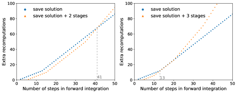
Figure 3: Comparison in terms of recomputations between checkpointing only solutions and checkpointing solutions and stage values. In this example we assume that the memory available at runtime can hold up to $12$ units (one solution or one stage corresponds to one unit). If we save only the solution at a time step, $12$ checkpoints can be used. Saving one solution and two stages results in $4$ checkpoints available, and saving one solution and three stages leads to $3$ checkpoints.

5 Examples

This section presents three representative examples from a diverse set of problems. The goals are to (1) illustrate the use of the PETSc TSAdjoint in outer-loop applications such as optimal control and inverse problems, (2) demonstrate the efficiency and scalability of the implementation, and (3) show the usability of PETSc TSAdjoint in other scientific computing libraries. To date, TSAdjoint has been applied in domains including power systems [39], data assimilation [9], and computational fluid dynamics [25]. These applications are not covered in this paper. We refer readers to these references for more information.

5.1 An optimal control problem

The goal of aircraft trajectory planning is to find a control sequence that can control the pursuer to the targeting leader by minimizing a given cost function, as illustrated in Figure 4(a). The sequence is divided into finite time intervals $T_{k}=[t_{k},t_{k+1}]$ for $k=0,1,\dots,N-1$. In each interval, control inputs are provided in response to the changes in the leader’s position. The dynamics of the aircraft is governed by a nonlinear kinematic model

(33) $$\dot{x}_{k}(t)=v_{k}(t)\cos(\omega_{k}(t))$$

$$\dot{y}_{k}(t)=v_{k}(t)\sin(\omega_{k}(t))$$

defined on each time interval $T_{k}$.

The problem can be transformed into the minimization of the cost function

(34) $$\psi(\bm{u},\bm{p})=\int_{0}^{t_{F}}\|\bm{u}(t)-\bm{u}_{\texttt{leader}}(t)\|^{2}dt,\ \bm{u}=[x(t),y(t)]^{T},\ \bm{p}=[v(t),\omega(t)]^{T}$$

subject to dynamical constraints (33) and inequality constraints

(35) $$v_{\texttt{min}}\leq v(t)\leq v_{\texttt{max}},\quad\omega_{\texttt{min}}\leq\omega(t)\leq\omega_{\texttt{max}}.$$

This is a simple example from [30] but has all the complexities including nonlinearity and inequality constraints that are common for practical dynamical optimal control applications. We implemented this example in PETSc using PETSc time integrators for solving the dynamical system and using TAO for optimization. For optimization, we use the exact Newton method and the classic limited-memory Broyden–Fletcher–Goldfarb–Shanno (BFGS) method in TAO. The first-order derivative information (that is, the gradient $\nabla_{\bm{p}}\psi$) required by both methods is obtained with the first-order adjoint solver, while the second-order derivative information required by the exact Newton method is obtained with the second-order adjoint solver and provided in a matrix-free form (as the Hessian-vector product $\nabla^{2}_{\bm{p}}\psi\,\bm{\sigma}$). The bound constraints are handled by using an active-set approach [12, 13] in which the problem is reduced to an unconstrained minimization problem and the descent direction is searched by the projected line search.

Figure 4(b) shows that the second-order derivative calculated with the PETSc adjoint solver speeds up the convergence of the optimization significantly: the exact Newton method takes $7$ iterations to drive the norm of the gradient of the objective function below $10^{-13}$, whereas the BFGS method [7] approaches $10^{-8}$ after $50$ iterations.

(a) Trajectory of the leader (red) and candidate trajectories of the pursuer (blue).

(b) Convergence of the optimization methods.

Figure 4: Aircraft trajectory planning: (a) schematic of the problem and (b) comparison in convergence between the limited-memory BFGS method and the Newton method with the exact Hessian in matrix-free form.

To validate the gradient computed with the adjoint solver, we leverage the feature of automatically comparing the gradient with the finite-difference approximation in TAO, and we perform a analogous test of the Taylor remainder convergence test in [15]. While the comparison itself can indicate the quality of the adjoint solution, the convergence test shows the consistency between the forward model and the adjoint model. By observing that

(36a) $$\psi(\bm{u},\bm{p}+h\tilde{\bm{p}})-\psi(\bm{u},\bm{p})\rightarrow 0\text{ with }\mathcal{O}(h)\,,~{}\textnormal{and}$$

(36b) $$\psi(\bm{u},\bm{p}+h\tilde{\bm{p}})-\psi(\bm{u},\bm{p})-h\tilde{\bm{p}}\nabla_{\bm{p}}\psi\rightarrow 0\text{ with }\mathcal{O}(h^{2}),$$

we find that the difference between the gradient approximated by using central finite-difference and the adjoint solution converges at second order:

(37) $$\|\nabla_{\bm{p}}\widetilde{\psi}-\nabla_{\bm{p}}\psi\|\rightarrow 0\text{ at }\mathcal{O}(h^{2}).$$

Table 2 shows the results of the convergence test. As expected, a second-order convergence is achieved, indicating that the adjoint solution is correct.

Table 2: Convergence test for the gradient computed with TSAdjoint. It is performed for the first gradient calculation in the optimization loop. RK4 is used for time integration.

h	$\|\nabla_{p}\psi-\widetilde{\nabla}_{p}\psi\|$	order
0.005	3.415e-6
0.0005	3.416e-8	2
0.00005	3.334e-10	2

5.2 An inverse initial value problem

This example demonstrates the application of adjoint methods in an inverse problem of recovering the initial condition for a time-dependent PDE and illustrates the parallel performance of the adjoint calculation involved. The problem can be formulated as a PDE-constrained optimization problem that minimizes the $L_{2}$ norm of the discrepancy between simulated and observed results:

(38) $$\mathop{\text{minimize}}_{\bm{U}_{0}}\|\bm{U}(t_{f})-\bm{U}^{ob}(t_{f})\|^{2}$$

subject to the Gray–Scott equations [22]

(39) $$\dot{\mathbf{u}}=D_{1}\nabla^{2}\mathbf{u}-\mathbf{u}\mathbf{v}^{2}+\gamma\,(1-\mathbf{u})$$

$$\dot{\mathbf{v}}=D_{2}\nabla^{2}\mathbf{v}+\mathbf{u}\mathbf{v}^{2}-(\gamma+\kappa)\,\mathbf{v},$$

where $\bm{U}=[\mathbf{u}\,\mathbf{v}]^{T}$ is the PDE solution vector and $\bm{U}_{0}$ is the initial condition. The PDE models the reaction and diffusion of two interacting species that produce spatial patterns over time, as shown in Figure 5.

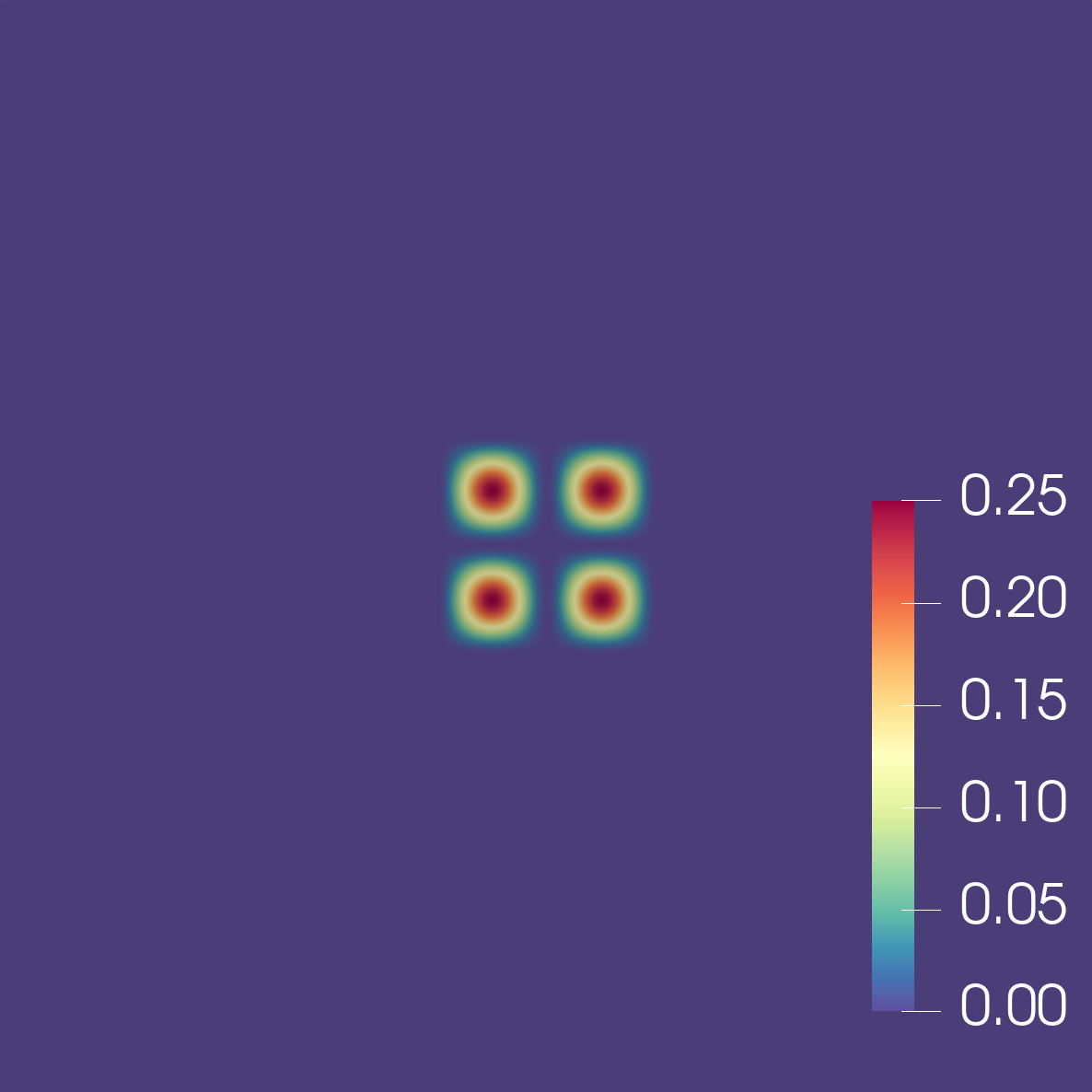
(a) t=0 sec

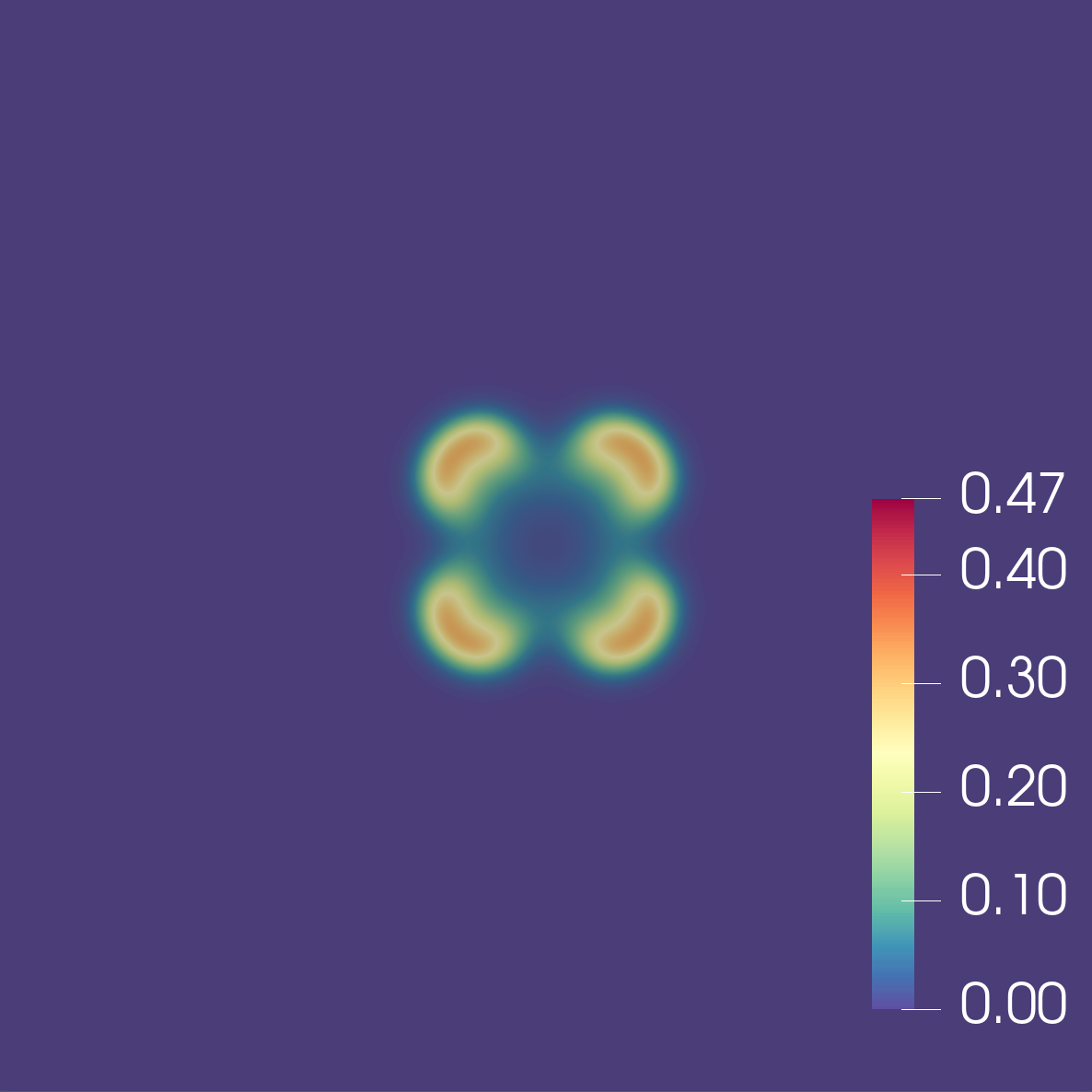
(b) t=100 sec

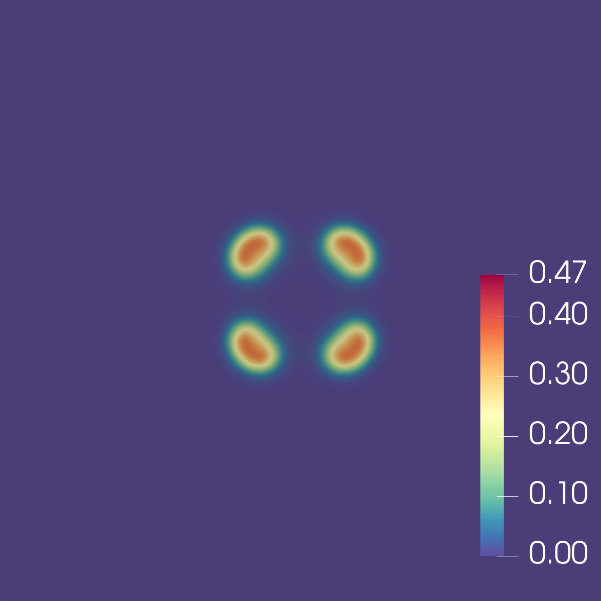
(c) t=200 sec

Figure 5: Evolving spatial patterns of the concentrations $v$ in the Gray–Scott equations.

In our simulation, the PDE is solved with the method of lines. A centered finite-difference scheme is used for spatial discretization. The computational domain is $\Omega\subset[0,2]^{2}$. The time interval is $[t_{0},t_{f}]=[0,5]$. A reference solution is generated from the initial condition

(40) $$\mathbf{u}_{0}=1-2\mathbf{v}_{0},\quad\mathbf{v}_{0}=\begin{cases}\sin^{2}{(4\pi x})\cos^{2}{(4\pi y)}/4,\;\forall x,y\in[1.0,1.5]\\ 0\;\text{otherwise}\end{cases}$$

and set as observed data. The nonlinear system that arises at each time step is solved by using a Newton-based method with line search. For large-scale experiments, we use the geometric algebraic multigrid (GAMG) preconditioner with the following options:

⬇

-mg_levels_ksp_type richardson -mg_levels_pc_type jacobi

-pc_gamg_process_eq_limit 500 -pc_gamg_square_graph 10

-pc_gamg_reuse_interpolation -pc_gamg_repartition false

The last two options allow us to reuse the prolongation operator and avoid repartitioning across the iterations, thus mitigating the performance impact of the setup phase, which is complex and difficult to scale for algebraic multigrid preconditioners [5].

To solve the optimization problem, we use the limited-memory BFGS algorithm [7] in TAO [13] by providing to TAO a function that returns the value of the objective function and its gradient with respect to $U_{0}$ in the Euclidean space (thus implying mesh dependence [32]). The function is computed with a forward solve solving the PDE for solution and evaluation of the objective function, followed by an adjoint solve calculating the gradient expressed by (30). The gradient is verified by using an analog of the Taylor convergence test described in Section 5.1. As shown in Table 3, the theoretical order of convergence $2$ is achieved, indicating that the adjoint solution is correct.

Table 3: Convergence test for the gradient computed with TSAdjoint. It is performed for the first gradient calculation in the optimization loop. The grid size is set to $50\times 50$. RK4 is used for time integration.

h	$\|\nabla_{\bm{U}_{0}}\psi-\nabla_{\bm{U}_{0}}\widetilde{\psi}\|$	order
0.005	2.649e-3
0.0005	2.648e-5	2
0.00005	2.649e-7	2

Efficiency The efficiency of the adjoint solver can be defined by the ratio of the cost of the forward solve to the cost of the adjoint solve. The results for three timestepping methods are presented in Table 4.

Table 4: Performance comparison of two different Jacobian evaluation strategies and three selected timestepping methods. The grid size used in the tests is $100\times 100$. A fixed stepsize of $0.5$ is used on the time interval $[0,5]$.

Jacobian	Time integration	Wall time (second)	Ratio (adjoint/forward)	Iterations	First-order computations	RHS evaluations	Jacobian evaluations
Analytical	Backward Euler	30.0	0.48	188	194	5,870	5,870
	Crank–Nicolson	45.4	0.76	253	264	10,581	10,581
	Runge–Kutta 4	25.6	38.03	246	253	10,120	10,120
FDColoring	Backward Euler	19.9	0.48	188	196	67,190	-
	Crank–Nicolson	28.8	0.66	246	254	127,252	-
	Runge–Kutta 4	11.8	16.48	244	255	122,400	-
Matrix-free	Backward Euler	4.3	0.40	186	194	5,869	-
	Crank–Nicolson	5.1	0.41	240	246	9,865	-
	Runge–Kutta 4	1.8	1.11	229	237	9,480	-

The two selected implicit methods, backward Euler and Crank–Nicolson, are special cases of the theta method ($\theta=1/2$ for backward Euler and $\theta=0$ for Crank–Nicolson). Both achieve an efficiency ratio of less than $1$. For linear problems, the optimal ratio is $1$, assuming the cost of assembling the linear system and the right-hand side is identical and the cost of solving the transposed linear system in an adjoint time step is equivalent to the cost of solving the system in the corresponding forward time step. For nonlinear problems, a smaller ratio is expected because the forward solve requires the solution of one or more (depending on the timestepping algorithm) nonlinear systems while the adjoint run requires only the solution of linear systems at each adjoint time step, the number of which is the same as the number of nonlinear systems required in the forward time step. In this example, the nonlinear solve takes $2$ Newton iterations on average. The adjoint solver based on the backward Euler scheme is slightly more efficient than the adjoint solver based on the Crank–Nicolson scheme because the Jacobian evaluation needed in equation (14b) can be avoided for backward Euler when the mass matrix is the identity. This kind of performance optimization can be discovered easily from the formula and implemented; however, it is difficult to be realized by algorithmic differentiation tools.

The fourth-order explicit method, Runge–Kutta 4, has a relatively high efficiency ratio when using the explicit Jacobian, mainly because the right-hand side evaluation is significantly faster than the Jacobian evaluation, which consists of costly memory operations including assembling the matrix. When using the matrix-free approach, however, the efficiency ratio is significantly improved for Runge–Kutta 4, while the ratios for the other two methods tested within PETSc are slightly improved.

Interestingly, using finite differences and coloring outperforms the analytical Jacobian for this example and implementation. As Table 4 indicates, the number of iterations of the optimization process does not vary much between the two choices. The Jacobian approximation takes $10$ right-hand side function evaluations ($5$ colors and 2 components in the PDE). Although finite differences need more arithmetic operations, the array of values generated from the approximation can be transferred into a PETSc sparse matrix efficiently. In contrast, in the implementation of the analytical Jacobian, the matrix values are set row-wise, which is natural for sparse matrices in the compressed sparse row format but less cache-efficient.

Parallel scaling. To demonstrate the scalability of the adjoint solver, we ran the gradient calculation portion of this benchmark problem with fine grid resolution on the Intel Xeon Phi Knights Landing (KNL) nodes of the NERSC supercomputer Cori. Each KNL node is assigned $64$ MPI processes with one process per core. Manually optimized linear algebra kernels (e.g., vectorized matrix-vector multiplication [40]) are used for the best performance. Figure 6 shows the scaling results for up to $8,192$ MPI processes. Backward Euler and Crank–Nicolson exhibit good parallel scaling for both the forward solve and the adjoint solve. In fact, the solve phase of GAMG scales well in the strong-scaling regime. The setup phase scales up to $40,96$ processes. For Runge–Kutta 4, the scaling of the forward solve is not ideal because the communication cost in the right-hand side function becomes relatively large compared with the computation time as the number of processes increases. For the adjoint solve, however, perfect linear scaling is observed.

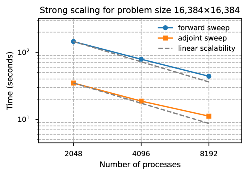
(a) Backward Euler

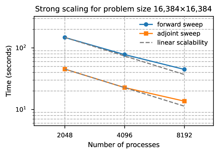
(b) Crank–Nicolson

(c) Runge–Kutta 4

Figure 6: Strong scaling of the adjoint sensitivity calculation for the 2D reaction-diffusion equation (39) on NERSC’s supercomputer Cori. In all the tests, $32$, $64$, and $128$ compute nodes with $64$ MPI processes on each node are used. The grid size is $16,384\times 16,384$ (yielding about $0.5$ billion degrees of freedom). Three time integrations methods are tested.

5.3 A Firedrake example: adjoint of Burgers’ equation

We consider Burgers’ equation on a uniform square mesh:

(41) $$\dot{\bm{U}}+(\bm{U}\cdot\nabla)\bm{U}-\nu\Delta\bm{U}=0$$

$$(n\cdot\nabla)\bm{U}=0\ \textrm{on}\ \Omega,$$

where $\Omega$ is the domain and $\nu$ is a constant scalar viscosity. The equation is discretized in space by using Lagrange finite elements of polynomial degree 2. The initial condition is a Gaussian profile with amplitude $1.0$ and distribution width $0.06$, as shown in Figure 7; and $16$ uniform time steps are used on the time interval $[0,2]$ seconds. For testing, we compute the sensitivity of the $H^{1}$ error norm of the solution in the finite-element function space with respect to the initial condition:

(42) $$\int_{\Omega}\left((\bm{U}-\bm{U}_{r})\cdot(\bm{U}-\bm{U}_{r})+(\nabla\bm{U}-\nabla\bm{U}_{r})\cdot(\nabla\bm{U}-\nabla\bm{U}_{r})\right)\mathrm{d}x,$$

where the reference solution $\bm{U}_{r}$ is computed by using a strict stepsize and a fine mesh. This example is implemented by using only a few lines of Python code. The right-hand side function and Jacobian function defining the ODE problem are automatically generated by specifying the variational formulations of the semi-discretized PDE using Firedrake; they are provided to the PETSc timestepping solver through petsc4py [11] for the forward and the adjoint solution.

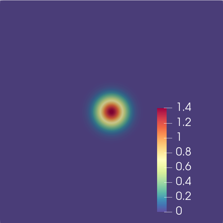
(a)

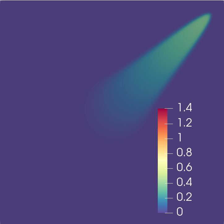
(b)

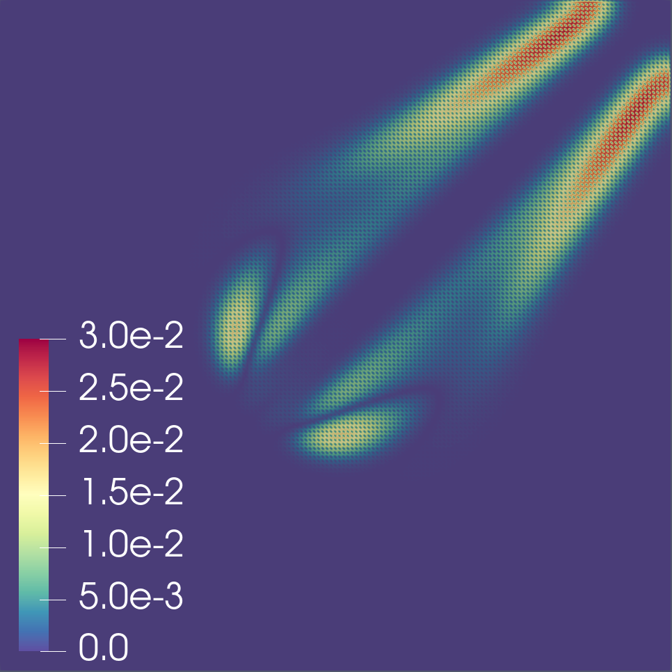
(c)

Figure 7: Initial condition (a), final solution at $T=2s$ (b), and sensitivity of the $H^{1}$ error norm with respect to the initial condition in the Lagrangian function space (c).

Table 5 lists the total runtime and number of right-hand side and Jacobian evaluations for both the forward and the adjoint computation. We observe that the adjoint-to-forward ratios are $0.25$ for backward Euler and $0.14$ for Crank–Nicolson. While the runtime of the forward solve differs significantly for the time integration methods, the runtime of the adjoint solve is approximately the same. The reason is that the right-hand side function evaluation (the spatial discretization) dominates the total computational cost, while the adjoint solver of backward Euler or Crank–Nicolson requires the same number of Jacobian evaluations and the same number of linear solves (one per adjoint time step).

Table 5: Timings of Burgers’ adjoint in Firedrake.

Time integration	Stage	Wall time (second)	Ratio	RHS evaluations	Jacobian evaluations
Backward Euler	forward run	22.386	1	142	109
	reverse run	5.543	0.25	0	32
Crank–Nicolson	forward run	40.704	1	254	157
	reverse run	5.868	0.14	0	32

6 Conclusion

Algorithmic differentiation has long been needed by many scientific applications, especially as machine learning becomes increasingly popular. It has been realized at different abstraction levels, posing different challenges for application developers and software developers. The new tool presented in this paper, PETSc TSAdjoint, provides an efficient and accurate approach for computing first-order and second-order adjoints for ODEs, DAEs, and time-dependent nonlinear PDEs. It makes the task of gradient calculation easier by avoiding full differentiation of the entire code, with no loss of accuracy and speed. Minimal changes are required for applications using PETSc time integrators to be equipped with sensitivity analysis capabilities. An optimal checkpointing component has been developed to deliver transparent and optimal checkpointing strategies on high-performance computing platforms. Parallelism is inherited from PETSc parallel infrastructures. Thanks to the hierarchical structure of PETSc, the adjoint solvers take advantage of the well-developed nonlinear and linear iterative solvers and the extensive collection of preconditioners in PETSc.

Extensive experiments have been performed to demonstrate the usability, efficiency, and scalability of the adjoint solvers. We have shown that they can be easily used with various other scientific computing libraries or tools in different programming languages. We have also shown that using finite differences and coloring and relying on high-level AD are efficient and convenient alternatives to deriving and implementing an analytical Jacobian. For first-order adjoints, the adjoint solve cost is typically less than the forward solve cost when implicit timestepping methods are employed. The performance ratio for explicit methods can exceed 1 if the Jacobian matrix is provided in the explicit form; however, this could be mitigated by using matrix-free implementations. Furthermore, the adjoint computation of PDEs scales nicely to large numbers of cores on a supercomputer, even when the scaling of the forward solve is not ideal. In addition, we show how the second-order adjoint sensitivities can be used to accelerate the convergence of optimization in an optimal control problem. Without a doubt, Hessian-related information for the dynamical system is needed by second-order adjoints and may be difficult to compute. However, PETSc TSAdjoint requires only a rank-1 vector-Hessian-vector product for the second-order adjoints.

As far as we know, this library is the first general-purpose HPC-friendly library that offers first-order and second-order discrete adjoint capabilities based on multistage time integration methods, supports sensitivity analysis for hybrid dynamical systems, and comes with sophisticated checkpointing support that is transparent to users. We expect that more applications in PDE-constrained optimization, data assimilation, uncertainty quantification, and machine learning will be enabled by our development.

References

- [1] S. Abhyankar, J. Brown, E. M. Constantinescu, D. Ghosh, B. F. Smith, and H. Zhang, PETSc/TS: a modern scalable ODE/DAE solver library, arXiv e-preprints, (2018), https://arxiv.org/abs/1806.01437.
- [2] M. Alexe and A. Sandu, On the discrete adjoints of adaptive time stepping algorithms, Journal of Computational and Applied Mathematics, 233 (2009), pp. 1005–1020, https://doi.org/https://doi.org/10.1016/j.cam.2009.08.109.
- [3] M. S. Alnaes, J. Blechta, A. J. J. Hake, B. Kehlet, A. Logg, C. Richardson, J. Ring, M. E. Rognes, and G. N. Wells, The FEniCS Project Version 1.5, Archive of Numerical Software, (2015), https://doi.org/10.11588/ans.2015.100.20553.
- [4] J. A. E. Andersson, J. Gillis, G. Horn, J. B. Rawlings, and M. Diehl, CasADi – A software framework for nonlinear optimization and optimal control, Mathematical Programming Computation, 11 (2019), pp. 1–36.
- [5] A. H. Baker, T. Gamblin, M. Schulz, and U. M. Yang, Challenges of scaling algebraic multigrid across modern multicore architectures, in 2011 IEEE International Parallel Distributed Processing Symposium, 2011, pp. 275–286, https://doi.org/10.1109/IPDPS.2011.35.
- [6] R. A. Bartlett, D. M. Gay, and E. T. Phipps, Automatic differentiation of c++ codes for large-scale scientific computing, in Computational Science – ICCS 2006, V. N. Alexandrov, G. D. van Albada, P. M. A. Sloot, and J. Dongarra, eds., Berlin, Heidelberg, 2006, Springer Berlin Heidelberg, pp. 525–532.
- [7] S. J. Benson and J. J. More, A limited memory variable metric method in subspaces and bound constrained optimization problems, tech. report, in Subspaces and Bound Constrained Optimization Problems, 2001.
- [8] C. H. Bischof, L. Roh, and A. J. Mauer-Oats, ADIC: An extensible automatic differentiation tool for ANSI-C, Software - Practice and Experience, 27 (1997), pp. 1427–1454, https://doi.org/10.1002/(SICI)1097-024X(199712)27:12<1427::AID-SPE138>3.0.CO;2-Q.
- [9] L. Carracciuolo, E. M. Constantinescu, and L. D’Amore, Validation of a PETSc based software implementing a 4DVAR data assimilation algorithm: a case study related with an oceanic model based on shallow water equation, arXiv e-prints, (2018), https://arxiv.org/abs/1810.01361.
- [10] E. M. Constantinescu, Generalizing global error estimation for ordinary differential equations by using coupled time-stepping methods, Journal of Computational and Applied Mathematics, 332 (2018), pp. 140–158, https://doi.org/https://doi.org/10.1016/j.cam.2017.05.012.
- [11] L. D. Dalcin, R. R. Paz, P. A. Kler, and A. Cosimo, Parallel distributed computing using Python, Advances in Water Resources, 34 (2011), pp. 1124–1139, https://doi.org/10.1016/j.advwatres.2011.04.013.
- [12] A. Dener, A. Denchfield, T. Munson, J. Sarich, S. Wild, S. Benson, and L. C. McInnes, Tao users manual, Tech. Report ANL/MCS-TM-322 - Revision 3.13, Argonne National Laboratory, 2020, https://www.mcs.anl.gov/petsc.
- [13] A. Dener and T. Munson, Accelerating limited-memory quasi-newton convergence for large-scale optimization, in Computational Science – ICCS 2019, vol. 11538 of Lecture Notes in Computer Science, Cham, 2019, Springer International Publishing, pp. 495–507.
- [14] J. Dormand and P. Prince, A family of embedded Runge-Kutta formulae, Journal of Computational and Applied Mathematics, 6 (1980), pp. 19–26, https://doi.org/https://doi.org/10.1016/0771-050X(80)90013-3.
- [15] P. E. Farrell, D. A. Ham, S. F. Funke, and M. E. Rognes, Automated derivation of the adjoint of high-level transient finite element programs, SIAM Journal on Scientific Computing, 35 (2013), pp. 369–393, https://doi.org/10.1137/120873558.
- [16] A. H. Gebremedhin, F. Manne, and A. Pothen, What color is your Jacobian? Graph coloring for computing derivatives, SIAM Review, 47 (2005), pp. 629–705, https://doi.org/10.1137/S0036144504444711.
- [17] A. Gholami, K. Keutzer, and G. Biros, ANODE: Unconditionally accurate memory-efficient gradients for neural ODEs, IJCAI International Joint Conference on Artificial Intelligence, 2019-August (2019), pp. 730–736, https://doi.org/10.24963/ijcai.2019/103, https://arxiv.org/abs/1902.10298.
- [18] R. Giering and T. Kaminski, Recipes for adjoint code construction, ACM Transactions on Mathematical Software, 24 (1998), pp. 437–474, https://doi.org/10.1145/293686.293695.
- [19] A. Griewank and A. Walther, Algorithm 799: revolve: an implementation of checkpointing for the reverse or adjoint mode of computational differentiation, ACM Transactions on Mathematical Software, 26 (2000), pp. 19–45, https://doi.org/10.1145/347837.347846.
- [20] V. Heuveline and A. Walther, Online checkpointing for parallel adjoint computation in PDEs: application to goal-oriented adaptivity and flow control, in Euro-Par 2006, vol. 4128 of Lecture Notes in Computer Science, Springer Berlin Heidelberg, 2006.
- [21] A. C. Hindmarsh, P. N. Brown, K. E. Grant, S. L. Lee, R. Serban, D. E. Shumaker, and C. S. Woodward, SUNDIALS: Suite of nonlinear and differential/algebraic equation solvers, ACM Transactions on Mathematical Software, 31 (2005), pp. 363–396, https://doi.org/10.1145/1089014.1089020.
- [22] W. Hundsdorfer and J. Verwer, Numerical Solution of Time-Dependent Advection-Diffusion-Reaction Equations, Springer Series in Computational Mathematics, Springer Berlin Heidelberg, 2007.
- [23] A. Jameson, Aerodynamic design via control theory, Journal of Scientific Computing, 3 (1988), https://doi.org/10.1007/BF01061285.
- [24] M. Lubin and I. Dunning, Computing in operations research Using Julia, INFORMS Journal on Computing, 27 (2015), pp. 238–248, https://doi.org/10.1287/ijoc.2014.0623.
- [25] O. Marin, E. Constantinescu, and B. Smith, Unsteady PDE-constrained optimization with spectral elements using PETSc and TAO, arXiv e-prints, (2018), https://arxiv.org/abs/1806.01422.
- [26] D. Onken and L. Ruthotto, Discretize-Optimize vs. Optimize-Discretize for Time-Series Regression and Continuous Normalizing Flows, (2020), http://arxiv.org/abs/2005.13420, https://arxiv.org/abs/2005.13420.
- [27] A. Paszke, S. Chintala, G. Chanan, Z. Lin, S. Gross, E. Yang, L. Antiga, Z. Devito, A. Lerer, and A. Desmaison, Automatic differentiation in PyTorch, 31st Conference on Neural Information Processing Systems, (2017), https://doi.org/10.1017/CBO9781107707221.009, https://arxiv.org/abs/arXiv:1011.1669v3.
- [28] C. Rackauckas, Y. Ma, V. Dixit, X. Guo, M. Innes, J. Revels, J. Nyberg, and V. Ivaturi, A comparison of automatic differentiation and continuous sensitivity analysis for derivatives of differential equation solutions, arXiv preprint arXiv:1812.01892, (2018).
- [29] C. Rackauckas and Q. Nie, Differentialequations. jl–a performant and feature-rich ecosystem for solving differential equations in julia, Journal of Open Research Software, 5 (2017).
- [30] R. Raffard and C. Tomlin, Second order adjoint-based optimization of ordinary and partial differential equations with application to air traffic flow, Proceedings of the 2005, American Control Conference, (2005), pp. 798–803, https://doi.org/10.1109/ACC.2005.1470057.
- [31] F. Rathgeber, D. A. Ham, L. Mitchell, M. Lange, F. Luporini, A. T. T. Mcrae, G.-T. Bercea, G. R. Markall, and P. H. J. Kelly, Firedrake: Automating the finite element method by composing abstractions, ACM Transactions on Mathematical Software, 43 (2016), pp. 24:1–24:27, https://doi.org/10.1145/2998441, http://doi.acm.org/10.1145/2998441.
- [32] T. Schwedes, D. A. Ham, S. W. Funke, M. D. Piggott, T. Schwedes, D. A. Ham, S. W. Funke, and M. D. Piggott, Mesh dependence in PDE-constrained optimisation, in Mesh Dependence in PDE-Constrained Optimisation, 2017, https://doi.org/10.1007/978-3-319-59483-5_2.
- [33] G. Söderlind, Digital filters in adaptive time-stepping, ACM Transactions on Mathematical Software, 29 (2003), pp. 1–26, https://doi.org/10.1145/641876.641877.
- [34] P. Stumm and A. Walther, MultiStage approaches for optimal offline checkpointing, SIAM Journal on Scientific Computing, 31 (2009), pp. 1946–1967, https://doi.org/10.1137/080718036.
- [35] P. Stumm and A. Walther, New algorithms for optimal online checkpointing, SIAM Journal on Scientific Computing, 32 (2010), pp. 836–854.
- [36] J. G. Wallwork, P. Hovland, H. Zhang, and O. Marin, Computing derivatives for PETSc adjoint solvers using algorithmic differentiation, arXiv e-prints, (2019), https://arxiv.org/abs/1909.02836.
- [37] A. Walther and A. Griewank, Getting started with ADOL-C, in Combinatorial Scientific Computing, Chapman-Hall CRC Computational Science, 2012, pp. 181–202, https://doi.org/10.1201/b11644-8.
- [38] Q. Wang, P. Moin, and G. Iaccarino, Minimal repetition dynamic checkpointing algorithm for unsteady adjoint calculation, SIAM Journal on Scientific Computing, 31 (2009), pp. 2549–2567, https://doi.org/10.1137/080727890.
- [39] H. Zhang, S. Abhyankar, E. Constantinescu, and M. Anitescu, Discrete adjoint sensitivity analysis of hybrid dynamical systems with switching, IEEE Transactions on Circuits and Systems I: Regular Papers, 64 (2017), pp. 1247–1259, https://doi.org/10.1109/TCSI.2017.2651683.
- [40] H. Zhang, R. T. Mills, K. Rupp, and B. F. Smith, Vectorized parallel sparse matrix-vector multiplication in PETSc using AVX-512, in Proceedings of the 47th International Conference on Parallel Processing - ICPP 2018, ACM Press, 2018, pp. 1–10, https://doi.org/10.1145/3225058.3225100.
- [41] H. Zhang and A. Sandu, FATODE: a library for forward, adjoint, and tangent linear integration of ODEs, SIAM Journal on Scientific Computing, 36 (2014), pp. C504–C523, https://doi.org/10.1137/130912335.