Higgs-Squark-Slepton Inflation from the MSSM

Abstract

The inflation within the MSSM is proposed, where the inflaton field is a combination of the Higgs, squark and slepton states. While the inflationary phase is fully governed by the electron Yukawa superpotential coupling, the fields’ condensates float along the flat $D$-term trajectory. This predicts the MSSM parameter $\tan\beta\simeq 13.1$ determined via the value of the curvature perturbation amplitude. The values of the scalar spectral index and the tensor-to-scalar ratio are predicted to be $n_{s}\simeq 0.966$ and $r=0.00118$. The postinflation reheating of the Universe proceeds by the radiative decay of the inflaton to the two gluons ($\phi\to gg$) with the reheating temperature $T_{r}\simeq 1.4\cdot 10^{7}$ GeV.

I I. Introduction

Besides the firm support from the Planck Collaboration measurements Akrami:2018odb , the inflationary paradigm first-infl has strong theoretical motivations. It elegantly solves many problems of the big bang cosmology. It is very motivated and also, as it turns out, highly challenging to build successful inflation which has close connection to the particle physics model whith consistent construction. For this purpose, the supersymmetric (SUSY) setup (insuring flatness of the inflaton’s potentiol protected by the supersymmetry) looks one of the best choice susy-infl and the Standard Model’s minimal SUSY extension (MSSM) seems the reasonable framework to deal with. However, most of the successful inflation models exploit additional MSSM singlet(s). Among those are models of inflation within NMSSM framework NMSSM-infl , which although motivated by theoretical and phenomenological reasons, have reduced predictive power because of additional parameters. Inflation models with MSSM field content exploiting slepton and/or squark states along $D$-term flat directions has been studied in numerous works Allahverdi:2006iq but with utilizing higher order operators involving new free parameters in the inflation process. Note that the successful inflation within various well motivated extensions of the MSSM, such as SUSY GUTs and SUSY left-right symmetric models, have been considered GUT-infl . However, still, all these constructions involve additional MSSM singlet states with additional couplings.

In a recent paper Tavartkiladze:2019cfb within the MSSM, the model of inflation along $D$-flat trajectory was proposed, where inflaton field emerged as a combination of the slepton and Higgs fields. The model utilized nonminimal Kähler potential, however, in the inflation and postinflation reheating processes only MSSM Yukawa superpotential couplings have been involved. This made the model very predictive. In this paper we pursue this approach and investigate the possibility of involvement of the squark (the superpartners of the quarks) states into the inflation process. We present an interesting and novel possibility in which inflaton emerges as a superposition of the Higgs, squark and slepton states. The inflaton potential, emerged from the superpotential $F$-term, involves only the electron Yukawa coupling. This fixes the value of the MSSM parameter $\tan\beta$. Besides this, the inflaton decay and subsequent reheating process is fully governed by the known MSSM couplings. Thus, very close interconnection between cosmology and particle physics model is established.

Successful inflation is realized by the specific form of nonminimal Kähler potential. Proposed inflation model, which is disucussed and investigated in next two sections, also has several interesting phenomenological implications (discussed at the end of the paper).

II II. The framework and the inflaton potential

The framework we are using is the $N=1$ supergravity sugra-pot ; Kugo:1982mr . The action is built up from the $D$ and $F$-term Lagrangian densities

$${\cal L}_{D}+{\cal L}_{F}~{},$$ (1)

which are determined by the Kähler potential ${\cal K}$, the superpotential $W$ and by the gauge kinetic function $f_{IJ}$. By the superconformal formulation, the ${\cal L}_{D,F}$ are given as follows Kugo:1982mr :

$${\cal L}_{D}=-3\int\!\!d^{4}\theta\,e^{-{\cal K}/3}\bar{\phi}^{\dagger}\bar{\phi},$$

$${\cal L}_{F}=\int\!\!d^{2}\theta\bar{\phi}^{3}\,W+\frac{1}{4}\int\!\!d^{2}\theta f_{IJ}{{\cal W}}^{\alpha I}{{\cal W}}_{\alpha}^{J}+{\rm h.c.}$$ (2)

where $\bar{\phi}$ is the conformal compensator chiral superfield. The ${{\cal W}}^{\alpha I}$ denote the gauge chiral superfield corresponding to the $SU(3)_{c}$, $SU(2)_{L}$ and $U(1)_{Y}$ symmetries. We will consider $f_{IJ}=\delta_{IJ}$ - the canonical kinetic terms for the gauge superfields. In (2) and below, where it is convenient, we set the reduced Planck mass $M_{Pl}$ to one. In this way, any dimensionful quantity will be understood to be measured in the unit(s) of $M_{Pl}$($=2.4\times 10^{18}$ GeV).

The Kähler potential ${\cal K}$ and the superpotential $W$ are the functions of the MSSM chiral superfields $\Phi_{I}$. The latter are three families of quark and lepton superfields $\left(q,u^{c},d^{c},l,e^{c}\right)_{\alpha}$ ($\alpha=1,2,3$ is the family index), and the up and down-type Higgs doublet chiral superfields $h_{u},h_{d}$:

$$\Phi_{I}=\left\{\left(q,u^{c},d^{c},l,e^{c}\right)_{\alpha},h_{u},h_{d}\right\}.$$ (3)

After integrating out the auxiliary fields and fixing the conformal symmetries $\bar{\phi}=1$, the scalar potential will get contributions from $F$ and $D$-terms:

$$V=V_{F}+V_{D},$$ (4)

where the $F$-term scalar potential is given by sugra-pot ; Kugo:1982mr :

$$V_{F}=\,e^{{\cal K}}\left(D_{\bar{J}}{\bar{W}}{\cal K}^{{\bar{J}}I}D_{I}W-3|W|^{2}\right),$$ (5)

where $D_{I}W\!=\!(\frac{\partial}{\partial\Phi_{I}}+\frac{\partial{\cal K}}{\partial\Phi_{I}})W$ and $D_{\bar{J}}{\bar{W}}\!=\!(\frac{\partial}{\partial\Phi_{J}^{\dagger}}+\frac{\partial{\cal K}}{\partial\Phi_{J}^{\dagger}}){\bar{W}}$. The matrix ${\cal K}^{{\bar{J}}I}$ is an inverse of the Kähler ‘metric’ ${\cal K}_{I{\bar{J}}}=\frac{\partial^{2}{\cal K}}{\partial\Phi_{I}\partial\Phi_{I}^{\dagger}}$. Thus, ${\cal K}_{I{\bar{M}}}{\cal K}^{{\bar{M}}J}=\delta_{I}^{J}$ and ${\cal K}^{{\bar{I}}M}{\cal K}_{M{\bar{J}}}=\delta^{\bar{I}}_{\bar{J}}$.

Further, we will use the following nonminimal Kähler potential:

$${\cal K}=-\ln(1-\sum_{I}\Phi_{I}^{\dagger}e^{-V}\Phi_{I})~{},$$ (6)

which in the small field limit ($\Phi_{I}\!\ll 1$) has the canonical form ${\cal K}\to\sum_{I}\Phi_{I}^{\dagger}e^{-V}\Phi_{I}$. However, for the large values of the fields, as was shown Tavartkiladze:2019cfb , the form of (6) together with the MSSM Yukawa superpotential terms can give successful inflation with observables determined in terms of the MSSM parameters. Note that with logarithmic but slightly different Kähler potential (exploiting MSSM singlet states), the successful chaotic inflation was realized in Refs. Kallosh:2013hoa ; Ferrara:2016fwe . In this paper, we study the inflation with the inflaton emerging from the scalar components of the MSSM states only. We will be focusing to realize inflation along the flat $D$-term trajectory, i.e. $\langle V_{D}\rangle=0$ during the inflation. In works Affleck:1984fy ; Dine:1995kz the slepton and/or squark condensates along the flat directions have been used for the baryogenesis process in the early Universe. The inflation with sleptons and/or squarks has been studied in Refs. Allahverdi:2006iq , however, these constructions exploit higher order operators with many new parameters involved in the inflation process.

With the Kähler potential (6), the $D$-term potential $V_{D}$ is build from the Killing potentials ${\cal D}_{G}$ corresponding to the $U(1)_{Y},SU(2)_{L}$ and $SU(3)_{c}$ gauge symmetries [$G=Y,SU(2),SU(3)$]:

$$V_{D}=\frac{g_{1}^{2}}{8}{\cal D}_{Y}^{2}+\frac{g_{2}^{2}}{2}({\cal D}^{i}_{SU(2)})^{2}+\frac{g_{3}^{2}}{2}({\cal D}^{a}_{SU(3)})^{2}.$$ (7)

The Killing potentials ${\cal D}_{G}$ are related to the $D$-terms as

$${\cal D}_{G}=\frac{D_{G}}{1-\sum_{I}\Phi_{I}^{\dagger}\Phi_{I}}$$ (8)

where $\Phi_{I}$ in (8) stand for lowest scalar component of the corresponding chiral superfield. On the other hand, the $D$-terms $D_{G}$ corresponding to the $U(1)_{Y}$, $SU(2)_{L}$ and $SU(3)_{c}$, are respectively:

$$D_{Y}=|h_{d}|^{2}-|h_{u}|^{2}-2|\tilde{e}^{c}_{\alpha}|^{2}+|\tilde{l}_{\alpha}|^{2}$$

$$-\frac{1}{3}|\tilde{q}_{\alpha}|^{2}+\frac{4}{3}|\tilde{u}^{c}_{\alpha}|^{2}-\frac{2}{3}|\tilde{d}^{c}_{\alpha}|^{2}~{},$$

$$D^{i}_{SU(2)}=\!\frac{1}{2}\!\left(h_{d}^{\dagger}\tau^{i}h_{d}-h_{u}^{\dagger}\tau^{i}h_{u}+\tilde{l}_{\alpha}^{{\dagger}}\tau^{i}\tilde{l}_{\alpha}+\tilde{q}_{\alpha}^{{\dagger}}\tau^{i}\tilde{q}_{\alpha}\right),$$

$$D^{a}_{SU(3)}=\!\frac{1}{2}\!\left(\tilde{q}_{\alpha}^{{\dagger}}\lambda^{a}\tilde{q}_{\alpha}-\tilde{u}_{\alpha}^{c{\dagger}}\lambda^{a}\tilde{u}^{c}_{\alpha}-\tilde{d}_{\alpha}^{c{\dagger}}\lambda^{a}\tilde{d}^{c}_{\alpha}q_{\alpha}\right).$$ (9)

In (II) the summation under the family index $\alpha=1,2,3$ is assumed. $\tau^{i}/2$ and $\lambda^{a}/2$ are respectively $SU(2)_{L}$ and $SU(3)_{c}$ generators ($i=1,2,3$, $a=1,\cdots,8$).

One can readely check that given by (8), (II) the equations

$${\cal K}_{I\bar{J}}(iT^{A})^{I}_{M}\Phi_{M}=i\frac{\partial}{\partial\Phi_{J}^{\dagger}}{\cal D}^{A},$$

$${\cal K}_{I\bar{J}}(iT^{A})_{I}^{M}\Phi_{M}^{\dagger}=i\frac{\partial}{\partial\Phi_{I}}{\cal D}^{A}$$ (10)

are automatically satisfied ($T^{A}$ stand for the generator/charge of the corresponding gauge symmetry). As known from supergravity constructions sugra-gauge , these ensure the consistent supergravity gauge invariance.

II.1 II.1. Choice of Flat $D$-term Direction

In MSSM there are numerous solutions with the $D$-term flat directions, which have been classified in Gherghetta:1995dv . Here we consider one (the $e^{c}lqu^{c}$-type flat direction) involving the scalar component of $h_{d}$, the sleptons $\tilde{e}^{c},\tilde{l}$ and the squarks $\tilde{q},\tilde{u}^{c}$. The state $h_{d}$, different families of sleptons, squarks (of the quantum numbers indicated above) will share vacuum expectation values (VEVs) by appropriate weights. In particular, we will consider the following VEV configuration:

$$\langle\tilde{e}^{c}_{1}\rangle\!=\!z,~{}~{}~{}\!\langle h_{d}\rangle\!=\!\left(\begin{array}[]{c}zc_{\theta}\\ 0\end{array}\right),~{}~{}~{}\!\langle\tilde{l}_{2}\rangle\!=\!\left(\begin{array}[]{c}zs_{\theta}\\ 0\end{array}\right)\!\!\begin{array}[]{c}\\ \!\!{~{}}_{\uparrow}\!\!\\ \vspace{-0.1cm}{~{}}_{\!SU(2)_{L}}\!\!\\ \vspace{0.6cm}{~{}}_{\downarrow}{}\end{array}~{}$$ (19)

$$\begin{array}[]{ccc}&{\begin{array}[]{ccc}&~{}~{}~{}~{}{~{}}_{\leftarrow~{}SU(3)_{c}~{}\rightarrow}&\\ \end{array}}\\ &{\!\langle\tilde{q}_{1}\rangle=\left(\begin{array}[]{ccc}0&~{}~{}0&~{}~{}0\\ 0&~{}~{}0&~{}~{}z\end{array}\right)}\end{array}\!\!\!\!\begin{array}[]{c}\\ {~{}}_{\uparrow}\\ \!{~{}}_{SU(2)_{L}}\!\\ \vspace{0.3cm}{~{}}_{\downarrow}{}\end{array}~{}$$ (29)

$$\langle\tilde{u}^{c}\rangle=\!\left(\begin{array}[]{ccc}0,&~{}0,&~{}zc_{\varphi}\end{array}\!\right),~{}~{}~{}~{}~{}$$ (31)

$$\langle\tilde{t}^{c}\rangle=\!\left(\begin{array}[]{ccc}\!0,&0,&zs_{\varphi}e^{i\omega}\!\end{array}\!\right),~{}~{}~{}~{}~{}$$ (33)

where actions of $SU(3)_{c}$ and $SU(2)_{L}$ are depicted schematically. Also, the short handed definitions $\cos(\theta,\varphi)\equiv c_{\theta,\varphi}$ and $\sin(\theta,\varphi)\equiv s_{\theta,\varphi}$ are used. The angles $\theta,\varphi$ and the phase $\omega$ will be determined/fixed from the superpotential. Essential point is the fact that with (33) configuration (and with zero VEVs of all remaining fields), all $D$-terms [of Eq. (II)] vanish (and thus $\langle V_{D}\rangle=0$) for arbitrary values of $z$, $\theta,\varphi$ and $\omega$. While the values of $\theta,\varphi,\omega$ will be fixed, the $z$ will be a dynamical variable and will be related to the inflaton field. As will be shown, this will lead to the predictive and successful inflation. To see how things work out, we need to consider the superpotential couplings.

II.2 II.2. The Superpotential and Inflaton Potential

The MSSM superpotential includes three $Y_{E},Y_{D}$ and $Y_{U}$ Yukawa matrix-couplings and the $\mu$-term:

$$W_{\rm MSSM}\!=\!e^{c}Y_{E}lh_{d}+qY_{D}d^{c}h_{d}+qY_{U}u^{c}h_{u}+\mu h_{u}h_{d}.~{}~{}~{}~{}$$ (34)

Without loss of any generality, we choose the field basis such that the Yukawa matrices are:

$$Y_{E}=Y_{E}^{\rm Diag}={\rm Diag}\left(\lambda_{e},\lambda_{\mu},\lambda_{\tau}\right),$$

$$Y_{D}=Y_{D}^{\rm Diag},~{}Y_{U}=V_{CKM}^{T}Y_{U}^{\rm Diag}.$$ (35)

From Eq. (34), with (33) we have:

$$F_{e^{-}}^{*}=-\lambda_{e}z^{2}c_{\theta}~{}.$$ (36)

In our construction, this will be the only nonvanishing $F$-term contributing to the inflation potential. As mentioned, the $\theta,\varphi$ and $\omega$ will be fixed from the superpotential couplings by imposing the vanishing conditions for all remaining $F$-terms. For instance, the requirement $F_{h_{u}^{(2)}}=0$ gives the condition $z^{2}\left(V_{ud}\lambda_{u}c_{\varphi}+V_{td}e^{i\omega}\lambda_{t}s_{\varphi}\right)=0$, which is satisfied by fixing $\omega$ and $\varphi$ as follows: $\omega=\pi+{\rm Arg}\left(\frac{V_{ud}}{V_{td}}\right)$, $\tan\varphi\!=\!\frac{\lambda_{u}}{\lambda_{t}}\left|\frac{V_{ud}}{V_{td}}\right|\simeq 3\cdot 10^{-4}$ phi-val . Here and below, the $\mu$-term being too small($\sim$few TeV) and therefore irrelevant for inflation, will be ignored. Moreover, we include additional superpotential $W^{\prime}$, which ensures fulfilment of the condition $F_{d^{c}}=0$. Two cases - (i) and (ii) - can be considered which have different low energy implications, but lead to the same inflation process.

(i) $W^{\prime}=-\lambda q_{1}l_{2}d^{c}$. This coupling, together with the couplings (34) gives $\langle F_{d^{c}}^{*}\rangle=z^{2}(-\lambda_{d}c_{\theta}+\lambda s_{\theta})=0$, i.e. fixing the angle $\theta$ as $\tan\theta=\frac{\lambda_{d}}{\lambda}$.

(ii) $W^{\prime}=\lambda e^{c}_{1}(q_{1}l_{2}u^{c})(q_{1}h_{d}d^{c})$ which gives $\langle F_{d^{c}}^{*}\rangle=z^{2}c_{\theta}(-\lambda_{d}+\lambda z^{4}c_{\varphi}s_{\theta})=0$ and fixes the angle $\theta$ as follows $s_{\theta}\simeq\frac{\lambda_{d}}{\lambda z^{4}}$.

For both these cases we will be considering the suppressed values of $\theta<0.1$ (i.e. $c_{\theta}\simeq 1$), therefore expressions given above are pretty accurate te-approx .

It is essential and very important that the values of $\theta,\varphi$ and $\omega$ are fixed. Since they are parameterizing the field configuraation along the $D$-term flat direction [see Eq. (33)] they are dynamical degrees and their fixation means their stabilization. This ensures that during the inflation there are no unstable/runaway directions. Plots in Fig.1 represent the potential as a function of $(\phi,~{}\theta)$ and $(\phi,~{}\varphi)$ variables respectively [$\phi$ denotes inflaton and is related to $z$ via Eq. (47). See also the caption of Fig.1]. They demonstrate that the valley (with a slight slope) is along the direction of the inflaton field $\phi$. Also, it is important that there are no other tachyonic or fast moving degrees of freedom. We have checked, with the couplings and arrangements given above, and made sure that the presented inflation scenario is fully consistent.

Now we are ready to derive the inflaton potential. With the VEV configuration (33) we have $\langle W\rangle=0$ and nonvanishing $F$-term of Eq. (36) gives from (5):

$$V_{F}=e^{\cal K}{\cal K}^{{e^{-}}^{\dagger}e^{-}}|F_{e^{-}}|^{2},$$ (37)

which depend on the form of the ${\cal K}$. Had we have considered minimal (canonical) form for the Kähler potential $\sum_{I}\Phi_{I}^{\dagger}e^{-V}\Phi_{I}$, with (36) and $\theta\ll 1$, the inflaton potential would be $\lambda_{e}^{2}z^{4}$. The latter would give an unacceptably large tensor-to-scalar ratio. Thus, refuting this possibility, we are considering the form given by Eq. (6). The kinetic part, which includes $(\partial z)^{2}$ is

$${\cal K}_{I\bar{J}}\partial\Phi_{I}\partial\Phi_{J}^{*}\to(\partial V_{z})^{\dagger}\langle{\cal K}(z)\rangle\partial V_{z},$$ (38)

where with (6) and (33) we have:

$$V_{z}^{T}=\left(z,~{}zc_{\theta},~{}zs_{\theta},~{}z,~{}zc_{\varphi},~{}zs_{\varphi}e^{-i\omega}\right),$$

$$\langle{\cal K}(z)\rangle^{T}=\frac{1}{1-4z^{2}}{\bf 1}_{6\times 6}+\frac{z^{2}}{(1-4z^{2})^{2}}\times$$

$$\!\!\left(\!\!\!\begin{array}[]{cccccc}1&\!c_{\theta}&s_{\theta}&\!1&c_{\varphi}&\!s_{\varphi}e^{-i\omega}\\ c_{\theta}&\!c_{\theta}^{2}&c_{\theta}s_{\theta}&\!c_{\theta}&c_{\theta}c_{\varphi}&\!c_{\theta}s_{\varphi}e^{-i\omega}\\ s_{\theta}&\!c_{\theta}s_{\theta}&s_{\theta}^{2}&\!s_{\theta}&s_{\theta}c_{\varphi}&\!s_{\theta}s_{\varphi}e^{-i\omega}\\ 1&\!c_{\theta}&s_{\theta}&\!1&c_{\varphi}&\!s_{\varphi}e^{-i\omega}\\ c_{\varphi}&\!c_{\theta}c_{\varphi}&s_{\theta}c_{\varphi}&\!c_{\varphi}&c_{\varphi}^{2}&\!c_{\varphi}s_{\varphi}e^{-i\omega}\\ s_{\varphi}e^{i\omega}&\!c_{\theta}s_{\varphi}e^{i\omega}&s_{\theta}s_{\varphi}e^{i\omega}&\!s_{\varphi}e^{i\omega}&c_{\varphi}s_{\varphi}e^{i\omega}&\!s_{\varphi}^{2}\\ \end{array}\!\!\!\right)~{}~{}~{}~{}$$ (45)

Using (45) in (38) and introducing canonically normalized real scalar $\phi$ - the inflaton - we obtain

$${\cal K}_{I\bar{J}}\partial\Phi_{I}\partial\Phi_{J}^{*}\to 4\frac{(\partial z)^{2}}{(1-4z^{2})^{2}}\equiv\frac{1}{2}(\partial\phi)^{2}.$$ (46)

From the last equality of (46) we can get the following relation

$$z=\frac{1}{2}\tanh(\frac{\phi}{\sqrt{2}})~{},$$ (47)

where $\phi$ is canonically normalized inflaton field. Moreover, due to the form of the ${\cal K}$ in (6) and the VEV configuration (33), we have $e^{\cal K}{\cal K}^{{e^{-}}^{\dagger}e^{-}}=1$. With these, from (37), for $\theta\ll 1$ (achieved by suitably selecting the value of $\lambda$) we derive the inflaton potential ${\cal V}$ to have the form:

$${\cal V}(\phi)=V_{F}(\phi)\simeq\frac{\lambda_{e}^{2}}{16}\tanh^{4}(\frac{\phi}{\sqrt{2}}).$$ (48)

As we see, tha inflaton potential depends on a single MSSM Yukawa coupling $\lambda_{e}$. Its value, i.e. the value of the MSSM parameter $\tan\beta$ Yetanbt , will be determined from $A_{s}$ - the amplitude of the curvature perturbations.

III III. Inflation and Reheating

The flat shape of the $\tanh\frac{\phi}{\sqrt{2}}$ function for the large values of $\phi$ ensures also the flatness of the inflaton potential (48). The dynamics during the slow roll regime is governed by the slow roll parameters which, derived from the potential - the ”VSR” parameters - are Stewart:1993bc ; Liddle:1994dx :

$$\epsilon=\frac{1}{2}\left(\frac{{\cal V}^{\prime}}{{\cal V}}\right)^{2},~{}~{}\eta=\frac{{\cal V}^{\prime\prime}}{{\cal V}},~{}~{}\xi=\frac{{\cal V}^{\prime}{\cal V}^{\prime\prime\prime}}{{\cal V}^{2}}.$$ (49)

These parameters determine the spectral index $n_{s}$, the trnsor-to-scalar ratio $r$

$$n_{s} =1-6\epsilon_{i}+2\eta_{i}+\frac{2}{3}(22-9C)\epsilon_{i}^{2}-$$ (50)

$$-(14-4C)\epsilon_{i}\eta_{i}+\frac{2}{3}\eta_{i}^{2}+\frac{1}{6}(13-3C)\xi_{i}~{},$$

$$r =16\epsilon_{i}[1-(\frac{2}{3}-2C)(2\epsilon_{i}-\eta_{i})],~{}~{}C=0.0815,$$

and the value of the spectral index running

$$\frac{dn_{s}}{d\ln k}=16\epsilon_{i}\eta_{i}-24\epsilon_{i}^{2}-2\xi_{i}~{}.$$ (51)

Expressions in Eqs. (50), (51) are valid within the second order approximation, which is fully sufficient due to the slow roll regime. Here and throughout the paper, the subscript ’i’ indicate that the appropriate quantity is calculated at point $\phi_{i}$, which corresponds to the beginning of inflation. Similarly, subscript ’e’ will correspond to $\phi_{e}$ - the point at which inflation ends.

Since the slow roll breaks down at $\phi_{e}$, the $\phi_{e}$’s value should be determined by the exact condition $\epsilon_{H}=1$. The $\epsilon_{H}=1$ (the HSR parameter) is derived from the Hubble parameter. The relations between HSR and VSR parameters (given in Refs. Stewart:1993bc , Liddle:1994dx ) can be used upon analysis of the inflation process. As far as the $\phi_{i}$ is concerned, its value (with $\phi_{e}$ already fixed by the condition $\epsilon_{H}=1$) determines the number of $e$-foldings $N_{e}^{\rm inf}$ during the inflation. The latter is given by the exact expression:

$$N_{e}^{\rm inf}=\frac{1}{\sqrt{2}}\int_{\phi_{e}}^{\phi_{i}}\frac{1}{\sqrt{\epsilon_{H}}}d\phi~{}.$$ (52)

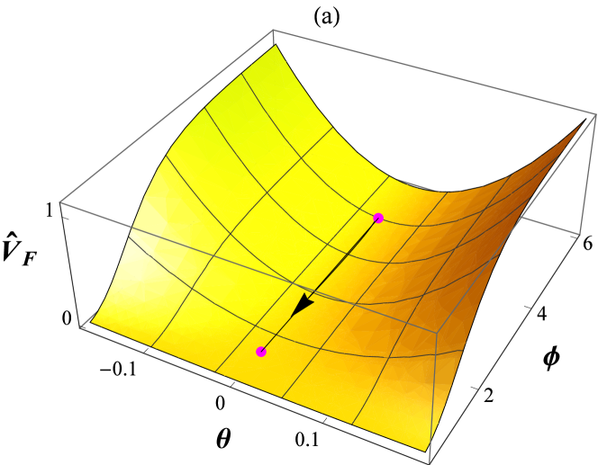
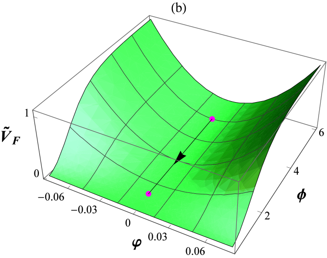
Figure 1: (a): Dependance of the potential on $\theta$ and $\phi$. $\hat{V}_{F}=V_{F}/(85\lambda_{e}^{2})$ and $\varphi\simeq 3\cdot 10^{-4}$ is taken. (b): Potential as a function of $\varphi$ and $\phi$. $\tilde{V}_{F}=V_{F}/(8\lambda_{e}^{2})$ and $\theta\simeq 0.012$ is taken. Both plots corresponds to the case (i) and $\omega=\pi+{\rm Arg}\left(\frac{V_{ud}}{V_{td}}\right)$ is taken. Arrows correspond to the inflaton’s path.

On the other hand, to guarantee the causality of fluctuations, the $N_{e}^{\rm inf}$ should satisfy Liddle:2003as :

$$N_{e}^{\rm inf}= 62-\ln\frac{k}{a_{0}H_{0}}-\ln\frac{10^{16}{\rm GeV}}{{\cal V}_{i}^{1/4}}+\ln\frac{{\cal V}_{i}^{1/4}}{{\cal V}_{e}^{1/4}}$$ (53)

$$-\frac{4-3\gamma}{3\gamma}\ln\frac{{\cal V}_{e}^{1/4}}{\rho_{reh}^{1/4}}~{},$$

where $k=0.002\hskip 1.70717pt{\rm Mpc}^{-1}$ and the present horizon scale $a_{0}H_{0}$ is $a_{0}H_{0}\approx 0.00033\hskip 1.70717pt{\rm Mpc}^{-1}$. The factor $\gamma=2\frac{\int_{0}^{\phi_{e}}(1-{\cal V}/{\cal V}_{e})^{1/2}d\phi}{\int_{0}^{\phi_{e}}(1-{\cal V}/{\cal V}_{e})^{-1/2}d\phi}$ (equals to$\simeq 1.19$ in our case) accounts for the effect of inflaton’s oscillation around its minima after inflation Turner:1983he . For consistency, we need to match the values of $N_{e}^{\rm inf}$ obtained from Eqs. (52) and (53). As it turns out, within the considered scenario $\phi_{i}\simeq 1.1295$ and $\phi_{e}\simeq 4.8325$ (given in the units of $M_{Pl}=2.4\times 10^{18}$ GeV). These points, together with the inflaton’s trajectory during the course of the inflations, are shown in plots of Fig.1. With $\phi_{i}$ get fixed, we can calculate the observables given in (50) and (51). These quantities are calculated by the parameters in (49). The latter are independent of the $\lambda_{e}$ -the single coupling appearing in (48). $\lambda_{e}$’s value is important for the value of the vacuum energy dominantly stored in the scalar potential ${\cal V}$ during the inflation. The values ${\cal V}_{i,e}$ are needed to carry calculations with Eq. (53). On the other hand, another observable - the amplitude of curvature perturbation $A_{s}$ given by

$$A_{s}^{1/2}=\frac{1}{\sqrt{12}\pi}\left|\frac{{\cal V}^{3/2}}{M_{Pl}^{3}{\cal V}^{\prime}}\right|_{\phi_{i}}~{},$$ (54)

can be used to determine ${\cal V}_{i}$ and consequently the value of $\lambda_{e}$. In order to get experimentally measured value $A_{s}^{1/2}=4.581\times 10^{-5}$ Akrami:2018odb , using (54), we need to have $\lambda_{e}(M_{Pl})=2.435\times 10^{-5}$ phi-val . This, in turn allows to determine the MSSM parameter $\tan\beta$ to be Yetanbt :

$$\tan\beta\simeq 13.12~{}.$$ (55)

In addition, calculation of the thermal energy density $\rho_{\rm reh}\!\!=\!\frac{\pi^{2}}{30}g_{*}T_{r}^{4}$ is required. It depends on the reheating process (via reheating temperature $T_{r}$) which is realized by the inflaton’s decay. In this case Kofman:1997yn :

$$T_{r}=\left(\frac{90}{\pi^{2}g_{*}}\right)^{1/4}\!\!\sqrt{M_{Pl}\Gamma(\phi)},$$ (56)

where $g_{*}$ is the effective number of massless degrees of freedon at temperature $T_{r}$ ($g_{*}\!=\!N_{b}\!+\!\frac{7}{8}N_{b}$ and in our case is $g_{*}\!\!=\!42.75$), and $\Gamma(\phi)$ is inflaton’s decay width. It turns out that within our model, all parameters involved in the inflation and in this process are known. This enables us to calculate $\Gamma(\phi)$ and therefore predict the $T_{r}$.

Since the inflaton comes from the MSSM states, its couplings to the remaining states are well fixed. The VEV configuration (33) breaks the $SU(3)_{c}\times SU(2)_{L}\times U(1)_{Y}$ symmetry down to the $SU(2)_{c}$. Thus, from the gauge sector only $SU(2)_{c}$’s states are massless. Via the Yukawa superpotential, the inflaton field couples to the MSSM chiral superfield states via the $z$ VEV. And the very same couplings generate masses (which scale as $z$ times corresponding Yukawa coupling) of the latter states. Because of this, it turns out that states which have tree level coupling with the inflaton are heavier than the inflaton. Therefore, inflaton’s tree level decays are either kinematically forbidden or (if realized via many body decays) are strongly suppressed.

The dominant decay of the inflaton $\phi$ happens radiatively (via 1-loop correction) in two massless gluons of the unbroken $SU(2)_{c}$. Corresponding decay width is given by:

$$\Gamma(\phi)\!\simeq\!\Gamma(\phi\to gg)\!=\!\frac{3m_{\phi}^{3}\alpha_{s}^{2}}{2(8\pi)^{3}}\left|\sum_{Q}f_{Q}A_{1/2}(\tau_{Q})\right|^{2}$$

$$\simeq\frac{m_{\phi}^{3}\alpha_{s}^{2}}{48\pi^{3}}\left(\frac{F^{\prime}}{F}+\frac{F_{g}^{\prime}}{F_{g}}\right)^{2}~{},$$ (57)

where $m_{\phi}^{2}={\cal V}^{\prime\prime}$ (is the inflaton’s mass), $\tau_{q}=\frac{m_{\phi}^{2}}{4m_{Q}^{2}}$ and $m_{Q}$ denote masses of $SU(2)_{c}$ colored fermions which couple with the inflaton. Among them are $SU(2)_{c}$ doublets from massive $s,b$ quarks, which circulate into the loop diagram. For them $f_{s,b}\!=\!\frac{F^{\prime}}{F}$ is taken in Eq. (III) . Their canonically normalized couplings to the inflaton emerges from the Yukawa term:

$$\frac{1}{2}F(\phi)d^{T}Y_{D}d^{c},~{} F(\phi)\!=\!\tanh\!\frac{\phi}{\sqrt{2}}(1\!-\!\tanh^{2}\!\!\frac{\phi}{\sqrt{2}})^{1/2},~{}$$ (58)

which for $\phi$-$d$-$d^{c}$-type interaction gives $\frac{1}{2}F^{\prime}\phi d^{T}Y_{D}d^{c}$, where $F^{\prime}=\frac{dF}{d\phi}$, and that’s how the term $\frac{F^{\prime}}{F}=f_{s,b}$ appears in Eq. (III). Besides these, in the loop (governing inflaton’s decay) two massive Dirac fermions circulate, which are formed after $SU(3)_{c}\to SU(2)_{c}$ breaking and pairing corresponding gauginos and colored matter. For them $f_{g}\!=\!\frac{F_{g}^{\prime}}{F_{g}}$ was used in (III) with $F_{g}(\phi)\!=\!\sinh\!\frac{\phi}{\sqrt{2}}$. The function $A_{1/2}(\tau_{Q})$ in Eq. (III) has property $\left.A_{1/2}(\tau_{Q})\right|_{\tau_{Q}\ll 1}\simeq 4/3$ Djouadi:2005gi . In (III) all $\phi$ dependent quantities need to be evaluated at point $\phi=\phi_{e}$.

Having all these expressions, we can carry out detailed analysis related to the inflation process. Doing so, for the observables we obtain phi-val :

$$n_{s}=0.9662,~{}~{}r=0.00118,~{}~{}\frac{dn_{s}}{d\ln k}=-5.98\cdot 10^{-4},$$

$$N_{e}^{\rm inf}=57.74,~{}~{}~{}\rho_{\rm reh}^{1/4}=2.61\cdot 10^{7}{\rm GeV},$$

$$T_{r}=1.35\cdot 10^{7}{\rm GeV}.$$ (59)

As one can see, the values of $n_{s},r$ and $\frac{dn_{s}}{d\ln k}$ are in good agreement with the current observations Akrami:2018odb . We will comment about the value of the reheating temperature $T_{r}$ in the next section, where some implications and related phenomenology are discussed.

IV IV. Related Phenomenology and Discussion

In this section, first we discuss some implications and phenomenology related to the inflationary scenario we have presented above and then give brief summary.

IV.1 IV.1. Relic gravitinos

For the reheat temperature $T_{r}$ obtained in this schenario [see Eq. (III)], the thermally produced gravitino abundance can easily be compatible TR-bounds with observations for specific and phenomenologically viable sparticle spectroscopy.

As far as the non-thermal gravitino production, via the inflaton decay is concerned, as shown in Nilles:2001fg , this process can be adequately suppressed. However, results of Nilles:2001fg applies for minimal Kähler potential. If nonminimal Kähler potential involves specific mixing terms between the inflaton $z$ (as denoted in the present work) and SUSY breaking superfield $X$, then situation in general would be different Dine:2006ii ; Endo:2006tf ; Kawasaki:2006hm . As was pointed out Dine:2006ii ; Kawasaki:2006hm , the additional $\delta{\cal K}=|z|^{2}X^{2}$ Kähler potential coupling, can lead to the gravitino overproduction. This term can be easily forbidden if $X$ field transforms either under some $U(1)$ or $R$-symmetry, or under discrete symmetry (such as for instance $Z_{3}$). Thus, the details of the SUSY breaking sector is important. On the other hand, connection of the SUSY breaking mechanism with our inflation model deserves separate investigation.

IV.2 IV.2. Neutrino masses

Within the considered scenario, in case (i) [see paragraph after Eq. (36)] the lepton number violating $W^{\prime}=-\lambda q_{1}l_{2}d^{c}$ superpotential coupling, which also breaks matter parity, was exploited. This, at 1-loop level induce $\mu_{i}h_{u}l_{i}$-type superpotential and soft $B_{i}h_{u}\tilde{l}_{i}$ terms, which result neutrino mass $m_{\nu_{\mu}}\!\approx\!\frac{\lambda^{2}g_{2}^{2}}{4c_{w}^{2}}\frac{m_{d}^{2}}{\tilde{m}}\!\left(\!\frac{9}{8\pi^{2}}\ln\frac{M_{Pl}}{M_{Z}}\!\right)^{2}$ Rpar , by neutralino exchange [similar to seesaw induced neutrino mass, generated by the right handed neutrino (RHN) exchange], where $\tilde{m}$ is the SUSY scale (for simplicity we have assumed that all sparticles have masses close to $\tilde{m}$). This, by demanding $m_{\nu}\stackrel{{\scriptstyle<}}{{\sim}}0.1$ eV for $\tilde{m}=2$ TeV gives the bound $\lambda\stackrel{{\scriptstyle<}}{{\sim}}0.1$. This, together with desirably suppressed value of $\tan\theta\simeq\frac{\lambda_{d}}{\lambda}<0.1$ gives $6\times 10^{-4}\stackrel{{\scriptstyle<}}{{\sim}}\lambda\stackrel{{\scriptstyle<}}{{\sim}}0.1$. The $\lambda q_{1}l_{2}d^{c}$ superpotential coupling term also directly contribute to the 1-loop neutrino mass$\sim\frac{3\lambda^{2}}{8\pi^{2}}\frac{m_{d}^{2}}{\tilde{m}}$ Rpar . This, for $\lambda\stackrel{{\scriptstyle<}}{{\sim}}0.1$ gives more suppressed contribution $\delta m_{\nu}\stackrel{{\scriptstyle<}}{{\sim}}2\times 10^{-3}$ eV. Although these neutrino mass scales are close to the values needed for accommodation of the neutrino data nu-data , by the $W^{\prime}=-\lambda q_{1}l_{2}d^{c}$ coupling alone would be hard and challenging to get also desirable neutrino mixing pattern. To achieve all these, one way is to include additional $\bar{\lambda}_{ijk}e^{c}_{i}l_{j}l_{k}$ and $\lambda_{ijk}q_{i}l_{j}d^{c}_{k}$-type terms, and by proper selection of various couplings obtain consistent neutrino sector. However, within our study, one should also take care that considered inflation model remains intact. Alternative, and perhaps simpler, way would be to include RHN state(s), which can lead to desirable neutrino oscillations via the contribution of conventional seesaw mechanism see-saw . This possibility definitely seems the simplest choice especially for our case (ii), which preserves matter parity and lepton number. Detailed study of the neutrino sector in connection to the considered model of inflation should be pursued elsewhere.

Concluding, within the MSSM we have presented model of inflation in which the inflaton is a combination of the Higgs, slepton and squark states. While the VEVs of these states are along the flat $D$-term trajectory, the inflation is driven by the vacuum energy of the electron Yukawa superpotential. This uniquely fixes the value of the MSSM parameter $\tan\beta$ [see Eq. (55)]. To our knowledge, it is first example with such close connection between the particle physics model and inflationary cosmology. Since all parameters involved in the inflation and postinflationary reheating processes were known, the presented model is very predictive.

Encouraged by these findings, would be interesting to realise similar constructions in a framework of other well motivated SUSY constructions such as left-right symmetric and grand unified [i.e. $SU(5)$, $SO(10)$, etc.] models. Note that, if within the GUTs, inflaton condensate (being either Higgs, slepton or squark state) breaks the GUT symmetry, then (as shown in Ref. Dvali:1998ct ) within such construction the monopole problem can be easily avoided. Investigation of these exciting issues will be performed elsewhere.

References

- (1) Y. Akrami et al. [Planck Collaboration], arXiv:1807.06211 [astro-ph.CO].
- (2) A. H. Guth, Phys. Rev. D 23 (1981) 347; A. D. Linde, Phys. Lett. B 108, 389 (1982).
- (3) E. J. Copeland, A. R. Liddle, D. H. Lyth, E. D. Stewart and D. Wands, Phys. Rev. D 49, 6410 (1994); G. R. Dvali, Q. Shafi and R. K. Schaefer, Phys. Rev. Lett. 73, 1886 (1994).
- (4) M. B. Einhorn and D. R. T. Jones, JHEP 1003, 026 (2010); S. Ferrara, R. Kallosh, A. Linde, A. Marrani and A. Van Proeyen, Phys. Rev. D 82, 045003 (2010); H. M. Lee, JCAP 1008, 003 (2010); For a review and references see: T. Terada, arXiv:1508.05335 [hep-th].
- (5) R. Allahverdi, K. Enqvist, J. Garcia-Bellido and A. Mazumdar, Phys. Rev. Lett. 97, 191304 (2006); R. Allahverdi, B. Dutta and A. Mazumdar, Phys. Rev. D 75, 075018 (2007); For a review and references see: J. Martin, C. Ringeval and V. Vennin, Phys. Dark Univ. 5-6, 75 (2014).
- (6) See Ref. in susy-infl and also: G. R. Dvali, L. M. Krauss and H. Liu, hep-ph/9707456; G. R. Dvali, G. Lazarides and Q. Shafi, Phys. Lett. B 424, 259 (1998); R. Jeannerot, S. Khalil, G. Lazarides and Q. Shafi, JHEP 0010, 012 (2000); G. Lazarides, Lect. Notes Phys. 592, 351 (2002) [hep-ph/0111328]. S. Antusch, M. Bastero-Gil, S. F. King and Q. Shafi, Phys. Rev. D 71, 083519 (2005); J. Ellis, H. J. He and Z. Z. Xianyu, Phys. Rev. D 91, no. 2, 021302 (2015); B. C. Bryant and S. Raby, Phys. Rev. D 93, no. 9, 095003 (2016); M. A. Masoud, M. U. Rehman and M. M. A. Abid, International Journal of Modern Physics D (Oct 2019), [arXiv:1910.10519 [hep-ph]];
- (7) Z. Tavartkiladze, Phys. Rev. D 100, no. 9, 095027 (2019).
- (8) S. Ferrara, M. Kaku, P. K. Townsend and P. van Nieuwenhuizen, Nucl. Phys. B 129, 125 (1977); M. Kaku, P. K. Townsend and P. van Nieuwenhuizen, Phys. Rev. D 17, 3179 (1978); E. Cremmer, B. Julia, J. Scherk, S. Ferrara, L. Girardello and P. van Nieuwenhuizen, Nucl. Phys. B 147, 105 (1979);
-
(9)
T. Kugo and S. Uehara,
“Improved Superconformal Gauge Conditions in the Supergravity Yang-Mills Matter System,”
Nucl. Phys. B 222, 125 (1983);
V. Kaplunovsky and J. Louis, “Field dependent gauge couplings in locally supersymmetric effective quantum field theories,” Nucl. Phys. B 422, 57 (1994). - (10) R. Kallosh and A. Linde, JCAP 1307, 002 (2013); R. Kallosh, A. Linde and D. Roest, JHEP 1311, 198 (2013).
- (11) S. Ferrara and R. Kallosh, Phys. Rev. D 94, no. 12, 126015 (2016); R. Kallosh, A. Linde, T. Wrase and Y. Yamada, JHEP 1704, 144 (2017).
- (12) I. Affleck and M. Dine, Nucl. Phys. B 249, 361 (1985).
- (13) M. Dine, L. Randall and S. D. Thomas, Nucl. Phys. B 458, 291 (1996).
- (14) E. Cremmer, S. Ferrara, L. Girardello and A. Van Proeyen, Phys. Lett. 116B, 231 (1982); J. A. Bagger, Nucl. Phys. B 211, 302 (1983); E. Cremmer, S. Ferrara, L. Girardello and A. Van Proeyen, Nucl. Phys. B 212, 413 (1983); For detailed discussions see the textbook: J. Wess and J. Bagger, “Supersymmetry and supergravity”.
- (15) T. Gherghetta, C. F. Kolda and S. P. Martin, Nucl. Phys. B 468, 37 (1996).
- (16) Since within the considered scenario the inflation occurs at high scales (with large values of the inflaton), upon the calculations we use the RG evaluated values of the Yukawa couplings, masses and the CKM matrix elements at scale .
- (17) Strictly speaking, the value of should be found from the minimization of the whole potential. However, since for both cases we consider , with improved accuracy we will have and for cases (i) and (ii) respectively. For and additional corrections are and we do not need to include them in our considerations because in practice they are insignificunt.
- (18) Near the SUSY scale, between the and we have the relation: .
- (19) E. D. Stewart and D. H. Lyth, Phys. Lett. B 302, 171 (1993).
- (20) A. R. Liddle, P. Parsons and J. D. Barrow, Phys. Rev. D 50, 7222 (1994).
- (21) J. E. Lidsey, A. R. Liddle, E. W. Kolb, E. J. Copeland, T. Barreiro and M. Abney, Rev. Mod. Phys. 69, 373 (1997); A. R. Liddle and S. M. Leach, Phys. Rev. D 68, 103503 (2003).
- (22) M. S. Turner, Phys. Rev. D 28, 1243 (1983).
- (23) L. Kofman, A. D. Linde and A. A. Starobinsky, Phys. Rev. D 56, 3258 (1997).
- (24) For expressions see for instance: A. Djouadi, Phys. Rept. 457, 1 (2008); and references therein.
- (25) M. Kawasaki, K. Kohri and T. Moroi, Phys. Rev. D 71, 083502 (2005); M. Kawasaki, K. Kohri, T. Moroi and Y. Takaesu, Phys. Rev. D 97, no. 2, 023502 (2018).
- (26) H. P. Nilles, M. Peloso and L. Sorbo, JHEP 0104, 004 (2001).
- (27) M. Dine, R. Kitano, A. Morisse and Y. Shirman, Phys. Rev. D 73, 123518 (2006).
- (28) M. Endo, K. Hamaguchi and F. Takahashi, Phys. Rev. D 74, 023531 (2006).
- (29) M. Kawasaki, F. Takahashi and T. T. Yanagida, Phys. Rev. D 74, 043519 (2006).
- (30) T. Banks, Y. Grossman, E. Nardi and Y. Nir, Phys. Rev. D 52, 5319 (1995); R. Hempfling, Nucl. Phys. B 478, 3 (1996); H. P. Nilles and N. Polonsky, Nucl. Phys. B 484, 33 (1997); E. Nardi, Phys. Rev. D 55, 5772 (1997).
- (31) I. Esteban, M. C. Gonzalez-Garcia, M. Maltoni, I. Martinez-Soler and T. Schwetz, JHEP 1701, 087 (2017); F. Capozzi, E. Di Valentino, E. Lisi, A. Marrone, A. Melchiorri and A. Palazzo, Phys. Rev. D 95, no. 9, 096014 (2017).
- (32) P. Minkowski, Phys. Lett. 67B, 421 (1977); M. Gell-Mann, P. Ramond, and R. Slansky, Conf. Proc. C 790927, 315 (1979); T. Yanagida, Conf. Proc. C 7902131, 95 (1979); R. N. Mohapatra and G. Senjanovic, Phys. Rev. Lett. 44, 912 (1980).
- (33) G. R. Dvali and L. M. Krauss, hep-ph/9811298.