Stable multi-peak vector solitons in spin-orbit coupled spin-$1$ polar condensates

Abstract

We demonstrate the formation of multi-peak three-component stationary stripe vector solitons in a quasi-one-dimensional spin-orbit-coupled hyper-fine spin $F=1$ polar Bose-Einstein condensate. The present investigation is carried out through a numerical solution by imaginary-time propagation and an analytic variational approximation of the underlying mean-field Gross-Pitaevskii equation. Simple analytic results for energy and component densities were found to be in excellent agreement with the numerical results for solitons with more than 100 pronounced maxima and minima. The vector solitons are one of the two types: dark-bright-dark or bright-dark-bright. In the former a maximum density in component $F_{z}=0$ at the center is accompanied by a zero in components $F_{z}=\pm 1$. The opposite happens in the latter case. The vector solitons are demonstrated to be mobile and dynamically stable. The collision between two such vector solitons is found to be quasi elastic at large velocities with the conservation of total density of each vector soliton. However, at very small velocity, the collision is inelastic with a destruction of the initial vector solitons. It is possible to observe and study the predicted SO-coupled vector solitons in a laboratory.

1 Introduction

A soliton or solitary wave is a self-reinforcing wave packet that maintains its shape while propagating at a constant velocity. Solitons are created by a cancellation of nonlinear and dispersive effects in the medium. Solitons have been observed [1] in water waves, in non-linear optics, and in Bose-Einstein condensates (BECs) among others. Solitons have been generated in a BEC of ⁷Li [2] and ⁸⁵Rb [3] atoms by manipulating the non-linear atomic attraction near a Feshbach resonance [4]. Solitons have also been studied in binary BEC mixtures [5]. Properties of BEC solitons are well described [6] by the mean-field Gross-Pitaevskii (GP) equation [7].

The experimental realization of a spinor BEC of ²³Na atoms with hyper-fine spin $F=1$ [8] required a generalization of the GP equation [9], which can describe its properties. In a spinor BEC of neutral atoms, there is no natural spin-orbit (SO) coupling. However, a synthetic SO coupling can realized in a spinor BEC by a management of external electromagnetic fields [10, 11]. Different managements are possible which generate different types of SO coupling between spin and momentum in a spinor BEC. Two such possible SO couplings are due to Rashba [12] and Dresselhaus [13]. An equal-strength mixture of Rashba and Dresselhaus SO couplings was first realized experimentally in a pseudo spin-1/2 spinor BEC formed of two ($F_{z}=0$ and $-1$) of the three hyper-fine spin components of the $F=1$ state 5S_1/2 of ⁸⁷Rb [14]. The coupling scheme of this truncated two-component spinor BEC is quite similar to that of a spin-1/2 particle and can be described by the Pauli spin-1/2 spinors. This is why this dynamics is ususlly termed pseudo-spin-1/2 dynamics. Similar SO-coupled BECs were formed later and studied in different laboratories [15]. Different possible SO couplings in spinor BECs and the ways to engineer these in a laboratory are addressed in review articles [10]. Possible ways of realizing the SO coupling in three-component spin-1 BEC have been discussed [16].

Solitons have been extensively studied in spinor BECs without SO coupling [17]. Solitonic structures in SO-coupled pseudo-spin-$1/2$ [18, 19], spin-$1$ [20, 21] and spin-2 [22] BECs have also been investigated theoretically. These studies were extended to quasi-solitons confined in two [23] and three [24] dimensions. Different types of SO coupling introduce rich dynamics through different types of derivative couplings among the component wave functions of the mean-field model.

A spin-$1$ spinor BEC is controlled by two interaction strengths, e.g., $c_{0}\propto(a_{0}+2a_{2})/3$ and $c_{2}\propto(a_{2}-a_{0})/3$, with $a_{0}$ and $a_{2}$ the scattering lengths in total spin $0$ and 2 channels, respectively [9]. All spin-1 spinor BECs can be classified into two distinct types [9, 10]: a ferromagnetic BEC ($c_{2}<0$) and an anti-ferromagnetic or a polar BEC ($c_{2}>0$). Most of the previous studies on SO-coupled BEC soliton [18] were limited to the pseudo-spin-1/2 case, which does and can not exhibit the full rich dynamics of a spin-1 spinor. Like its three-component counterpart, a pseudo-spin-1/2 spinor does not have the distinct varieties: ferromagnetic and polar. For example, an SO-coupled spin-1 polar soliton is a stripe multi-peak one, whereas the ferromagnetic soliton is a single-peak one [21].

In this paper, we study vector solitons in a SO-coupled spin-$1$ polar BEC using a mean-field coupled GP equation. We consider the SO coupling $(\propto\gamma p_{x}\Sigma_{y})$, which is an equal-strength mixture of Rashba and Dresselhaus SO couplings realized in the pioneering experiment [14]. Here $p_{x}$ is the $x$ component of momentum, $\gamma$ the strength of SO coupling, and $\Sigma_{y}$ is the $y$ component of the spin-1 matrix $\Sigma$. With this SO coupling, we study the properties of three-component vector solitons in a one-dimensional (1D) polar BEC along the $x$ axis [21]. The polar solitons generated with the SO coupling $(\propto\gamma p_{x}\Sigma_{y})$ have identical density distribution and energy as the solitons with the SO coupling $(\propto\gamma p_{x}\Sigma_{x})$. Because of the rotational symmetry in spin space around the symmetry axis $z$, these two SO couplings are equivalent. The generated vector solitons can have a very large number of pronounced maxima and minima along the spatial direction and hence are stripe vector solitons [19]. We demonstrate the formation of stable robust stationary vector solitons, with more than 100 maxima and minima, numerically by imaginary-time propagation.

Simple analytic expression for the densities and energies of the vector soliton were obtained from the SO-coupled GP equation employing a plausible approximation and a variational scheme which minimize the energy functional. It is remarkable that the analytic results are independent of the interaction strength $c_{2}$ determined only by the strength $c_{0}$. The analytic results for the density and energy of the SO-coupled polar vector soliton are found to be in excellent agreement with the numerical results of the same obtained by imaginary-time propagation. The numerical results, however, has a weak dependence on the interaction strength $c_{2}$.

We also study the dynamics of the vector soliton numerically by real-time simulation. The dynamical stability of the vector soliton was established. The collision between two solitons is found to be quasi elastic at large velocities with the conservation of total density of each vector soliton. The component densities are not conserved as the SO-coupled GP equation is not Galilean invariant [21]. The collision dynamics at small velocity of two vector solitons is found to be inelastic with the destruction of the individual solitons.

In Sec. 2, we describe the mean-field model GP equation for a SO-coupled spin-$1$ polar BEC and provide an analytic variational solution of this model using a Gaussian and a hyperbolic secant form of the wave-function profile to study the SO-coupled spin-1 polar soliton. In Sec. 3, we provide a numerical solution of the model by imaginary-time propagation and compare the results for density and energy with the corresponding analytic variational results. We also study the dynamics of the vector soliton by real-time propagation. The solitons were demonstrated to be dynamically stable. The collision dynamics of two vector solitons was also studied at different colliding velocities. In Sec. 4 a summary of our findings is presented.

2 Mean-field model for a SO-coupled BEC

We consider a SO-coupled spinor BEC confined in 1D along the $x$ axis. The 1D confinement is realized by strong traps in $y$ and $z$ directions, so that the essential dynamics of the system takes place along the $x$ axis [25], while in the transverse $y$ and $z$ directions the system is frozen in Gaussian ground states. The single particle Hamiltonian of the condensate in this quasi-1D trap is taken in scaled dimensionless units $\hbar={\bar{\bf m}}=1$ as [26]

$$H_{0}=\frac{p_{x}^{2}}{2}+\gamma p_{x}\Sigma_{y},$$ (1)

where $\bar{\bf m}$ is the mass of an atom, $p_{x}=-i\partial/\partial x$ is the momentum operator along $x$ axis, and $\Sigma_{y}$ is the irreducible representation of the $y$ component of the spin-1 matrix:

$$\Sigma_{y}=\frac{i}{\sqrt{2}}\left(\begin{array}[]{ccccc}0&-1&0\\ 1&0&-1\\ 0&1&0\end{array}\right).$$ (5)

As we will be investigating vector solitons, we will not include any trapping potential in the Hamiltonian.

Using the single particle model Hamiltonian (1) and considering interactions in the Hartree approximation, the 1D [25] spin-1 BEC of $N$ atoms can be described by the following set of three coupled mean-field partial differential time-dependent GP equations for the wave-function components $\phi_{j}$ [9]

$$i\frac{\partial\phi_{\pm 1}}{\partial{t}} =\left(-\frac{1}{2}\frac{\partial^{2}}{\partial{x}^{2}}+{c}_{0}{\rho}\right)\phi_{\pm 1}{\mp}\frac{{\gamma}}{\sqrt{2}}\frac{\partial\phi_{0}}{\partial x}$$

$$+c_{2}({\rho}_{\pm 1}+{\rho}_{0}-{\rho}_{\mp 1})\phi_{\pm 1}+c_{2}\phi_{0}^{2}\phi_{\mp 1}^{*},$$ (6)

$$i\frac{\partial\phi_{0}}{\partial{t}} =\left(-\frac{1}{2}\frac{\partial^{2}}{\partial{x}^{2}}+{c}_{0}{\rho}\right)\phi_{0}{+}\frac{{\gamma}}{\sqrt{2}}\left[\frac{\partial\phi_{+1}}{\partial x}{-}\frac{\partial\phi_{-1}}{\partial x}\right]$$

$$+c_{2}({\rho}_{+1}+{\rho}_{-1})\phi_{0}+2{c}_{2}\phi_{0}^{*}\phi_{+1}\phi_{-1},$$ (7)

where we have suppressed the space and time dependence of the wave function $\phi_{\pm 1,0}(x,t)$, $c_{0}$ and $c_{2}$ are the interaction strengths, ${\rho}_{j}=|\phi_{j}|^{2}$ where $j=+1,0,-1$ are the component densities corresponding to the three spin components, and ${\rho}=(\rho_{+1}+\rho_{0}+\rho_{-1})$ is the conserved total density normalized to unity, i.e., $\int_{-\infty}^{\infty}{\rho}({x})d{x}=1.$ The conserved magnetization is defined as $\int_{-\infty}^{\infty}dx(\rho_{+1}-\rho_{-1})=m.$

The energy functional corresponding to the mean-field SO-coupled spinor BEC model (6) and (7) is [27]

$$E(\gamma) \equiv E_{1}(\gamma)+E_{2}(\gamma)$$

$$=\int_{-\infty}^{\infty}dx\bigg{[}\frac{1}{2}\left|\frac{d\phi_{+1}}{dx}\right|^{2}+\frac{1}{2}\left|\frac{d\phi_{0}}{dx}\right|^{2}+\frac{1}{2}\left|\frac{d\phi_{-1}}{dx}\right|^{2}$$

$$+\frac{c_{0}}{2}\rho^{2}+\frac{c_{2}}{2}\Big{\{}\rho_{+1}^{2}+\rho_{-1}^{2}+2\big{(}\rho_{+1}\rho_{0}-\rho_{-1}\rho_{+1}$$

$$+\rho_{-1}\rho_{0}+\phi_{-1}^{*}\phi_{0}^{2}\phi_{+1}^{*}+\phi_{-1}\phi_{0}^{*2}\phi_{+1}\big{)}\Big{\}}\bigg{]}$$

$$+\int_{-\infty}^{\infty}dx\bigg{[}\frac{\gamma}{\sqrt{2}}\Big{\{}\phi_{0}^{*}\Big{(}\frac{d\phi_{+1}}{dx}-\frac{d\phi_{-1}}{dx}\Big{)}$$

$$-\left(\phi_{+1}^{*}-\phi_{-1}^{*}\right)\frac{d\phi_{0}}{dx}\Big{\}}\bigg{]}.$$ (8)

For magnetization $m=0$, it is possible to develop a variational approximation for the stationary problem valid for a polar BEC ($c_{2}>0$). For $m=0$, we minimize this energy functional using an analytic variational wave function to find the analytic solution of the SO-coupled GP equation.

A stationary vector soliton is described by the time-independent version of GP equations (6) and (7) obtained by replacing the terms $i\partial\phi_{j}/dt$ by $\mu_{j}\phi_{j}$, where $\mu_{j}$s are the chemical potentials. An analytic approximation scheme for the solution of these time-independent equations for a stationary vector soliton is constructed by approximating these solutions in terms of a linear combination of analytic solutions of the linear version of these equations obtained by setting $c_{0}=0$, and $c_{2}=0$:

$${E\phi_{\pm 1}} =-\frac{1}{2}\frac{\partial^{2}\phi_{\pm 1}}{\partial{x}^{2}}{\mp}\frac{{\gamma}}{\sqrt{2}}\frac{\partial\phi_{0}}{\partial x},$$ (9)

$${E\phi_{0}} =-\frac{1}{2}\frac{\partial^{2}\phi_{0}}{\partial{x}^{2}}{+}\frac{{\gamma}}{\sqrt{2}}\left[\frac{\partial\phi_{+1}}{\partial x}{-}\frac{\partial\phi_{-1}}{\partial x}\right],$$ (10)

with $E$ the energy. Equations (9) and (10) have the following degenerate solutions

$$\widetilde{\Phi}_{1}(x)\equiv\left(\begin{array}[]{c}\widetilde{\phi}_{+1}\\ \widetilde{\phi}_{0}\\ \widetilde{\phi}_{-1}\end{array}\right)=\frac{e^{i\gamma x}}{2}\left(\begin{array}[]{c}1\\ -i\sqrt{2}\\ -1\end{array}\right),$$ (17)

$$\widetilde{\Phi}_{2}(x)\equiv\left(\begin{array}[]{c}\widetilde{\phi}_{+1}\\ \widetilde{\phi}_{0}\\ \widetilde{\phi}_{-1}\end{array}\right)=\frac{e^{-i\gamma x}}{2}\left(\begin{array}[]{c}1\\ i\sqrt{2}\\ -1\end{array}\right),$$ (24)

each of energy $E=-\gamma^{2}/2$.

The analytic ansatz for the stationary wave functions of Eqs. (6) and (7) are taken as the following linear combination of solutions (17) and (24):

$$\Phi_{1}(x)\equiv\left(\begin{array}[]{c}\phi_{+1}\\ \phi_{0}\\ \phi_{-1}\end{array}\right)= \frac{\psi(x)}{\sqrt{2}}\left[\widetilde{\Phi}_{1}(x)+\widetilde{\Phi}_{2}(x)\right]$$ (28)

$$= \frac{\psi(x)}{\sqrt{2}}\left(\begin{array}[]{c}\cos(\gamma x)\\ \sqrt{2}\sin(\gamma x)\\ -\cos(\gamma x)\end{array}\right),$$ (32)

$$\Phi_{2}(x)\equiv\left(\begin{array}[]{c}\phi_{+1}\\ \phi_{0}\\ \phi_{-1}\end{array}\right)= \frac{\psi(x)}{\sqrt{2}}\left[\widetilde{\Phi}_{1}(x)-\widetilde{\Phi}_{2}(x)\right]$$ (36)

$$= \frac{i\psi(x)}{\sqrt{2}}\left(\begin{array}[]{c}\sin(\gamma x)\\ -\sqrt{2}\cos(\gamma x)\\ -\sin(\gamma x)\end{array}\right),\quad$$ (40)

where $\psi(x)$ is a normalized localized function. The forms (32) and (40) are also motivated by a prior study of numerical results, which reveals that the component densities have the same localized shape [28], but with different normalizations, modulated sinusoidally with a spatial frequency of $\gamma/\pi$ and that a maximum density of components $j=\pm 1$ is accompanied by a minimum density of component $j=0$ and vice versa. The spatial density modulation frequency $\gamma/\pi$ appears naturally by construction through the sine and cosine terms.

We will consider the following Gaussian and secant hyperbolic ansatz for the function $\psi(x)$ in Eqs. (32)-(40)

$$\psi(x) ={\frac{1}{\sqrt{\alpha\sqrt{\pi}}}}\exp\left[-\frac{x^{2}}{2\alpha^{2}}\right],$$ (41)

$$\psi(x) =\frac{\sqrt{\sigma}}{\sqrt{2}}{\mathrm{sech}}(\sigma x).$$ (42)

With these ansatz for the wave function, the energy functional (2) is explicitly real, has the correct $\gamma$ dependence, magnetization ($m=0$) and normalization ($=1$). Ansatz (32) for the wave function has maxima of density at center ($x=0$) in components $j=\pm 1$ given by cosine functions and a minimum (zero) in density at center in component $j=0$ and is a vector soliton of type bright-dark-bright. Ansatz (40), on the other hand, corresponds to a maximum of density at center in component $j=0$ accompanied by minima (zero) of density at center in components $j=\pm 1$ and is a vector soliton of type dark-bright-dark. The numerical solution has exactly the same behavior. As confirmed by our numerical solution and analytic approximation, these two types of vector solitons have the same energy and are degenerate states.

With the analytic ansatz (32), and also (40), for the profile of the vector soliton, the energy functional (2) with function (41) can be evaluated to yield

$$E(\gamma)=-\frac{\gamma^{2}}{2}+\frac{1}{4\alpha^{2}}+\frac{c_{0}}{2\alpha\sqrt{2\pi}}.$$ (43)

The width $\alpha$ of the minimum-energy ground state vector soliton is obtained by minimizing this energy functional with respect to $\alpha$:

$$\alpha=-\frac{\sqrt{2\pi}}{c_{0}}.$$ (44)

For this width to be positive we require $c_{0}<0$. This width is independent of the SO-coupling strength $\gamma$ and interaction strength $c_{2}$. The following minimum of energy as a function of $\gamma$ is obtained by substituting Eq. (44) in Eq. (43)

$$E(\gamma)=-\frac{\gamma^{2}}{2}-\frac{c_{0}^{2}}{8\pi},$$ (45)

which is the energy of the minimum-energy spin-1 three-component vector soliton in the ground state. The corresponding expression for the function (41) is

$$\psi(x)=\left(\frac{c_{0}^{2}}{2\pi^{2}}\right)^{1/4}\exp\left(-\frac{c_{0}^{2}x^{2}}{4\pi}\right).$$ (46)

We note that the analytic variational results (45) and (46) for the energy and the wave function, respectively, are determined by the interaction parameter $c_{0}$ only and independent of the interaction strength $c_{2}$.

With both ansatz (32) and (40), employing the secant hyperbolic function (42), the energy functional becomes [21]

$$E(\gamma)=-\frac{\gamma^{2}}{2}+\frac{\sigma^{2}+c_{0}\sigma}{6},$$ (47)

which is minimized at

$$\sigma=-\frac{c_{0}}{2}$$ (48)

yielding the energy minimum

$$E(\gamma)=-\frac{\gamma^{2}}{2}-\frac{c_{0}^{2}}{24}$$ (49)

and the function (42)

$$\psi(x)=\frac{\sqrt{|c_{0}|}}{2}\mathrm{sech}\left(\frac{|c_{0}|x}{2}\right).$$ (50)

We find that the analytic energy (49) is smaller than energy (45). Due to the variational nature of the analytic calculation, energy (49) is closer to the exact energy and hence the secant hyperbolic form (50) of the wave function is a better approximation to the exact solution than the Gaussian form (46).

In one dimension, for a spin-1 spinor BEC, there are two other linearly independent SO couplings: $\gamma p_{x}\Sigma_{x}$ [21] and $\gamma p_{x}\Sigma_{z}$ [26], where

$$\Sigma_{x}=\frac{1}{\sqrt{2}}\left(\begin{array}[]{ccccc}0&1&0\\ 1&0&1\\ 0&1&0\end{array}\right),\quad\Sigma_{z}=\left(\begin{array}[]{ccccc}1&0&0\\ 0&0&0\\ 0&0&1\end{array}\right),$$ (57)

Of these, the SO coupling $\gamma p_{x}\Sigma_{x}$, like the SO coupling $\gamma p_{x}\Sigma_{y}$, connects the components $F_{z}=\pm 1$ with the component $F_{z}=0$ and these two SO couplings are equivalent and have identical analytic variational solution. To demonstrate this claim explicitly, we note that for SO coupling $\gamma p_{x}\Sigma_{x}$ the mean-field GP equation is [29]

$$i\frac{\partial\phi_{\pm 1}}{\partial{t}} =\left(-\frac{1}{2}\frac{\partial^{2}}{\partial{x}^{2}}+{c}_{0}{\rho}\right)\phi_{\pm 1}{\color[rgb]{1,0,0}-}\frac{{i\gamma}}{\sqrt{2}}\frac{\partial\phi_{0}}{\partial x}$$

$$+c_{2}({\rho}_{\pm 1}+{\rho}_{0}-{\rho}_{\mp 1})\phi_{\pm 1}+c_{2}\phi_{0}^{2}\phi_{\mp 1}^{*},$$ (58)

$$i\frac{\partial\phi_{0}}{\partial{t}} =\left(-\frac{1}{2}\frac{\partial^{2}}{\partial{x}^{2}}+{c}_{0}{\rho}\right)\phi_{0}{\color[rgb]{1,0,0}-}\frac{{i\gamma}}{\sqrt{2}}\left[\frac{\partial\phi_{+1}}{\partial x}{\color[rgb]{1,0,0}+}\frac{\partial\phi_{-1}}{\partial x}\right]$$

$$+c_{2}({\rho}_{+1}+{\rho}_{-1})\phi_{0}+2{c}_{2}\phi_{0}^{*}\phi_{+1}\phi_{-1}.$$ (59)

The energy functional is again given by (2) but now with $E_{2}(\gamma)$ given by

$$E_{2}(\gamma) =\int_{-\infty}^{\infty}dx\bigg{[}-\frac{i\gamma}{\sqrt{2}}\Big{\{}\phi_{0}^{*}\Big{(}\frac{d\phi_{+1}}{dx}+\frac{d\phi_{-1}}{dx}\Big{)}$$

$$+\left(\phi_{+1}^{*}+\phi_{-1}^{*}\right)\frac{d\phi_{0}}{dx}\Big{\}}\bigg{]}.$$ (60)

The analytic ansatz for the wave function in this case can be one of the following forms

$$\Phi_{1}\equiv \left(\begin{array}[]{c}\phi_{+1}\\ \phi_{0}\\ \phi_{-1}\end{array}\right)=\frac{\psi(x)}{\sqrt{2}}\left(\begin{array}[]{c}\cos(\gamma x)\\ -i\sqrt{2}\sin(\gamma x)\\ \cos(\gamma x)\end{array}\right),\quad$$ (67)

$$\Phi_{2}\equiv \left(\begin{array}[]{c}\phi_{+1}\\ \phi_{0}\\ \phi_{-1}\end{array}\right)=\frac{\psi(x)}{\sqrt{2}}\left(\begin{array}[]{c}\sin(\gamma x)\\ i\sqrt{2}\cos(\gamma x)\\ \sin(\gamma x)\end{array}\right).$$ (74)

With these forms the energy functional are explicitly real. Although the wave functions (67) and (74) on one hand, and (32) and (40) on the other hand are different, they lead to the same densities $\rho_{j}(x)$ and energies $E(\gamma)$. With the forms (67) and (74), the expression for the energy functional for a BEC with SO coupling $\gamma p_{x}\Sigma_{x}$ becomes identical with the expression for the energy functional for a BEC with SO coupling $\gamma p_{x}\Sigma_{y}$ for both Gaussian and secant hyperbolic ansatz (41) and (42) for the function $\psi(x)$. Hence the analytic solutions for the function $\psi(x)$ for SO coupling $\gamma p_{x}\Sigma_{x}$ are also given by (46) and (50), respectively, for the Gaussian and secant hyperbolic functions. However, the SO coupling $\gamma p_{x}\Sigma_{z}$ has a distinct coupling scheme and will be considered elsewhere.

3 Result and Discussion

We numerically solve the coupled partial differential equations (6)-(7) using the split-time-step Crank-Nicolson method [30] by real- and imaginary-time propagation methods. For a numerical simulation there are the Fortran [30] and C [31] programs and their open-multiprocessing [32] versions appropriate for using in multi-core processors. The ground state is determined by solving (6)-(7) using imaginary time propagation, which neither conserves normalization nor magnetization. Both normalization and magnetization can be fixed by renormalizing the wave-function components appropriately after each time iteration [27]. The initial wave function in imaginary-time propagation is taken as the variational function (32) or (40) with the Gaussian or secant hyperbolic form for the function $\psi(x)$ given by (46) or (50), respectively. The choice (32) leads to a vector soliton of type bright-dark-bright and the choice (32) generating the degenerate one of type dark-bright-dark. If we just take a localized function as the initial state without sine or cosine modulation the final state will be one of these two degenerate solutions. The real-time propagation method was used to study the dynamics with the converged solution obtained in imaginary-time propagation as the initial state. The space and time steps employed in the imaginary-time propagation are $dx=0.025$ and $dt=0.0001$ and that in the real-time propagation are $dx=0.025$ and $dt=0.00001$.

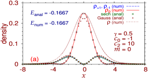
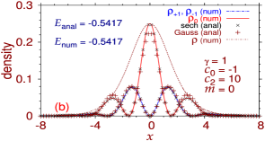
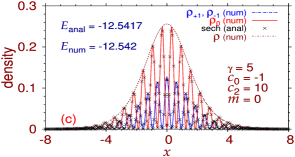
Figure 1: (Color online) Numerical (num) and analytic variational (anal) densities with the secant hyperbolic (sech) and Gaussian (Gauss) functions $\rho_{j}(x)\equiv|\phi_{j}|^{2},j=0,\pm 1$ of the three components for the lowest-energy vector soliton with $c_{0}=-1$, $c_{2}=10,m=0$, for (a) $\gamma=0.5,$ (b) $\gamma=1$, and (c) $\gamma=5$. All quantities in this and following figures are dimensionless.

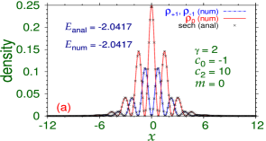
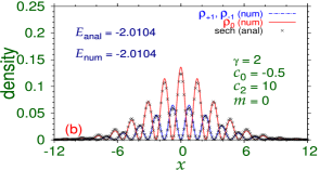
Figure 2: (Color online) Numerical (num) and analytic variational (anal) densities with the secant hyperbolic (sech) function $\rho_{j}(x)\equiv|\phi_{j}|^{2},j=0,\pm 1$ of the three components for the lowest-energy vector soliton with $\gamma=2$, $c_{2}=10,m=0$, for (a) $c_{0}=-1,$ (b) $c_{0}=-0.5$.

We begin our calculation with parameters $c_{0}=-1$ and $c_{2}=10$ ($>0$, polar), to make the system attractive to have a vector soliton of a reasonable width (not too large or small) with magnetization $m=0$. A larger value of $|c_{0}|$ will increase attraction and reduce the width and vice versa, viz. Eq. (44). In Figs. 1(a)-(c) we display the density of the components of the minimum-energy ground-state vector soliton for $\gamma=0.5,1,$ and 5, respectively. The result of the analytic variational approximation with the hyperbolic secant function (50) is also displayed in these plots. In Fig. 1(a) and (b) we also show the analytic result with the Gaussian function (46). In these plots we note, as expected, the analytic approximation with the secant hyperbolic function is better than the that with the Gaussian function. Hence we will show in the following only the analytic result using the secant hyperbolic function. The variational result for the width $\alpha$ given by (44) is the same for all components. The same is found to be true in the numerical calculation, in good agreement with the analytic approximation. Apart from the component densities $\rho_{j}(x)$, we also exhibit in these plots the total numerical density $\rho(x)=\sum_{j}\rho_{j}(x)$ in excellent agreement with the analytic result obtained with the secant hyperbolic function (not shown in these plots). The component densities have pronounced maxima and minima controlled by the functions $\cos^{2}(\gamma x)$ and $\sin^{2}(\gamma x)$, viz. Eqs. (32) or (40). In Fig. 1(c) 14 such maxima are noted. However, the total density $\rho(x)$ has a localized secant hyperbolic (or Gaussian) shape without any maximum or minimum. In Figs. 1(a) the $j=0$ component has a maximum at the center like a bright soliton and the $j=\pm 1$ components have a minimum at the center like a dark soliton. Hence the vector soliton in this plot is of the type dark-bright-dark. The same is true in Fig. 1(b), although in the latter case an undulating tail in component densities starts to appear due to a larger value of the SO coupling strength $\gamma$. In this terminology the vector soliton in Fig. 1(c) with pronounced undulating tails can be termed of the type bright-dark-bright because in this case central maxima in components $j=\pm 1$ is accompanied by a central minimum in component $j=0$. These two types of vector solitons $-$ dark-bright-dark and bright-dark-bright $-$ are degenerate corresponding to the same energy eigenvalue.

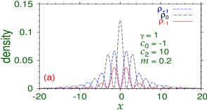
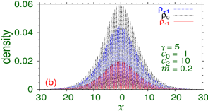
Figure 3: (Color online) Numerical (num) density $\rho_{j}(x)\equiv|\phi_{j}|^{2},j=0,\pm 1$ of the three components for the lowest-energy vector soliton with $c_{0}=-1,c_{2}=10,m=0.2$, for (a) $\gamma=1,$ and (b) $\gamma=5$.

In Figs. 1 we exhibited the pattern of vector solitons for different SO coupling strengths $\gamma$ and find that the number of peaks in the soliton density increases with $\gamma$. In Figs. 2 we show the effect of a variation of the interaction strength $c_{0}$ on the soliton profile. In Figs. 2 we display the soliton profile for $\gamma=2,m=0,c_{2}=10$ and for (a) $c_{0}=-1$ and (b) $c_{0}=-0.5$. A reduced value of $|c_{0}|$ corresponds to reduced attraction resulting in a soliton in Fig. 1(b) with larger spatial extension. In Figs. 1 we see that a increased value of $\gamma$ leads to an increased number of maxima and minima in soliton density due to a larger spatial frequency of undulation. In fact the spatial frequency of density maxima for a wave function profile $\cos(\gamma x)$ or $\sin(\gamma x)$ is $\gamma/\pi$. In Figs. 2 we find that a reduced value of $|c_{0}|$ leads to an increased number of maxima and minima in soliton density due to a larger spatial extension of the vector soliton.

So far we studied the soliton profiles with zero magnetization $m=0$. Next we study these with a non-zero magnetization $m=0.2$. A non-zero magnetization breaks the symmetry between the $j=\pm 1$ states which now will have different spatial densities. For $m=0$ the densities of the $j=\pm 1$ states are the same. In Figs. 3 we display only the numerical density profiles with $c_{0}=-1,c_{2}=10,m=0.2$ and (a) $\gamma=1$ and (b) $\gamma=5$. In this case of non-zero $m$, there is no analytic variational result (valid only for $m=0$). Although the spatial extension of the soliton in Figs. 3(a) and (b) are similar, in the latter case we have many more maxima and minima due to an increased value of $\gamma$ resulting in a larger spatial frequency of density modulation. In Fig. 3(b), for $\gamma=5$, there are more than 60 maxima and minima in density in the spatial range between $x=\pm 20$, the corresponding analytic estimate being $40\times\gamma/\pi\sim 63$ in agreement with the numerical result.

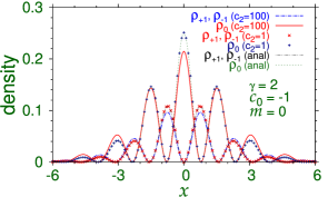
Figure 4: (Color online) Numerical (num) and analytic variational (anal) densities with the secant hyperbolic function $\rho_{j}(x)\equiv|\phi_{j}|^{2},j=0,\pm 1$ of the three components for the lowest-energy vector soliton with $\gamma=2$, $c_{0}=-1,m=0$, for $c_{2}=1,$ and 100. The analytic densities are in agreement with the results for $c_{2}=1$.

We have seen that the analytic results for density and energy of a vector soliton are independent of the interaction strength $c_{2}$ being determined solely by the strength $c_{0}$, viz. Eqs. (49) and (50). The numerical results for density and energy of a vector soliton are not entirely independent of $c_{2}$, they have a weak dependence on $c_{2}$. To demonstrate this, in Fig. 4 we plot the numerical and analytic densities of soliton components for $\gamma=2,c_{0}=-1,m=0$ and for $c_{2}=1$ and 100. The analytic densities are in agreement with the numerical result for $c_{2}=1$ closer to the linear limit where the analytic results are expected to be more reliable.

Now we consider a vector soliton with a very large number of maxima and minima in density with a small $|c_{0}|$ and large $\gamma$. A small $|c_{0}|$ increases the spatial extension while a large $\gamma$ increases the spatial frequency of density modulation of the components of a stripe vector soliton [19]. In Figs. 5(a)-(b) we display the soliton densities for components $j=\pm 1$ and $j=0$, respectively, calculated with $c_{0}=-0.1,c_{2}=10,m=0,\gamma=5$. The total soliton density $\rho$ is also displayed in Fig. 5(b). The analytic densities calculated with the secant hyperbolic function are also shown in these plots. From Figs. 5(a)-(b) we find that the numerical densities are in excellent agreement with their simple analytic approximations. Although the component densities of the vector soliton exhibit a large number of maxima and minima ($>150$), the total density exhibited in Fig. 5(b), as expected, has a smooth behavior without any modulation.

To demonstrate that the stripe vector soliton exhibited in Figs. 5(a)-(b) is dynamically stable, we subject the ground-state vector soliton profile, obtained by imaginary-time simulation, to real-time propagation for a long time after giving a perturbation by changing the strength of the nonlinear interaction $c_{2}$ from 10 to 20 at time $t=0$ maintaining other parameters fixed. The real-time propagation was executed for a total time interval of 100. In Fig. 5(c) we exhibit the density profile of the three components at $t=100$ of the vector soliton at the end of real-time propagation together with the total density $\rho$. In this plot we also show the results for total density $\rho$ obtained in imaginary-time propagation as well as using the analytic approximation with the secant hyperbolic function. The long-time stable propagation of the components of the vector soliton as shown in Fig. 5(c) establishes its dynamical stability.

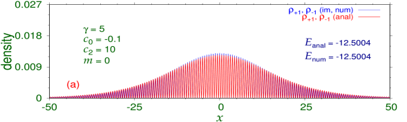
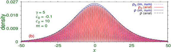
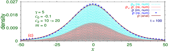
Figure 5: (Color online) (a)-(b) Numerical and analytic variational densities $\rho_{j}$, for (a) $j=\pm 1$ and (b) $j=0$ of the three components of the vector soliton with $c_{0}=-0.1$, $c_{2}=-10$, $\gamma=5,m=0$ by imaginary-time propagation. In (b) we also display the analytic result for $\rho_{0}$ and $\rho$ obtained with the secant hyperbolic function. (c) Results for component and total densities after real-time propagation over an interval of time of 100 units obtained using the converged stationary state of imaginary-time propagation as the initial state after changing $c_{2}$ from 10 to 20 at time $t=0$. The results of total density obtained by imaginary-time propagation and also by analytic approximation are also exhibited.

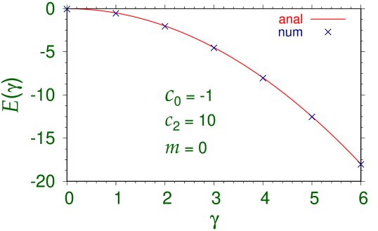
Figure 6: (Color online) Numerical (num) result of energy $E(\gamma)$ of the stationary vector soliton with $c_{0}=-1,c_{2}=10,m=0$ as a function of $\gamma$ compared with the analytic (anal) result $[E(\gamma)=-\gamma^{2}/2-c_{0}/24$] obtained with the secant hyperbolic function, viz. Eq. (49).

Next we test the reliability of the analytic expression for energy of the vector soliton (49) by comparing it with the energies obtained numerically by the imaginary-time propagation method. The result of this study is exposed in Fig. 6, where we display the energy $E(\gamma)$ for different $\gamma$ as obtained numerically and from the analytic approximation (49). The good agreement between the two results is assuring.

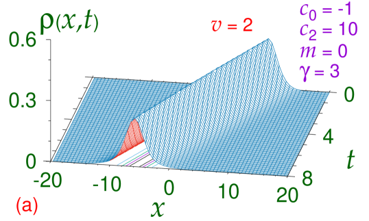
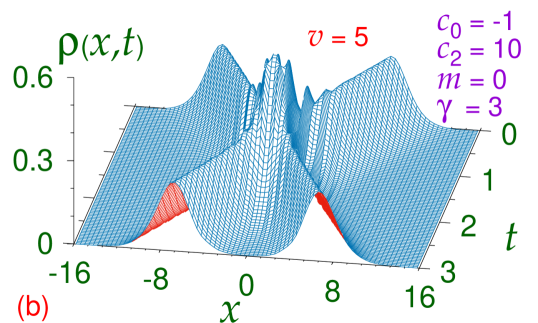
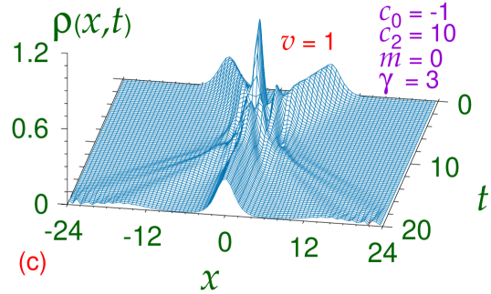
Figure 7: (Color online) (a) Steady propagation by real-time simulation with velocity $v=2$ of a vector soliton preserving its shape. The initial imaginary-time wave function placed at $x=10$ is multiplied by $\exp ivx)$ to start the motion. (b) Elastic nature of collision dynamics of two vector solitons of (a) illustrated through a plot of total density $\rho(x,t)$, obtained by real-time propagation, versus $x$ and $t$. At $t=0$ individual solitons were placed at $x=\pm 8$ and set into motion in opposite directions with velocity $v=\pm 5$, respectively. (c) Inelastic nature of the same dynamics with $v=\pm 1$. Other parameters were $c_{0}=-1,c_{2}=10,m=0,\gamma=3$.

The dynamics of the moving solitons is next studied by first generating a vector soliton numerically using imaginary-time propagation. The complex wave-function components so obtained are then multiplied by a complex phase $\exp(ixv)$, which is used as the initial state in real time simulation to obtain a moving soliton with velocity $v$ in the limit of vanishing small space and time steps $dx$ and $dt$. It is known that the SO-coupled GP equations (6) and (7) are not Galilean invariant [21]. The wave-function ansatz (32) or (40) is a linear combination of two fundamental degenerate solutions of the SO-coupled linear GP equations (9) and (10). In the rest frame $(v=0)$ the physical solution (32) or (40) is constructed as a linear combination of these two fundamental solutions. As the underlying GP equation is not Galilean invariant, for a moving soliton ($v\neq 0$) the two fundamental degenerate solutions will have different energies [21] and one can not consider the same mixture of these two fundamental solutions to construct the same physical solution. Hence the vector soliton cannot move maintaining the same density profile of the component solitons. This will lead to a spin-mixing dynamics during motion with constant change of density profile of the components by a periodic transfer of atoms between components [21], however, preserving the total density profile $\rho(x)$, at least for a reasonable interval of time. First we demonstrate that the vector soliton can move maintaining the total density profile, although the component densities are not conserved. In Fig. 7(a) we show the total density $\rho(x,t)$, obtained by real-time simulation, of the vector soliton with parameters $c_{0}=-1,c_{2}=10,m=0$ and $\gamma=3$ moving with a velocity $v=2$, initially placed at $x=10$. A steady propagation of the vector soliton in this figure is convincing.

To demonstrate the solitonic property of the vector soliton, we study the collision of two vector solitons each generated by imaginary-time propagation with parameters $c_{0}=-1,c_{2}=10,m=0,\gamma=3$. We take two vector solitons and place them at positions $x\equiv d=\pm 8$ and set them in motion in opposite directions with velocity $v=\pm 5$ so as to collide at $x=0$ after time $t=d/v=1.6$. The solitons are found to interact and pass through each other. The total density of each soliton is conserved after collision, showing its elastic nature. This is displayed in Fig. 7(b) via a plot of total density $\rho(x,t)$ of the two solitons during collision. The two solitons emerge with the same velocity and the same total density after collision. However, at a small velocity, the collision of the two solitons turns inelastic. This is exhibited in Fig. 7(c), where we plot the total density of two colliding solitons initially placed at $x=\pm 8$ moving in opposite directions with a velocity $v=\pm 1$. In this case most atoms of the two vector solitons combine to form a larger one which stay at rest at $x=0$ while smaller fractions of atoms move in approximate forward directions. The collision is inelastic with a loss of identity of the two vector solitons. Similar panorama takes place at smaller incident velocities.

4 Summary

We studied the generation, and collision dynamics of three-component $(F_{z}=0,\pm 1)$ 1D vector solitons of a SO-coupled spin-1 polar BEC ($c_{2}>0$) by a numerical solution and an analytic approximation of the mean-field GP equation. The SO coupling is taken as $\gamma p_{x}\Sigma_{y}$, which is an equal-strength mixture of Rashba and Dresselhaus SO couplings [14]. The solitons appear for interaction strength $c_{0}<0$. The vector solitons could have a very large number of maxima and minima. The vector solitons with more than 150 maxima and minima were demonstrated to be stable by real-time propagation during a large interval of time. At large velocities, the collision dynamics between two such vector solitons is found to be elastic with the conservation of the total densities of each individual vector solitons, viz. Fig. 7(b). However, the individual densities of the components are not conserved during collision. The collision with a small velocity is inelastic with the destruction of the individual solitons, viz. Fig. 7(c). A remnant vector soliton soliton molecule appears at rest with lot of dissipation of atoms. With present know-how an experiment can be performed to test the predictions of the present theoretical study.

References

- [1] Y. S. Kivshar and B. A. Malomed, Rev. Mod. Phys. 61, 763 (1989); F. K. Abdullaev, A. Gammal, A. M. Kam- chatnov, and L. Tomio, Int. J. Mod. Phys. B 19, 3415 (2005).
- [2] K. E. Strecker, G. B. Partridge, A. G. Truscott, and R. G. Hulet, Nature (London) 417, 150 (2002); L. Khaykovich, F. Schreck, G. Ferrari, T. Bourdel, J. Cubizolles, L. D. Carr, Y. Castin, and C. Salomon, Science 256, 1290 (2002).
- [3] S. L. Cornish, S. T. Thompson, and C. E. Wieman, Phys. Rev. Lett. 96, 170401 (2006).
- [4] S. Inouye, M. R. Andrews, J. Stenger, H.-J. Miesner, D. M. Stamper-Kurn, and W. Ketterle, Nature (London) 392, 151 (1998).
- [5] V. M. Pérez-García, J. B. Beitia, Phys. Rev. A 72, 033620 (2005); S. K. Adhikari, Phys. Lett. A 346, 179 (2005); L. Salasnich, B. A. Malomed, Phys. Rev. A 74, 053610 (2006).
- [6] V. M. Pérez-García, H. Michinel, H. Herrero, Phys. Rev. A 57, 3837 (1998).
- [7] E. P. Gross, Nuovo Cim. 20, 454 (1961); L.P. Pitaevskii, Sov. Phys. JETP. 13, 451 (1961).
- [8] D. M. Stamper-Kurn, M. R. Andrews, A. P. Chikkatur, S. Inouye, H.-J. Miesner, J. Stenger, W. Ketterle, Phys. Rev. Lett. 80, 2027 (1998).
- [9] Y. Kawaguchi, M. Ueda, Phys. Rep. 520, 253 (2012).
- [10] V. Galitski, I. B. Spielman, Nature (London) 494, 49 (2013); J. Dalibard, F. Gerbier, G. Juzeliūnas, P. Öhberg, Rev. Mod. Phys. 83, 1523 (2011); Y. Li, Giovanni I. Martone, S. Stringari, Ann. Rev. Cold At. Mol. 3, Ch 5, 201 (2015) (World Scientific, 2015).
- [11] K. Osterloh, M. Baig, L. Santos, P. Zoller, M. Lewenstein, Phys. Rev. Lett. 95, 010403 (2005); J. Ruseckas, G. Juzeliūnas, P. Öhberg, M. Fleischhauer, Phys. Rev. Lett. 95, 010404 (2005); G. Juzeliūnas, J. Ruseckas, J. Dalibard, Phys. Rev. A 81, 053403 (2010).
- [12] Y. A. Bychkov E. I. Rashba, J. Phys. C 17, 6039 (1984).
- [13] G. Dresselhaus, Phys. Rev. 100, 580 (1955).
- [14] Y.-J. Lin , K. Jiménez-García, I. B. Spielman, Nature (London) 471, 83 (2011).
- [15] M. Aidelsburger, M. Atala, S. Nascimbène, S. Trotzky, Y.-A. Chen, I. Bloch, Phys. Rev. Lett. 107, 255301 (2011); Z. Fu, P. Wang, S. Chai, L. Huang, J. Zhang, Phys. Rev. A 84, 043609 (2011); J.-Y. Zhang, S.-C. Ji, Z. Chen, L. Zhang, Z.-D. Du, B. Yan, G.-S. Pan, B. Zhao, Y.-J. Deng, H. Zhai, S. Chen, J.-W. Pan, Phys. Rev. Lett. 109, 115301 (2012); C. Qu, C. Hamner, M. Gong, C. Zhang, P. Engels, Phys. Rev. A 88, 021604(R) (2013); A. J. Olson, S.-J. Wang, R. J. Niffenegger, C. -H. Li, C. H. Greene, Y. P. Chen, Phys. Rev. A 90, 013616 (2014).
- [16] Z. Lan, P. Öhberg, Phys. Rev. A 89, 023630 (2014); C. Wang, C. Gao, C.-M. Jian, H. Zhai, Phys. Rev. Lett. 105, 160403 (2010)
- [17] J. Ieda, T. Miyakawa, M. Wadati, Laser Phys. 16, 678 (2006); J. Ieda, T. Miyakawa, M. Wadati, Phys. Rev. Lett. 93, 194102 (2004); L. Li, Z. Li, B. A. Malomed, D. Mihalache, W. M. Liu, Phys. Rev. A 72, 033611 (2005); W. Zhang, Ö. E. Müstecaplioǧlu, L. You, Phys. Rev. A 75, 043601 (2007); B. J. Dabrowska-Wüster, E. A. Ostrovskaya, T. J. Alexander, Y. S. Kivshar, Phys. Rev. A 75, 023617 (2007); E. V. Doktorov, J. Wang, J. Yang, Phys. Rev. A 77, 043617 (2008); B. Xiong, J. Gong; Phys. Rev. A 81, 033618 (2010); P. Szankowski, M. Trippenbach, E. Infeld, G. Rowlands, Phys. Rev. Lett. 105, 125302 (2010); M. Mobarak A. Pelster, Laser Phys. Lett. 10, 115501 (2013); O. Topic, M. Scherer, G. Gebreyesus, et al., Laser Phys. 20, 1156 (2010); M. Guilleumas, B. Julia-Diaz, M. Mele-Messeguer, A. Polls, Laser Phys. 20, 1163 (2010).
- [18] Y. Xu, Y. Zhang, B. Wu, Phys. Rev. A 87, 013614 (2013); S. Cao, C.-J. Shan, D.-W. Zhang, X. Qin, J. Xu, J. Opt. Soc. Am. B 32, 201 (2015); H. Sakaguchi, B. A. Malomed, Phys. Rev. E 90, 062922 (2014); Lin Wen, Q. Sun, Yu Chen, Deng-Shan Wang, J. Hu, H. Chen, W.-M. Liu, G. Juzeliūnas, Boris A. Malomed, An-Chun Ji, Phys. Rev. A 94, 061602(R) (2016).
- [19] V. Achilleos, D. J. Frantzeskakis, P. G. Kevrekidis, D. E. Pelinovsky, Phys. Rev. Lett. 110, 264101 (2013).
- [20] Y.-K. Liu, S.-J. Yang, Europhys. Lett., 108, 30004 (2014); Decheng Ma, Chenglong Jia, Phys. Rev. A 100, 023629 (2019); Yan-Hong Qin, Li-Chen Zhao, Liming Ling, Phys. Rev. E 100, 022212 (2019).
- [21] S. Gautam, S. K. Adhikari, Laser Phys. Lett. 12, 045501 (2015).
- [22] Nian-Sheng Wan, Yu-E Li, Ju-Kui Xue, Phys. Rev. E 99, 062220 (2019); S. Gautam, S. K. Adhikari, Phys. Rev. A 91, 063617 (2015).
- [23] H. Sakaguchi, B. Li, B. A. Malomed, Phys. Rev. E 89, 032920 (2014); S. Gautam, S. K. Adhikari, Phys. Rev. A 95, 013608 (2017); Y. Li, X. Zhang, R. Zhong, Z. Luo, B. Liu, C. Huang, W. Pang, B. A. Malomed, Commun. Nonlinear. Sci. Numer. Simulat. 73, 481 (2019 ; Y. Xu, Y. Zhang, C. Zhang, Phys. Rev. A 92, 013633 (2015).
- [24] S. Gautam, S. K. Adhikari, Phys. Rev. A 97, 013629 (2018); Yong-Chang Zhang, Zheng-Wei Zhou, Boris A. Malomed, Han Pu, Phys. Rev. Lett. 115, 253902 (2015).
- [25] L. Salasnich, A. Parola, L. Reatto, Phys. Rev. A 65, 043614 (2002).
- [26] Y. Li, G. I. Martone, L. P. Pitaevskii, S. Stringari, Phys. Rev. Lett. 110, 235302 (2013); G. I. Martone, Y. Li, L. P. Pitaevskii, S. Stringari, Phys. Rev. A 86, 063621 (2012); Y. Zhang, C. Zhang, Phys. Rev. A 87, 023611 (2013); G. I. Martone, F. V. Pepe, P. Facchi, S. Pascazio, S. Stringari, Phys. Rev. Lett. 117, 125301 (2016).
- [27] F. Y. Lim, W. Bao, Phys. Rev. E 78, 066704 (2008).
- [28] T. Ohmi and K. Machida, J. Phys. Soc. Jap. 67, 1822 (1998); T.-L. Ho, Phys. Rev. Lett. 81, 742 (1998); S. Yi, Ö. E. Müstecaplioǧlu, C. P. Sun, L. You, Phys. Rev. A 66, 011601(R) (2002).
- [29] S. Gautam, S. K. Adhikari, Phys. Rev. A 90, 043619 (2014).
- [30] P. Muruganandam, S. K. Adhikari, Comput. Phys. Commun. 180, 1888 (2009).
- [31] D. Vudragović, I. Vidanović, A. Balaž, P. Muruganandam, S. K. Adhikari, Comput. Phys. Commun. 183, 2021 (2012).
- [32] L. E. Young-S., D. Vudragović, P. Muruganandam, S. K. Adhikari, A. Balaž, Comput. Phys. Commun. 204, 209 (2016); L. E. Young-S., P. Muruganandam, S. K. Adhikari, V. Lončar, D. Vudragović, A. Balaž, Comput. Phys. Commun. 220, 503 (2017); B. Satarić, V. Slavnić, A. Belić, A. Balaž, P. Muruganandam, S. K. Adhikari, Comput. Phys. Commun. 200, 411 (2016).