Data-driven parameterizations of suboptimal LQR and $\mathcal{H}_{2}$ controllers

Abstract

In this paper we design suboptimal control laws for an unknown linear system on the basis of measured data. We focus on the suboptimal linear quadratic regulator problem and the suboptimal $\mathcal{H}_{2}$ control problem. For both problems, we establish conditions under which a given data set contains sufficient information for controller design. We follow up by providing a data-driven parameterization of all suboptimal controllers. We will illustrate our results by numerical simulations, which will reveal an interesting trade-off between the number of collected data samples and the achieved controller performance.

1 Introduction

In the field of systems and control, the majority of control techniques is model-based, meaning that these methods require knowledge of a plant model, for example in the form of a transfer function or state-space system. Such system models are rarely known a priori and typically have to be identified using measured data. The aim of data-driven control is to bypass this system identification step, and to design control laws for dynamical systems directly on the basis of data. Contributions to data-driven control can roughly be divided in on- and offline techniques.

Methods in the former class are iterative and make use of multiple online experiments. Examples include direct adaptive control (Åström and Wittenmark (1989)), iterative feedback tuning (Hjalmarsson et al. (1998)) and methods based on reinforcement learning (Bradtke (1993); Alemzadeh and Mesbahi (2019)). Offline techniques construct controllers on the basis of data (typically a single system trajectory) that is collected offline. Skelton and Shi (1994) consider optimal control using a batch-form solution to the Riccati equation. Virtual reference feedback tuning was introduced by Campi et al. (2002). Moreover, Campestrini et al. (2017) cast the problem of designing model reference controllers in the prediction error framework. Baggio et al. (2019) design minimum energy controls using data. The fundamental lemma by Willems et al. (2005) has also been leveraged for data-driven control in a behavioral setting (Markovsky and Rapisarda (2008)), and in the context of state-space systems to design model predictive controllers (Coulson et al. (2019)), stabilizing and optimal controllers (De Persis and Tesi (2020)) and robust controllers (Berberich et al. (2019)).

An important persisting problem is to understand the relative merits of data-driven control and combined system identification and model-based control, see e.g. (Tu and Recht (2018)). A recent paper sheds some light on this issue by studying data-driven control from the perspective of data informativity. In particular, van Waarde et al. (2020b) provide conditions under which given data contain enough information for control design. For control problems such as stabilization, these conditions do not require that the underlying system can be uniquely identified. As such, one can generally stabilize an unknown system without learning its dynamics exactly. For the linear quadratic regulator problem, however, it was shown that the data essentially need to be rich enough for system identification.

Inspired by the above results, it is our goal to study data-driven suboptimal control problems. Intuitively, we expect that the data requirements for such suboptimal problems are weaker than those for their optimal counterparts. We will focus on data-driven versions of the suboptimal linear quadratic regulator (LQR) problem and the $\mathcal{H}_{2}$ suboptimal control problem. Both of these problems involve the data-guided design of controllers that stabilize the unknown system and render the (LQR or $\mathcal{H}_{2}$) cost smaller than a given tolerance.

Our main results are the following. First, for both suboptimal problems, we establish necessary and sufficient conditions under which the data are informative for control design. These conditions do not require that the underlying system can be identified uniquely. Secondly, for both problems we give a parameterization of all suboptimal controllers in terms of data-driven linear matrix inequalities.

Outline: In §2 we provide some preliminaries. In §3 we state the problem. Next, §4 and §5 contain our main results. An illustrative example is given in §6. Finally, §7 contains our conclusions.

2 Suboptimal control problems

The purpose of this section is to review two (model-based) suboptimal control problems whose data-driven versions will be the main topic of this paper.

2.1 The suboptimal LQR problem

Consider the linear system

$$\bm{x}(t+1)=A\bm{x}(t)+B\bm{u}(t),$$ (1)

where $\bm{x}\in\mathbb{R}^{n}$ is the state, $\bm{u}\in\mathbb{R}^{m}$ is the input and $A$ and $B$ are real matrices of appropriate dimensions. We will occasionally use the shorthand notation $(A,B)$ to refer to system (1). Associated with (1), we consider the infinite-horizon cost functional

$$J(x_{0},u)=\sum_{t=0}^{\infty}x^{\top}(t)Qx(t)+u^{\top}(t)Ru(t),$$ (2)

where $x_{0}$ is the initial state and $Q=Q^{\top}\geqslant 0$ and $R=R^{\top}>0$ are real matrices. Whenever the input function $u$ results from a state feedback law $\bm{u}=K\bm{x}$, we will write $J(x_{0},K)$ instead of $J(x_{0},u)$. The suboptimal linear quadratic regulator problem can be formulated as follows. Given an initial condition $x_{0}\in\mathbb{R}^{n}$ and tolerance $\gamma>0$, find (if it exists) a feedback law $\bm{u}=K\bm{x}$ such that $A+BK$ is stable, and the cost satisfies $J(x_{0},K)<\gamma$. Such a $K$ is called a suboptimal feedback gain for the system $(A,B)$. The following proposition gives necessary and sufficient conditions under which a given matrix $K$ is a suboptimal feedback gain.

Proposition 1

Let $x_{0}\in\mathbb{R}^{n}$ and $\gamma>0$. The matrix $K$ is a suboptimal feedback gain if and only if there exists a matrix $P=P^{\top}>0$ such that

$$(A+BK)^{\top}P(A+BK)-P+Q+K^{\top}RK <0$$ (3)

$$x_{0}^{\top}Px_{0} <\gamma.$$ (4)

2.2 The $\mathcal{H}_{2}$ suboptimal control problem

Consider the system

$$\bm{x}(t+1) =A\bm{x}(t)+B\bm{u}(t)+E\bm{w}(t)$$ (5a)

$$\bm{z}(t) =C\bm{x}(t)+D\bm{u}(t),$$ (5b)

where $\bm{x}\in\mathbb{R}^{n}$ denotes the state, $\bm{u}\in\mathbb{R}^{m}$ is the control input, $\bm{w}\in\mathbb{R}^{d}$ is a disturbance input and $\bm{z}\in\mathbb{R}^{p}$ is the performance output. The real matrices $A,B,C,D$ and $E$ are of appropriate dimensions. The feedback law $\bm{u}=K\bm{x}$ yields the closed-loop system

$$\bm{x}(t+1) =(A+BK)\bm{x}(t)+E\bm{w}(t)$$ (6a)

$$\bm{z}(t) =(C+DK)\bm{x}(t).$$ (6b)

Associated with (6), we consider the $\mathcal{H}_{2}$ cost functional

$$J_{\mathcal{H}_{2}}(K):=\sum_{t=0}^{\infty}\operatorname{tr}\left(T_{K}^{\top}(t)T_{K}(t)\right),$$

where $T_{K}(t):=(C+DK)(A+BK)^{t}E$ is the closed-loop impulse response from $\bm{w}$ to $\bm{z}$ and $\operatorname{tr}$ denotes trace. The cost $J_{\mathcal{H}_{2}}(K)$ equals the squared $\mathcal{H}_{2}$ norm of the transfer function from $\bm{w}$ to $\bm{z}$ of (6). It is well-known that the $\mathcal{H}_{2}$ cost of a given stabilizing $K$ can be computed using the observability Gramian. Indeed for a stabilizing $K$, the unique solution $P$ to the Lyapunov equation

$$(A+BK)^{\top}P(A+BK)-P+(C+DK)^{\top}(C+DK)=0$$ (7)

is related to the $\mathcal{H}_{2}$ cost by $\operatorname{tr}(E^{\top}PE)=J_{\mathcal{H}_{2}}(K)$. For a given $\gamma>0$, the $\mathcal{H}_{2}$ suboptimal control problem amounts to finding a gain $K$ (if it exists) such that $A+BK$ is stable and $J_{\mathcal{H}_{2}}(K)<\gamma$. Such a $K$ is called an $\mathcal{H}_{2}$ suboptimal feedback gain. Similar to Proposition 1 the following proposition gives conditions under which a given $K$ is an $\mathcal{H}_{2}$ suboptimal feedback gain.

Proposition 2

Let $\gamma>0$. The matrix $K$ is an $\mathcal{H}_{2}$ suboptimal feedback gain if and only if there exists a matrix $P=P^{\top}>0$ such that

$$(A+BK)^{\top}P(A+BK)-P+(C+DK)^{\top}(C+DK) <0$$

$$\operatorname{tr}(E^{\top}PE) <\gamma.$$

Clearly, the LQR suboptimal control problem can be viewed as a special case of the $\mathcal{H}_{2}$ suboptimal control problem. Indeed, the $\mathcal{H}_{2}$ problem boils down to the LQR problem if $E=x_{0}$, $C^{\top}C=Q$, $D^{\top}D=R$ and $C^{\top}D=0$. However, as we will see in the next section, the data-driven versions of these problems are different in the way that data is collected.

3 Problem formulation

In this section we formulate our problems. We will start by introducing the data-driven suboptimal LQR problem. Consider the linear system

$$\bm{x}(t+1)=A_{s}\bm{x}(t)+B_{s}\bm{u}(t),$$ (8)

where $\bm{x}\in\mathbb{R}^{n}$ denotes the state, $\bm{u}\in\mathbb{R}^{m}$ is the input and $A_{s}$ and $B_{s}$ are real matrices of appropriate dimensions. We refer to (8) as the ‘true’ system. Suppose that the system matrices $A_{s}$ and $B_{s}$ of the true system are unknown, but we have access to a finite set of data

$$U_{-} :=\begin{bmatrix}u(0)&u(1)&\cdots&u(T-1)\end{bmatrix}$$

$$X_{\phantom{-}} :=\begin{bmatrix}x(0)&x(1)&\cdots&x(T)\end{bmatrix},$$

generated by system (8). By partitioning the state data as

$$X_{-} :=\begin{bmatrix}x(0)&x(1)&\cdots&x(T-1)\end{bmatrix}$$

$$X_{+} :=\begin{bmatrix}x(1)&x(2)&\cdots&x(T)\end{bmatrix},$$

we can relate the data and $(A_{s},B_{s})$ via

$$X_{+}=\begin{bmatrix}A_{s}&B_{s}\end{bmatrix}\begin{bmatrix}X_{-}\\ U_{-}\end{bmatrix}.$$

The set of all systems that explain the input/state data $(U_{-},X)$ is given by

$$\Sigma_{\operatorname{i/s}}:=\left\{(A,B)\mid X_{+}=\begin{bmatrix}A&B\end{bmatrix}\begin{bmatrix}X_{-}\\ U_{-}\end{bmatrix}\right\}.$$

Associated with system (8) we consider the cost functional (2), where the matrices $Q=Q^{\top}\geqslant 0$ and $R=R^{\top}>0$ and the initial condition $x_{0}$ are assumed to be given. We want to design a suboptimal feedback gain for the unknown $(A_{s},B_{s})$ on the basis of the data. Given $(U_{-},X)$, it is impossible to distinguish between the systems in $\Sigma_{\operatorname{i/s}}$, and therefore we can only guarantee that $K$ is a suboptimal gain for $(A_{s},B_{s})$ if it is a suboptimal gain for all systems in $\Sigma_{\operatorname{i/s}}$. With this in mind, we introduce the following notion of data informativity.

Definition 3

Let $x_{0}\in\mathbb{R}^{n}$ and $\gamma>0$. The data $(U_{-},X)$ are informative for suboptimal linear quadratic regulation if there exists a matrix $K$ that is a suboptimal feedback gain for all $(A,B)\in\Sigma_{\operatorname{i/s}}$.

We want to find conditions under which the data are informative for suboptimal LQR, and we want to obtain suboptimal controllers from data. These problems are stated more formally as follows.

Problem 4

Let $x_{0}\in\mathbb{R}^{n}$ and $\gamma>0$. Provide necessary and sufficient conditions under which the data $(U_{-},X)$ are informative for suboptimal linear quadratic regulation. Moreover, for data $(U_{-},X)$ that are informative, find a feedback gain $K$ that is suboptimal for all $(A,B)\in\Sigma_{\operatorname{i/s}}$.

Subsequently, we turn our attention to the $\mathcal{H}_{2}$ suboptimal control problem. For this, consider the system

$$\bm{x}(t+1) =A_{s}\bm{x}(t)+B_{s}\bm{u}(t)+E_{s}\bm{w}(t)$$ (9)

$$\bm{z}(t) =C\bm{x}(t)+D\bm{u}(t),$$ (10)

where the system matrices $A_{s}$, $B_{s}$ and $E_{s}$ are unknown, but the matrices $C$ and $D$ defining the performance output are known. We collect the data $X$ and $U_{-}$ as before, as well as the corresponding measurements of the disturbance

$$W_{-}:=\begin{bmatrix}w(0)&w(1)&\cdots&w(T-1)\end{bmatrix}.$$

The assumption that $W_{-}$ is available is reasonable in applications such as aircraft control, where gust disturbances can be measured via on-board LIDAR measurement systems, see e.g., Soreide et al. (1996). In this setup, all triples of system matrices $(A,B,E)$ that explain the data $(U_{-},W_{-},X)$ are given by

$$\Sigma_{\operatorname{i/d/s}}:=\left\{(A,B,E)\mid X_{+}=\begin{bmatrix}A&B&E\end{bmatrix}\begin{bmatrix}X_{-}\\ U_{-}\\ W_{-}\end{bmatrix}\right\}.$$

We can now state the following notion of data informativity for $\mathcal{H}_{2}$ suboptimal control.

Definition 5

Let $\gamma>0$. The data $(U_{-},W_{-},X)$ are informative for $\mathcal{H}_{2}$ suboptimal control if there exists a $K$ that is an $\mathcal{H}_{2}$ suboptimal feedback gain for all $(A,B,E)\in\Sigma_{\operatorname{i/d/s}}$.

As before, we are interested in both data informativity conditions and a control design procedure. We formalize this in the following problem.

Problem 6

Let $\gamma>0$. Provide necessary and sufficient conditions under which the data $(U_{-},W_{-},X)$ are informative for $\mathcal{H}_{2}$ suboptimal control. Moreover, for data $(U_{-},W_{-},X)$ that are informative, find a feedback gain $K$ that is $\mathcal{H}_{2}$ suboptimal for all $(A,B)\in\Sigma_{\operatorname{i/s}}$.

Remark 7

We note that the data-driven $\mathcal{H}_{2}$ optimal control problem was studied by De Persis and Tesi (2020) in the case that $E_{s}=I$ and $(U_{-},X)$ data are collected in the absence of disturbances. Sufficient data conditions were given for this problem via the concept of persistency of excitation. Moreover, Berberich et al. (2019) aim to design data-driven controllers that minimize a quadratic performance specification (with the $\mathcal{H}_{\infty}$ problem as a special case). The authors provide sufficient data conditions in the scenario that $E$ is known and $\bm{w}$ is unmeasured.

4 Data-driven suboptimal LQR

In this section we report our solution to Problem 4. Before we start, we need some results from (van Waarde et al. (2020b)). We say that $(U_{-},X)$ are informative for stabilization by state feedback if there exists a $K$ such that $A+BK$ is stable for all $(A,B)\in\Sigma_{\operatorname{i/s}}$. The following result was proven in (van Waarde et al., 2020b, Thm. 16).

Lemma 8

The data $(U_{-},X)$ are informative for stabilization by state feedback if and only if there exists a right inverse $X_{-}^{\dagger}$ of $X_{-}$ such that $X_{+}X_{-}^{\dagger}$ is stable.

Moreover, $K$ is a stabilizing feedback for all systems in $\Sigma_{\operatorname{i/s}}$ if and only if $K=U_{-}X_{-}^{\dagger}$ for some $X_{-}^{\dagger}$ satisfying the above properties.

Next, we characterize the informativity of data for suboptimal LQR in terms of data-driven matrix inequalities.

Theorem 9

Let $x_{0}\in\mathbb{R}^{n}$ and $\gamma>0$. The data $(U_{-},X)$ are informative for suboptimal linear quadratic regulation if and only if there exists a matrix $P=P^{\top}>0$ and a right inverse $X_{-}^{\dagger}$ of $X_{-}$ such that

$$(X_{+}X_{-}^{\dagger})^{\top}PX_{+}X_{-}^{\dagger}-P+Q+(U_{-}X_{-}^{\dagger})^{\top}RU_{-}X_{-}^{\dagger} <0$$ (11)

$$x_{0}^{\top}Px_{0} <\gamma.$$ (12)

Moreover, $K$ is a suboptimal feedback gain for all systems $(A,B)\in\Sigma_{\operatorname{i/s}}$ if and only if it is of the form $K=U_{-}X_{-}^{\dagger}$ for some right inverse $X_{-}^{\dagger}$ satisfying (11) and (12).

To prove the ‘if’ parts of both statements, suppose that there exists a matrix $P=P^{\top}>0$ and a right inverse $X_{-}^{\dagger}$ such that (11) and (12) are satisfied. Define the controller $K:=U_{-}X_{-}^{\dagger}$. For any $(A,B)\in\Sigma_{\operatorname{i/s}}$ we have $X_{+}=AX_{-}+BU_{-},$ which implies that $X_{+}X_{-}^{\dagger}=A+BK$. Substitution of the latter expression into (11) yields

$$(A+BK)^{\top}P(A+BK)-P+Q+K^{\top}RK<0,$$

which shows that there exists a $K$ and $P=P^{\top}>0$ satisfying (3) and (4) for all $(A,B)\in\Sigma_{\operatorname{i/s}}$. By Proposition 1, the data are informative for suboptimal LQR.

To prove the ‘only if’ parts of both statements, suppose that the data $(U_{-},X)$ are informative for suboptimal linear quadratic regulation. This means that there exists a feedback gain $K$ and a matrix $P_{(A,B)}=P_{(A,B)}^{\top}>0$ such that

$$(A+BK)^{\top}P_{(A,B)}(A+BK)-P_{(A,B)}+Q+K^{\top}RK <0$$

$$x_{0}^{\top}P_{(A,B)}x_{0} <\gamma$$

for all $(A,B)\in\Sigma_{\operatorname{i/s}}$. We emphasize that the matrix $P_{(A,B)}$ may depend on the particular system $(A,B)$, but the feedback gain $K$ is fixed by definition. Since $K$ is such that $A+BK$ is stable for all $(A,B)\in\Sigma_{\operatorname{i/s}}$, we obtain by Lemma 8 that $K$ is of the form $K=U_{-}X_{-}^{\dagger}$ for some right inverse $X_{-}^{\dagger}$ of $X_{-}$. This yields $A+BK=X_{+}X_{-}^{\dagger}$. The matrix $A+BK$ is therefore the same for all $(A,B)\in\Sigma_{\operatorname{i/s}}$. This implies the existence of a (common) $P=P^{\top}>0$ such that (11) and (12) are satisfied. $\square$

Note that the conditions of Theorem 9 are not ideal from computational point of view since (11) depends nonlinearly on $P$ and $X_{-}^{\dagger}$. Nonetheless, it is straightforward to reformulate these conditions in terms of linear matrix inequalities. This is described in the following corollary.

Corollary 10

Let $Q=C^{\top}C$, $R=D^{\top}D$ and $C^{\top}D=0$, and let $x_{0}\in\mathbb{R}^{n}$ and $\gamma>0$. The data $(U_{-},X)$ are informative for suboptimal linear quadratic regulation if and only if there exist $Y=Y^{\top}\in\mathbb{R}^{n\times n}$ and $\Theta\in\mathbb{R}^{T\times n}$ such that

$$\begin{bmatrix}Y&\Theta^{\top}X_{+}^{\top}&\Theta^{\top}Z_{-}^{\top}\\ X_{+}\Theta&Y&0\\ Z_{-}\Theta&0&I\end{bmatrix} >0$$ (13)

$$\begin{bmatrix}\gamma&x_{0}^{\top}\\ x_{0}&Y\end{bmatrix} >0$$ (14)

$$X_{-}\Theta =Y.$$ (15)

Here $Z_{-}:=CX_{-}+DU_{-}$. Moreover, $K$ is a suboptimal feedback gain for all $(A,B)\in\Sigma_{\operatorname{i/s}}$ if and only if $K=U_{-}\Theta Y^{-1}$ for some $Y$ and $\Theta$ satisfying (13), (14) and (15).

Corollary 10 follows from Theorem 9 via a few well-known tricks, see e.g. Scherer and Weiland (1999). First a congruence transformation $P^{-1}$ is applied to (11), after which a Schur complement argument and change of variables $Y:=P^{-1}$ and $\Theta:=X_{-}^{\dagger}Y$ yields (13), (14) and (15).

Remark 11

It is noteworthy that the conditions of Theorem 9 and Corollary 10 do not require that the data $(U_{-},X)$ contain enough information to uniquely identify the system matrices $(A_{s},B_{s})$. Quite naturally, the conditions do become more difficult to satisfy for decreasing values of $\gamma$. Clearly, Theorem 9 and Corollary 10 require the matrix $X_{-}$ to have full row rank. This means that at least $T\geqslant n$ samples are needed to obtain a suboptimal controller from data. In comparison, note that to uniquely identify $A_{s}$ and $B_{s}$, it is necessary that the rank condition

$$\operatorname{rank}\begin{bmatrix}X_{-}\\ U_{-}\end{bmatrix}=n+m$$

is satisfied, which is only possible if $T\geqslant n+m$. In §6 we will illustrate Corollary 10 in detail by numerical examples.

5 Data-driven $\mathcal{H}_{2}$ suboptimal control

In this section we study the data-driven $\mathcal{H}_{2}$ suboptimal control problem as formulated in Problem 6. As a first step, we extend Lemma 8 to systems with disturbances. We say the data $(U_{-},W_{-},X)$ are informative for stabilization by state feedback if there exists $K$ such that $A+BK$ is stable for all $(A,B,E)\in\Sigma_{\operatorname{i/d/s}}$.

Lemma 12

The data $(U_{-},W_{-},X)$ are informative for stabilization by state feedback if and only if there exists a right inverse $X_{-}^{\dagger}$ of $X_{-}$ with the properties that $X_{+}X_{-}^{\dagger}$ is stable and $W_{-}X_{-}^{\dagger}=0$.

Moreover, $K$ is a stabilizing controller for all systems in $\Sigma_{\operatorname{i/d/s}}$ if and only if $K=U_{-}X_{-}^{\dagger}$, where $X_{-}^{\dagger}$ satisfies the above properties.

The proof follows a similar line as that of (van Waarde et al., 2020b, Thm. 16). To prove the ‘if’ part of both statements, suppose that there exists a right inverse $X_{-}^{\dagger}$ such that $X_{+}X_{-}^{\dagger}$ is stable and $W_{-}X_{-}^{\dagger}=0$. Define $K:=U_{-}X_{-}^{\dagger}$. Then $X_{+}X_{-}^{\dagger}=A+BK$ for all $(A,B,E)\in\Sigma_{\operatorname{i/d/s}}$. Hence $A+BK$ is stable for all $(A,B,E)\in\Sigma_{\operatorname{i/d/s}}$ and $K=U_{-}X_{-}^{\dagger}$ is stabilizing.

To prove the ‘only if’ parts, suppose that the data are informative for stabilization by state feedback. Let $K$ be stabilizing for all systems in $\Sigma_{\operatorname{i/d/s}}$. Define the subspace

$$\Sigma_{\operatorname{i/d/s}}^{0}:=\left\{(A_{0},B_{0},E_{0})\mid 0=\begin{bmatrix}A_{0}&B_{0}&E_{0}\end{bmatrix}\begin{bmatrix}X_{-}\\ U_{-}\\ W_{-}\end{bmatrix}\right\}.$$

The matrix $A+BK+\alpha(A_{0}+B_{0}K)$ is stable for all $\alpha\in\mathbb{R}$ and all $(A_{0},B_{0},E_{0})\in\Sigma_{\operatorname{i/d/s}}^{0}$. Thus we have

$$\rho\left(\frac{1}{\alpha}(A+BK)+A_{0}+B_{0}K\right)\leqslant\frac{1}{\alpha}\quad\forall\>\alpha\geqslant 1,$$

where $\rho(\cdot)$ denotes spectral radius. We take the limit as $\alpha\to\infty$, and conclude by continuity of the spectral radius that $A_{0}+B_{0}K$ is nilpotent for all $(A_{0},B_{0},E_{0})\in\Sigma_{\operatorname{i/d/s}}^{0}$. Note that $(A_{0},B_{0},E_{0})\in\Sigma_{\operatorname{i/d/s}}^{0}$ implies that

$$\left((A_{0}+B_{0}K)^{\top}A_{0},(A_{0}+B_{0}K)^{\top}B_{0},(A_{0}+B_{0}K)^{\top}E_{0}\right)$$

is also a member of $\Sigma_{\operatorname{i/d/s}}^{0}$. This implies that the matrix $(A_{0}+B_{0}K)^{\top}(A_{0}+B_{0}K)$ is nilpotent for all $(A_{0},B_{0},E_{0})$. The only symmetric nilpotent matrix is zero, thus $A_{0}+B_{0}K=0$ for all $(A_{0},B_{0},E_{0})\in\Sigma_{\operatorname{i/d/s}}^{0}$. We conclude that

$$\ker\begin{bmatrix}X_{-}^{\top}&U_{-}^{\top}&W_{-}^{\top}\end{bmatrix}\subseteq\ker\begin{bmatrix}I&K^{\top}&0\end{bmatrix},$$

equivalently,

$$\operatorname{im}\begin{bmatrix}I&K^{\top}&0\end{bmatrix}^{\top}\subseteq\operatorname{im}\begin{bmatrix}X_{-}^{\top}&U_{-}^{\top}&W_{-}^{\top}\end{bmatrix}^{\top}.$$

This means that there exists a right inverse $X_{-}^{\dagger}$ of $X_{-}$ such that $K=U_{-}X_{-}^{\dagger}$ and $W_{-}X_{-}^{\dagger}=0$. Clearly, $X_{+}X_{-}^{\dagger}=A+BK$ for all $(A,B,E)\in\Sigma_{\operatorname{i/d/s}}$, hence $X_{+}X_{-}^{\dagger}$ is stable. $\square$ The following theorem provides necessary and sufficient conditions for data informativity for the $\mathcal{H}_{2}$ problem. It also characterizes all suboptimal controllers in terms of the data. Recall that $Z_{-}$ was defined as $Z_{-}=CX_{-}+DU_{-}$.

Theorem 13

Let $\gamma>0$. The data $(U_{-},W_{-},X)$ are informative for $\mathcal{H}_{2}$ suboptimal control if and only if at least one of the following two conditions is satisfied:

1. There exists a right inverse $X_{-}^{\dagger}$ such that $X_{+}X_{-}^{\dagger}$ is stable and

   $$\begin{bmatrix}W_{-}\\ Z_{-}\end{bmatrix}X_{-}^{\dagger}=0.$$

2. There exist right inverses $X_{-}^{\dagger}$ and $W_{-}^{\dagger}$ such that $X_{+}X_{-}^{\dagger}$ is stable, $W_{-}X_{-}^{\dagger}=0$,

   $$\begin{bmatrix}X_{-}\\ U_{-}\end{bmatrix}W_{-}^{\dagger}=0,$$

   and the unique solution $P$ to

   $$(X_{-}^{\dagger})^{\top}\left(X_{+}^{\top}PX_{+}-X_{-}^{\top}PX_{-}+Z_{-}^{\top}Z_{-}\right)X_{-}^{\dagger}=0$$ (16)

   has the property that

   $$\operatorname{tr}\left((X_{+}W_{-}^{\dagger})^{\top}PX_{+}W_{-}^{\dagger}\right)<\gamma.$$ (17)

Moreover, $K$ is an $\mathcal{H}_{2}$ suboptimal controller for all $(A,B,E)\in\Sigma_{\operatorname{i/d/s}}$ if and only if $K=U_{-}X_{-}^{\dagger}$, where $X_{-}^{\dagger}$ satisfies the conditions of (i) or 17.

Remark 14

The interpretation of Theorem 13 is as follows. Note that both condition (i) and 17 require the existence of $X_{-}^{\dagger}$ such that $X_{+}X_{-}^{\dagger}$ is stable and $W_{-}X_{-}^{\dagger}=0$. These conditions are necessary for the existence of a stabilizing controller by Lemma 12. In condition (i) it is further required that $X_{-}^{\dagger}$ satisfies $Z_{-}X_{-}^{\dagger}=0$, which means that the output of all systems in $\Sigma_{\operatorname{i/d/s}}$ can be made identically equal to zero (hence the $\mathcal{H}_{2}$ norm is zero). In condition 17, the properties of $W_{-}^{\dagger}$ imply that $E_{s}=X_{+}W_{-}^{\dagger}$ can be uniquely identified from the data. Similar to the suboptimal LQR problem, it is generally not required that $A_{s}$ and $B_{s}$ can be uniquely identified from the data.

We first prove the ‘if’ parts of both statements. Suppose that condition (i) is satisfied and let $K:=U_{-}X_{-}^{\dagger}$. By Lemma 12, $A+BK$ is stable for all $(A,B,E)\in\Sigma_{\operatorname{i/d/s}}$. As $Z_{-}X_{-}^{\dagger}=0$ we have $C+DU_{-}X_{-}^{\dagger}=C+DK=0$. This means that the $\mathcal{H}_{2}$ norm of (6) is zero for all $(A,B,E)\in\Sigma_{\operatorname{i/d/s}}$. We conclude that the data are informative for $\mathcal{H}_{2}$ suboptimal control and $K$ is an $\mathcal{H}_{2}$ suboptimal controller.

Next suppose that condition 17 is satisfied, and let $K:=U_{-}X_{-}^{\dagger}$ where $X_{-}^{\dagger}$ satisfies the conditions of 17. Clearly, $A+BK=X_{+}X_{-}^{\dagger}$ is stable for all $(A,B,E)\in\Sigma_{\operatorname{i/d/s}}$. By the properties of $W_{-}^{\dagger}$, $(A,B,E)\in\Sigma_{\operatorname{i/d/s}}$ implies $E=E_{s}$. In view of (16) and (17) we see that for any $(A,B,E_{s})\in\Sigma_{\operatorname{i/d/s}}$ the unique solution $P$ to (7) satisfies $\operatorname{tr}(E_{s}^{\top}PE_{s})<\gamma$. Therefore, the data are informative for $\mathcal{H}_{2}$ suboptimal control and $K$ is $\mathcal{H}_{2}$ suboptimal.

Subsequently, we prove the ‘only if’ parts of both statements. Suppose that the data are informative for $\mathcal{H}_{2}$ suboptimal control and let $K$ be an $\mathcal{H}_{2}$ suboptimal controller for all $(A,B,E)\in\Sigma_{\operatorname{i/d/s}}$. By Lemma 12, there exists a right inverse $X_{-}^{\dagger}$ such that $X_{+}X_{-}^{\dagger}$ is stable and $W_{-}X_{-}^{\dagger}=0$. Also, the feedback $K$ is of the form $K=U_{-}X_{-}^{\dagger}$. The solution $P$ to (16) exists and is unique by stability of $X_{+}X_{-}^{\dagger}$. The matrix $P$ satisfies $\operatorname{tr}(E^{\top}PE)<\gamma$ for all $(A,B,E)\in\Sigma_{\operatorname{i/d/s}}$. Therefore, we have

$$\operatorname{tr}\left((E+\alpha E_{0})^{\top}P(E+\alpha E_{0})\right)<\gamma$$ (18)

for all $(A,B,E)\in\Sigma_{\operatorname{i/d/s}}$, $(A_{0},B_{0},E_{0})\in\Sigma^{0}_{\operatorname{i/d/s}}$ and $\alpha\in\mathbb{R}$. We divide both sides of (18) by $\alpha^{2}$ and take the limit as $\alpha\to\infty$. Then, by continuity of the trace we obtain $\operatorname{tr}(E_{0}^{\top}PE_{0})=0$, which yields $PE_{0}=0$ for all $(A_{0},B_{0},E_{0})\in\Sigma^{0}_{\operatorname{i/d/s}}$. We claim that this implies that either $P=0$ or $E_{0}=0$ for all $(A_{0},B_{0},E_{0})\in\Sigma^{0}_{\operatorname{i/d/s}}$. Suppose that this claim is not true. Then $P\neq 0$ and there exists a triple $(A_{0},B_{0},E_{0})\in\Sigma^{0}_{\operatorname{i/d/s}}$ such that $E_{0}\neq 0$. Note that $(FA_{0},FB_{0},FE_{0})\in\Sigma^{0}_{\operatorname{i/d/s}}$ for any $F\in\mathbb{R}^{n\times n}$. Clearly, there exists an $F$ such that $PFE_{0}\neq 0$. This is a contradiction, which proves our claim. Now, in the case that $P=0$ we obtain $Z_{-}X_{-}^{\dagger}$ and condition (i) is satisfied. In the case that $E_{0}=0$ for all $(A_{0},B_{0},E_{0})\in\Sigma^{0}_{\operatorname{i/d/s}}$, there exists a right inverse $W_{-}^{\dagger}$ such that $X_{-}W_{-}^{\dagger}=0$ and $U_{-}W_{-}^{\dagger}=0$. This means that $(A,B,E)\in\Sigma_{\operatorname{i/d/s}}$ implies $E=E_{s}=X_{+}W_{-}^{\dagger}$. Hence (17), and therefore 17, holds. In both cases, the controller $K$ is of the form $K=U_{-}X_{-}^{\dagger}$, where $X_{-}^{\dagger}$ satisfies either (i) or 17. $\square$ Similar to Corollary 10 we can reformulate Theorem 13 in terms of linear matrix inequalities using Proposition 2.

Corollary 15

Let $\gamma>0$. The data $(U_{-},W_{-},X)$ are informative for $\mathcal{H}_{2}$ suboptimal control if and only if at least one of the following two conditions is satisfied:

1. There exists a $\Theta\in\mathbb{R}^{T\times n}$ such that $X_{-}\Theta=(X_{-}\Theta)^{\top}$,

   $$\begin{bmatrix}W_{-}\\ Z_{-}\end{bmatrix}\Theta=0\text{ and }\begin{bmatrix}X_{-}\Theta&\Theta^{\top}X_{+}^{\top}\\ X_{+}\Theta&X_{-}\Theta\end{bmatrix}>0.$$

2. There exists a right inverse $W_{-}^{\dagger}$, a $Y=Y^{\top}\in\mathbb{R}^{n\times n}$ and $\Theta\in\mathbb{R}^{T\times n}$ such that $X_{-}\Theta$ is symmetric, the matrices $W_{-}\Theta$, $X_{-}W_{-}^{\dagger}$ and $U_{-}W_{-}^{\dagger}$ are zero, and

   $$\begin{bmatrix}X_{-}\Theta&\Theta^{\top}X_{+}^{\top}&\Theta^{\top}Z_{-}^{\top}\\ X_{+}\Theta&X_{-}\Theta&0\\ Z_{-}\Theta&0&I\end{bmatrix} >0$$

   $$\begin{bmatrix}Y&(W_{-}^{\dagger})^{\top}X_{+}^{\top}\\ X_{+}W_{-}^{\dagger}&X_{-}\Theta\end{bmatrix} >0$$

   $$\operatorname{tr}(Y) <\gamma.$$

Moreover, $K$ is an $\mathcal{H}_{2}$ suboptimal controller for all $(A,B,E)\in\Sigma_{\operatorname{i/d/s}}$ if and only if $K=U_{-}\Theta(X_{-}\Theta)^{-1}$, where $\Theta$ satisfies the conditions of (i) or (ii).

6 Illustrative example

We study steered consensus dynamics of the form

$$\bm{x}(t+1)=\left(I-0.15L\right)\bm{x}(t)+B\bm{u}(t),$$ (19)

where $\bm{x}\in\mathbb{R}^{20}$, $\bm{u}\in\mathbb{R}^{10}$, $L$ is the Laplacian matrix of the graph $G$ in Figure 1, and $B=\begin{bmatrix}I&0\end{bmatrix}^{\top}$, meaning that inputs are applied to the first 10 nodes. The goal of this example is to apply the theory from §4 to construct suboptimal controllers for (19) using data. We choose the weight matrices as $Q=I$ and $R=I$, and define $x_{0}\in\mathbb{R}^{20}$ entry-wise as $(x_{0})_{i}=i$.

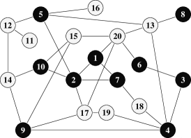
Figure 1: Graph $G$ with leader vertices colored black.

We start with a time horizon of $T=20$ and collect data $(U_{-},X)$ where the entries of $U_{-}$ and the initial state of the experiment $x(0)$ are drawn uniformly at random from $(0,1)$. Given these data, we attempt to solve a semidefinite program (SDP) where the objective is to minimize $\gamma$ subject to the constraints (13), (14) and (15). We use Yalmip, with Mosek as a solver. Next, we collect one additional sample of the input and state, and we solve the SDP again for the augmented data set. We continue this process up to a time horizon of $T=30$.

We repeat this entire experiment for 100 trials and display the results in Figures 2 and 3. Figure 2 depicts the fraction of successful trials in which the constraints (13), (14) and (15) were feasible and a stabilizing controller was found. Note that a stabilizing controller was only found in 2 out of the 100 trials for $T=20$. This fraction rapidly increases to $0.88$ for $T=22$, while $100\%$ of the trials were successful for $T\geqslant 24$. Figure 3 displays the minimum cost $\gamma$ of the controller, averaged over all successful trials. The cost is very large for small sample size $(T=20)$ but decreases rapidly as the number of samples increases. Figure 3 therefore highlights an interesting trade-off between the sample size and the cost. Note that for $T=30$, $\gamma$ coincides with the optimal cost obtained from the (model-based) solution to the Riccati equation. This is as expected since $30=n+m$ is the minimum number of samples from which the state and input matrices can be uniquely identified.

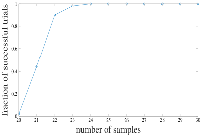
Figure 2: Fraction of successful trials as a function of $T$.

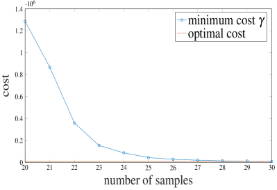
Figure 3: Average minimum cost as a function of $T$.

7 Conclusions

In this paper we have studied the data-driven suboptimal LQR and $\mathcal{H}_{2}$ problems. For both problems, we have presented conditions under which a given data set contains sufficient information for control design. We have also given a parameterization of all suboptimal controllers in terms of data-driven linear matrix inequalities. Finally, we have illustrated these results by numerical simulations, which reveal a trade-off between the number of collected data samples and the achieved controller performance.

References

- Alemzadeh and Mesbahi (2019) Alemzadeh, S. and Mesbahi, M. (2019). Distributed Q-learning for dynamically decoupled systems. In Proceedings of the American Control Conference, 772–777.
- Åström and Wittenmark (1989) Åström, K.J. and Wittenmark, B. (1989). Adaptive Control. Addison-Wesley.
- Baggio et al. (2019) Baggio, G., Katewa, V., and Pasqualetti, F. (2019). Data-driven minimum-energy controls for linear systems. IEEE Control Systems Letters, 3(3), 589–594.
- Berberich et al. (2019) Berberich, J., Romer, A., Scherer, C.W., and Allgöwer, F. (2019). Robust data-driven state-feedback design. https://arxiv.org/pdf/1909.04314v1.pdf.
- Bradtke (1993) Bradtke, S.J. (1993). Reinforcement learning applied to linear quadratic regulation. In Advances in Neural Information Processing Systems, 295–302.
- Campestrini et al. (2017) Campestrini, L., Eckhard, D., Bazanella, A.S., and Gevers, M. (2017). Data-driven model reference control design by prediction error identification. Journal of the Franklin Institute, 354(6), 2628–2647.
- Campi et al. (2002) Campi, M., Lecchini, A., and Savaresi, S. (2002). Virtual reference feedback tuning: a direct method for the design of feedback controllers. Automatica, 38(8), 1337–1346.
- Coulson et al. (2019) Coulson, J., Lygeros, J., and Dörfler, F. (2019). Data-enabled predictive control: In the shallows of the DeePC. In Proceedings of the European Control Conference, 307–312.
- De Persis and Tesi (2020) De Persis, C. and Tesi, P. (2020). Formulas for data-driven control: Stabilization, optimality, and robustness. IEEE Transactions on Automatic Control, 65(3), 909–924.
- Hjalmarsson et al. (1998) Hjalmarsson, H., Gevers, M., Gunnarsson, S., and Lequin, O. (1998). Iterative feedback tuning: theory and applications. IEEE Control Systems Magazine, 18(4), 26–41.
- Markovsky and Rapisarda (2008) Markovsky, I. and Rapisarda, P. (2008). Data-driven simulation and control. International Journal of Control, 81(12), 1946–1959.
- Scherer and Weiland (1999) Scherer, C.W. and Weiland, S. (1999). Lecture notes DISC course on linear matrix inequalities in control.
- Skelton and Shi (1994) Skelton, R.E. and Shi, G. (1994). The data-based LQG control problem. In Proceedings of the IEEE Conference on Decision and Control, 1447–1452.
- Soreide et al. (1996) Soreide, D.C., Bogue, R.K., Ehernberger, L.J., and Bagley, H.R. (1996). Coherent lidar turbulence for gust load alleviation. In Optical Instruments for Weather Forecasting, volume 2832, 61–75. International Society for Optics and Photonics.
- Tu and Recht (2018) Tu, S. and Recht, B. (2018). The gap between model-based and model-free methods on the linear quadratic regulator: An asymptotic viewpoint. https://arxiv.org/abs/1812.03565.
- van Waarde et al. (2020a) van Waarde, H.J., De Persis, C., Camlibel, M.K., and Tesi, P. (2020a). Willems’ fundamental lemma for state-space systems and its extension to multiple datasets. IEEE Control Systems Letters, 4(3), 602–607.
- van Waarde et al. (2020b) van Waarde, H.J., Eising, J., Trentelman, H.L., and Camlibel, M.K. (2020b). Data informativity: a new perspective on data-driven analysis and control. IEEE Transactions on Automatic Control, to appear.
- Willems et al. (2005) Willems, J.C., Rapisarda, P., Markovsky, I., and De Moor, B.L.M. (2005). A note on persistency of excitation. Systems & Control Letters, 54(4), 325–329.