On privacy preserving data release of linear dynamic networks

Abstract

Distributed data sharing in dynamic networks is ubiquitous. It raises the concern that the private information of dynamic networks could be leaked when data receivers are malicious or communication channels are insecure. In this paper, we propose to intentionally perturb the inputs and outputs of a linear dynamic system to protect the privacy of target initial states and inputs from released outputs. We formulate the problem of perturbation design as an optimization problem which minimizes the cost caused by the added perturbations while maintaining system controllability and ensuring the privacy. We analyze the computational complexity of the formulated optimization problem. To minimize the $\ell_{0}$ and $\ell_{2}$ norms of the added perturbations, we derive their convex relaxations which can be efficiently solved. The efficacy of the proposed techniques is verified by a case study on a heating, ventilation, and air conditioning system.

,

1 Introduction

Recently, information and communications technologies are increasingly integrated with control systems in the physical world. It has been stimulating the rapid emergence of cyber-physical systems (CPS). CPS consists of a large number of geographically dispersed entities and thus distributed data sharing is necessary to achieve network-wide goals. However, distributed data sharing also raises the significant concern that the private or confidential information of legitimate entities could be leaked to malicious entities. Privacy has become an issue of high priority to address before certain CPS can be widely deployed. For example, the current absence of accepted solutions to tackle privacy concerns caused a deadlock in the mandatory deployment of smart meters in the Netherlands because of the common belief that smart metering is necessarily privacy-invasive (Cavoukian, 2012). In 2010, California’s new law on smart meter privacy indicated strong demands to protect the privacy of end-users’ energy consumption data (California Public Utilities Commission, 2010).

In the security community, several notions have been used to define privacy. In particular, differentially private schemes add random noises into each individual’s data in such a way that, with high probability, the participation of the individual cannot be inferred by an adversary, who can access arbitrary auxiliary information, via released data (Dwork and Roth, 2014). Mutual information (Sankar et al., 2013) requires explicit statistical models of source data and auxiliary/side information and quantifies average uncertainties about source data conditioned on revealed data. Semantic security (Goldwasser and Micali, 1984) requires that no additional information about a plaintext can be inferred using its ciphertext by any probabilistic polynomial-time algorithm. Perfect secrecy (Shannon, 1949) is stronger than semantic security in that it assumes that the adversary has unlimited computing power. Additionally, $k$-anonymity (Samarati and Sweeney, 1998) protects identity privacy by requiring that each group of records that share the same values for the quasi-identifiers (e.g., age, gender, zip code) must include at least $k$ records. The notion of $\ell$-diversity (Machanavajjhala et al., 2007) extends $k$-anonymity to protect attribute privacy by requiring that there is adequate diversity in each sensitive attribute. The notion of $t$-closeness (Li et al., 2007) further refines $\ell$-diversity by taking into account side information of a priori distributions of the attributes.

In the control and CPS communities, differential privacy has been adopted to Kalman filtering (Le Ny and Pappas, 2014), consensus (Huang et al., 2012) and optimization (Nozari et al., 2016; Zhang et al., 2016); mutual information has been used as a privacy metric in the applications of smart grid (Han et al., 2016) and stochastic control systems (Venkitasubramaniam et al., 2015); semantic security and perfect secrecy have been employed in secure multiparty computation (Lu and Zhu, 2015) and homomorphic encryption (Lu and Zhu, 2018).

Contributions. This paper considers a linear dynamic network where a set of agents are physically coupled. An external data requester requires the agents to release system outputs in real time. The agents aim to prevent the data requester from inferring initial states and past inputs through the released outputs. We define that the privacy is protected if the data requester has infinite uncertainty on each of its target entries after observing the released outputs. Our uncertainty-based privacy notion extends $\ell$-diversity from the discrete-valued setting to the continuous-valued setting. Please refer to Section 2.3 and the appendix for the justification of our privacy definition. We propose a protection scheme where the agents intentionally perturb the inputs and outputs such that (i) privacy is protected; (ii) system controllability is maintained; and (iii) the cost induced by the perturbations is minimized. We investigate two cases of the cost function:
(1) The sparsity of the perturbations is maximized, i.e., the $\ell_{0}$ norm of the added perturbations is minimized.
(2) The utility of the released outputs is maximized, i.e., the $\ell_{2}$ norm of the added perturbations is minimized.

We first analyze the computational complexity of the formulated optimization problem. We then derive a semidefinite program relaxation for the $\ell_{0}$ norm minimization by adopting the $\ell_{1}$ norm heuristic, the nuclear norm heuristic and a positive semidefinite condition. For the $\ell_{2}$ norm minimization, by using the tool of singular value decomposition, we provide a computationally more efficient method which can return an analytic feasible solution. Finally, the efficacy of the developed techniques is verified by a case study on a heating, ventilation, and air conditioning (HVAC) system.

A preliminary version of this paper is presented in (Zhu and Lu, 2015). Compared with (Zhu and Lu, 2015), in the current paper, the privacy definition is refined; a thorough analysis of computational complexity is provided; the relaxation for the $\ell_{0}$ minimization problem is developed; the $\ell_{2}$ minimization is extended to allow for general rank deficiency constraints; a case study on an HVAC system is provided.

Notations and notions. For any $k\in\mathbb{N}$, denote by $x_{[0,k]}$ the sequence of $\{x_{0},\cdots,x_{k}\}$. The induced $\ell_{1}$ norm, $\ell_{2}$ norm and Frobenius norm of matrix $M$ are denoted by $\|M\|_{1}$, $\|M\|_{2}$ and $\|M\|_{F}$, respectively. $\|M\|_{0}$ denotes the number of nonzero entries of matrix $M$ and is referred to as its $\ell_{0}$ norm. $\|M\|_{*}$ denotes the sum of the singular values of matrix $M$ and is referred to as its nuclear norm. For a column vector $w\in\mathbb{R}^{n}$, define a quantity $|\cdot|_{\min}$ as $|w|_{\min}=\min_{\ell\in\{1,\cdots,n\}}|w_{\ell}|$. $\mathbb{S}^{n}$ denotes the set of real symmetric matrices of size $n$. Denote by $M^{\dagger}$ and $M^{-1}$ the pseudo inverse and inverse of matrix $M$, respectively. The notation $M=[M_{ij}]$ means that $M$ is a matrix for which the entry at the position of the $i$-th row and the $j$-th column is $M_{ij}$, or the $ij$-th block is $M_{ij}$ if $M_{ij}$ itself is a matrix. For a vector $x$, $x=[x_{i}]$ means that the $i$-th entry of $x$ is $x_{i}$. ${\rm Tr}(M)$, ${\rm rank}(M)$ and ${\rm det}(M)$ denote the trace, the rank and the determinant of matrix $M$, respectively. Given a matrix $M$, denote by ${\rm vec}(M)$ the column vector consisting of the entries of $M$. $\textbf{0}_{n}$ is the column vector with $n$ zeros. $\textbf{0}_{m\times n}$ denotes the $m\times n$ matrix where all entries are zeros. $I_{n}$ denotes the identity matrix of size $n$. In computational complexity, a polynomial-time algorithm is an algorithm performing its task in a number of steps bounded by a polynomial expression in the size of the problem input. NP (nondeterministic polynomial time), one of the most fundamental complexity classes, is the set of decision problems where the “yes”-instances can be accepted in polynomial time by a nondeterministic Turing machine. A decision problem $\mathcal{D}$ is NP-hard if for every problem $\mathcal{D}^{\prime}$ in NP, there is a polynomial-time reduction from $\mathcal{D}^{\prime}$ to $\mathcal{D}$ (Leeuwen, 1990).

2 Problem Statement

This section introduces the system model, the adversary model and the privacy notion adopted in this paper.

2.1 Network model

Consider an interconnected dynamic network of $V=\{1,\cdots,N\}$ where the physical dynamics of agent $i$ are described by the following linear discrete-time system:

$$x_{i}(k+1) =\bar{A}_{ii}x_{i}(k)+\sum\nolimits_{j\in\mathcal{N}_{i}}\bar{A}_{ij}x_{j}(k)+\bar{B}_{i}u_{i}(k)$$

$$y_{i}^{\prime}(k) =\bar{G}_{i}^{\prime}x_{i}(k)+\bar{H}_{i}^{\prime}u_{i}(k).$$ (1)

In (1), $x_{i}(k)\in\mathbb{R}^{n_{i}}$, $u_{i}(k)\in\mathbb{R}^{p_{i}}$ and $y_{i}^{\prime}(k)\in\mathbb{R}^{l_{i}}$ are the state, input and output of agent $i$ at time instant $k$, respectively, and $\mathcal{N}_{i}\subseteq V\setminus\{i\}$ is the set of agents whose states affect the state of agent $i$. The collection of states and outputs in (1) can be compactly written as follows:

$$x(k+1) =\bar{A}x(k)+\bar{B}u(k)$$ (2)

$$y^{\prime}(k) =\bar{G}^{\prime}x(k)+\bar{H}^{\prime}u(k)$$ (3)

where $x(k)=[x_{i}(k)]\in\mathbb{R}^{n}$, $u(k)=[u_{i}(k)]\in\mathbb{R}^{p}$ and $y^{\prime}(k)=[y_{i}^{\prime}(k)]\in\mathbb{R}^{l}$, with $n=\sum_{i\in V}n_{i}$, $p=\sum_{i\in V}p_{i}$ and $l=\sum_{i\in V}l_{i}$. The matrices $\bar{A}$, $\bar{B}$, $\bar{G}^{\prime}$ and $\bar{H}^{\prime}$ are system parameters known to the agents. In this paper, we assume that each agent is allowed to communicate with any other agent and measure all the entries of its own state. The activation of a communication link or a sensor induces certain cost.

2.2 Adversary model

There is an external data requester who requests a set of linear combinations of the agents’ individual outputs. Specifically, the data requester determines a constant matrix $\Pi\in\mathbb{R}^{q\times l}$ and tells its valuation to a data aggregator. Each agent $i$ measures its output $y_{i}^{\prime}(k)$ and sends it to the data aggregator, who then computes $y(k)=\Pi y^{\prime}(k)$ and sends $y(k)$ to the data requester. Hence, the data received by the data requester is:

$$y(k)=\Pi y^{\prime}(k)=\bar{G}x(k)+\bar{H}u(k)$$ (4)

where $\bar{G}=\Pi\bar{G}^{\prime}\in\mathbb{R}^{q\times n}$ and $\bar{H}=\Pi\bar{H}^{\prime}\in\mathbb{R}^{q\times p}$. The agents are unaware of how the released data will be used. In the rest of the paper, we use $(A,B,G,H)$ to represent arbitrary system matrices, while $(\bar{A},\bar{B},\bar{G},\bar{H})$ specifically represent system (2) and (4).

The data requester is assumed to be semi-honest (Lindell and Pinkas, 2009), and aims to exploit $y(k)$ to infer some entries of $x(0)$ and $\{u(k)\}$. Our problem model is motivated by several practical scenarios, e.g., smart building and load monitoring in smart grid. For both of these two applications, the physical dynamics can be approximated by a linear dynamic model (Kang et al., 2014; Maruta and Takarada, 2014). In smart building, a system operator (data requester) uses temperature data of individual rooms (agents) to monitor working comfortability and energy usage conditions. At the same time, it may aim to infer occupancy data from room temperature information, and by the occupancy data, it might be able to derive the location traces of individual occupants (Lisovich et al., 2010). In smart grid, a utility company (data requester) collects power consumption data stored at local smart meters of power consumers (agents) to monitor power usage conditions. Meanwhile, it may target to infer power load profiles of individual consumers from aggregated home power consumption information (McLaughlin et al., 2011).We assume that the data requester is aware of the matrices $\bar{A}$, $\bar{B}$, $\bar{G}^{\prime}$ and $\bar{H}^{\prime}$. This assumption models the auxiliary/side information of the adversary. In this paper, we assume that all the agents in $V$ and the data aggregator are benign, i.e., they will not use their observed information to infer other agents’ private data.

2.3 Privacy notion

We next introduce the privacy notion adopted in this paper. The data requester aims to infer the values of partial (could be all) entries of the initial state $x(0)$ and the input sequence $\{u(k)\}$. We call those entries as target entries. The remaining entries of $x(0)$ and $\{u(k)\}$ are called nontarget entries. Denote by $x^{t}(0)$ and $x^{n}(0)$ (resp. $u^{t}$ and $u^{n}$) the column vectors of the target and nontarget entries of $x(0)$ (resp. $u$), respectively. Denote by $d_{x}^{t}$, $d_{u}^{t}$, $d_{x}^{n}$ and $d_{u}^{n}$ the dimensions of $x^{t}(0)$, $u^{t}$, $x^{n}(0)$ and $u^{n}$, respectively. It holds that $d_{x}^{t}+d_{x}^{n}=n$ and $d_{u}^{t}+d_{u}^{n}=p$. Denote by $x_{\ell}^{t}(0)$ (resp. $u_{\ell}^{t}$, $x_{\ell}^{n}(0)$ and $u_{\ell}^{n}$) the $\ell$-th entry of $x^{t}(0)$ (resp. $u^{t}$, $x^{n}(0)$ and $u^{n}$). For a target entry $u_{\ell}^{t}$, we consider that it is protected if and only if $u_{\ell}^{t}(k)$ is protected for any $k\in\mathbb{N}$. In other words, if the value of $u_{\ell}^{t}(k)$ for one time instant $k$ is disclosed to the data requester, then we consider that the privacy of $u_{\ell}^{t}$ is compromised.

Given system matrices $(A,B,G,H)$, for each time instant $k$, the output $y(k)$ can be expressed as a linear combination of the entries of $x(0)$ and $u_{[0,k]}$:

$$\!\!\!y(k)=GA^{k}x(0)+\sum\limits_{m=0}^{k-1}GA^{k-1-m}Bu(m)+Hu(k).$$ (5)

Given system matrices $(A,B,G,H)$ and time instant $\kappa\in\mathbb{N}$, for any feasible output sequence $y_{[0,\kappa]}$, we define a set $\Delta_{A,B,G,H}(y_{[0,\kappa]})$ as:

$$\Delta_{A,B,G,H}(y_{[0,\kappa]})=\{x^{t}(0),u^{t}_{[0,\kappa]}:\exists x^{n}(0),u^{n}_{[0,\kappa]},$$

$${\rm s.t.}\;y(k)={\rm right\text{-}hand\text{-}side\;of}\;\eqref{standard output relation},\forall k=0,\cdots,\kappa,$$

$${\rm with}\;x(0)\;{\rm the\;composition\;of\;}x^{t}(0)\;{\rm and}\;x^{n}(0)\;{\rm and}\;u(k)$$

$${\rm the\;composition\;of}\;u^{t}(k)\;{\rm and}\;u^{n}(k),\forall k=0,\cdots,\kappa\}.$$

The set $\Delta_{A,B,G,H}(y_{[0,\kappa]})$ includes all possible valuations of $\{x^{t}(0),u^{t}_{[0,\kappa]}\}$ that can generate $y_{[0,\kappa]}$ in (5). We define the diameter of $\Delta_{A,B,G,H}(y_{[0,\kappa]})$ as:

$${\rm Diam}_{A,B,G,H}(y_{[0,\kappa]})=\sup\limits_{w,w^{\prime}\in\Delta_{A,B,G,H}(y_{[0,\kappa]})}|w-w^{\prime}|_{\min}.$$

Definition 2.1.

Given system matrices $(A,B,G,H)$, the privacy of $x^{t}(0)$ and $u^{t}$ is said to be protected if, for any $\kappa\in\mathbb{N}$, ${\rm Diam}_{A,B,G,H}(y_{[0,\kappa]})=\infty$ for any feasible output sequence $y_{[0,\kappa]}$. $\bullet$

We next justify Definition 2.1 through comparisons with several popular existing notions in our problem setting.

$\bullet$ Why not semantic security or perfect secrecy? These notions require that “nothing is learned” by the adversary from outputs. However, as pointed out in Section 2.2 of (Dwork and Roth, 2014), such “nothing is learned” definition cannot be adopted to applications in which the outputs have to be used to realize certain utility by the data user who is adversary, because such a strong privacy requirement intrinsically inhibits any meaningful data utility. In our problem, the adversary and the data user is the same entity, i.e., the data requester, and it has to accomplish certain analysis using the outputs.

$\bullet$ Why not mutual information metric? The usage of mutual information metric requires explicit statistical models of source data and auxiliary/side information (Sankar et al., 2013). This requirement might be restrictive or even unrealistic for our problem as the inputs of the system may not follow any probabilistic distribution.

$\bullet$ Why not differential privacy? To achieve differential privacy, noises are persistently added to the released data via following, e.g., Gaussian and Laplace distributions. For control systems, such open-loop and persistent noise injection mechanisms could potentially deteriorate system performance.

$\bullet$ Our uncertainty-based privacy notion Definition 2.1. Definition 2.1 is extended from the notion of $\ell$-diversity. In particular, $\ell$-diversity has been widely used in both application-centric research (Kumar and Karthikeyan, 2012; Li and Das, 2013) and formal privacy analysis (Last et al., 2014; Li et al., 2007) on attribute privacy of discrete-valued tabular datasets. Besides academic studies, $k$-anonymity and $\ell$-diversity have also been popular in real world applications. As mentioned in page 16 of (Malle et al., 2017), $k$-anonymity has become a standard privacy notion in the industry. For example, the password manager 1Password has applied $k$-anonymity to protect the privacy of the customers’ passwords (Brodkin, 2018). Recently, Google released a data loss prevention application programming interface (API) which supported $k$-anonymity and $\ell$-diversity (Hopping, 2017).

Informally speaking, possessing $\ell$-diversity means that there are at least $\ell$ different values for each sensitive attribute of the dataset in the released table. A larger diversity indicates a larger uncertainty and thus the notion of diversity can be viewed as a measure of uncertainty. To make an analogy to $\ell$-diversity, in our problem, we can view each entry of $x^{t}(0)$ and $u^{t}$ as a sensitive attribute and require adequate diversity/uncertainty on it. In $\ell$-diversity, the diversity of discrete-valued sensitive attributes is defined by the number of different valuations for the attributes. In contrast, the target entries $x^{t}(0)$ and $u^{t}$ in our problem are continuous-valued and uncountable, which requires a new measure to quantify the diversity/uncertainty. In this paper, given system matrices $(A,B,G,H)$, the diversity/uncertainty is measured by the diameter of the set $\Delta_{A,B,G,H}(y_{[0,\kappa]})$. Hence, Definition 2.1 extends the notion of $\ell$-diversity from the discrete-valued setting to the continuous-valued setting. A detailed introduction to $\ell$-diversity and extension to Definition 2.1 in our problem setting is given in the appendix.

Definition 2.1 is closely relevant to non-strong observability (Hautus, 1983) in control theory. Specifically, a dynamic system is not strongly observable if at least one entry of the initial states and input sequence is unobservable, i.e., cannot be uniquely determined. However, non-strong observability does not necessarily imply that all the target entries are unobservable. Definition 2.1 extends non-strong observability by explicitly ensuring such property. Using the language of control theory, Definition 2.1 can be equivalently stated as follows: Given system matrices $(A,B,G,H)$, the privacy of the target entries is said to be protected if no target entry is in the strongly observable subspace of system $(A,B,G,H)$. This uncertainty/unobservability-based privacy definition has been widely adopted in the control community; please see, e.g., (Mo and Murray, 2017) and (Pequito et al., 2014), in which the initial state of a system is private if it is not in the observable subspace.

In discrete event systems, the notion of opacity has been widely used to define system state privacy (Wu and Lafortune, 2014; Ramasubramanian et al., 2016; Ji et al., 2018). A system is opaque if for every secret-induced behavior, there exists a non-secret-induced behavior that generates identical observations. The notion of opacity is similar to our privacy notion in spirit. However, the privacy objectives are different. In opacity-based works, the privacy objective is to ensure that the adversary cannot determine from the observations whether or not the system state belongs to a predefined secret set. In contrast, Definition 2.1 aims to protect data privacy such that for any valuation of any target entry, the adversary has infinite uncertainty from the observations on the value of the target entry.

Advantages. Compared with semantic security and perfect secrecy, our notion is weaker than the “nothing is learned” requirement and allows for meaningful data utility. Compared with mutual information, our notion does not require any statistical model for system states, inputs and outputs. Compared with differential privacy, our notion does not require using persistent perturbations. Please refer to Remark 3.1 for more discussions.

Limitation. A limitation of our privacy notion is that it does not take into account the scenario where the data requester has auxiliary information of some a priori skewed distribution of $x(0)$ and $\{u(k)\}$. Note that $\ell$-diversity is also vulnerable to skewness attacks (Li et al., 2007). For this case, instead of requiring infinite uncertainty on the target data items, the privacy goal should be that the posterior uncertainties after seeing the observations should be as close as possible to the a priori uncertainties determined by the a priori skewed distribution. This privacy goal extends $t$-closeness (Li et al., 2007), which is a refinement of $\ell$-diversity, from discrete-valued settings to continuous-valued settings. We leave the study of the refined privacy goal as a future work.

2.4 Privacy preserving data release

To protect privacy, we propose to perturb the inputs and outputs such that the data requester cannot infer the target entries in the sense of Definition 2.1. However, the perturbations should maintain certain system utilities, e.g., controllability. Throughout this paper, we assume that the original system $(\bar{A},\bar{B})$ is controllable and aim to maintain controllability of the perturbed system. These partially conflicting sub-objectives define the problem of privacy preserving data release. In the remainder of the paper, we introduce our solutions of this problem. First, in Section 3, we introduce our perturbation mechanism and the optimization formulation to solve for the optimal perturbation. In particular, we formulate an $\ell_{0}$ optimization that studies economy-privacy tradeoff and an $\ell_{2}$ optimization that studies utility-privacy tradeoff. After that, we show that the formulated optimization problems are hard to solve. In Section 4, we first provide a further computational complexity result for the $\ell_{0}$ optimization problem and then derive a convex relaxation for it. A convex relaxation for the $\ell_{2}$ optimization problem is derived in Section 5.

3 Intentional input-output perturbations

In this section, we first introduce a class of optimization problems to formulate intentional input-output perturbations. After that, we analyze the computational complexity of the formulated optimization problem.

3.1 Optimization formulation

To protect privacy, we propose the approach of intentional input-output perturbations. Each agent $i$ intentionally perturbs its own input $u_{i}(k)$ and output $y_{i}^{\prime}(k)$ by adding signals $\mu_{i}^{\mu}(k)\in\mathbb{R}^{p_{i}}$ and $\mu_{i}^{y}(k)\in\mathbb{R}^{l_{i}}$, respectively. The perturbations $\mu_{i}^{u}(k)$ and $\mu_{i}^{y}(k)$ are linear combinations of system states and inputs and given by:

$$\mu_{i}^{u}(k) =\sum\nolimits_{j\in V}K_{ij}^{SS}x_{j}(k)+\sum\nolimits_{j\in V}K_{ij}^{SI}u_{j}(k)$$

$$\mu_{i}^{y}(k) =\sum\nolimits_{j\in V}K_{ij}^{OS}x_{j}(k)+\sum\nolimits_{j\in V}K_{ij}^{OI}u_{j}(k).$$ (6)

The superscript $SI$ means a perturbation from an input to a state. Other superscripts are defined analogously, with $O$ denoting output. Substituting the perturbations $\mu^{u}(k)=[\mu_{i}^{u}(k)]$ and $\mu^{y}(k)=[\mu_{i}^{y}(k)]$ into (2) and (4) renders the following perturbed system:

$$x(k+1) =\bar{A}x(k)+\bar{B}(u(k)+\mu^{u}(k))$$

$$=\hat{A}x(k)+\hat{B}u(k)$$ (7)

$$y(k) =\Pi(\bar{G}^{\prime}x(k)+\bar{H}^{\prime}(u(k)+\mu^{u}(k))+\mu^{y}(k))$$

$$=\hat{G}x(k)+\hat{H}u(k)$$ (8)

where $\hat{A}=\bar{A}+\bar{B}K_{SS}$, $\hat{B}=\bar{B}(I_{p}+K_{SI})$, $\hat{G}=\bar{G}+\bar{H}K_{SS}+\Pi K_{OS}$ and $\hat{H}=\bar{H}+\bar{H}K_{SI}+\Pi K_{OI}$, with $K_{SS}=[K_{ij}^{SS}]\in\mathbb{R}^{p\times n}$, $K_{SI}=[K_{ij}^{SI}]\in\mathbb{R}^{p\times p}$, $K_{OS}=[K_{ij}^{OS}]\in\mathbb{R}^{l\times n}$ and $K_{OI}=[K_{ij}^{OI}]\in\mathbb{R}^{l\times p}$. Let $K=\left[\begin{array}[]{cc}K_{SS}&K_{SI}\\ K_{OS}&K_{OI}\end{array}\right]\in\mathbb{R}^{(p+l)\times(n+p)}$. In the rest of the paper, we use $(\hat{A},\hat{B},\hat{G},\hat{H})$ to specifically represent the perturbed system (3.1) and (3.1). The perturbation matrix $K$ is subject to two constraints:
(i) The perturbed system $(\hat{A},\hat{B})$ remains controllable.
(ii) The data requester cannot infer the target entries in the sense of Definition 2.1 from the outputs (3.1).

By adding $\mu^{u}$ to $u$ according to (6), the perturbed input $\hat{u}$ is $\hat{u}=u+\mu^{u}=K_{SS}x+(I_{p}+K_{SI})u$ and this actually changes system matrices $(\bar{A},\bar{B})$ to $(\hat{A},\hat{B})$. The controllability of $(\bar{A},\bar{B})$ does not guarantee that of $(\hat{A},\hat{B})$. Denote by ${\mathcal{C}}(K_{SS},K_{SI})$ the controllability matrix of the perturbed system, i.e.,
${\mathcal{C}}(K_{SS},K_{SI})=[\hat{B},\hat{A}\hat{B},\cdots,\hat{A}^{n-1}\hat{B}]\\ =[\bar{B}(I_{p}+K_{SI}),(\bar{A}+\bar{B}K_{SS})\bar{B}(I_{p}+K_{SI}),\\ \quad\;\cdots,(\bar{A}+\bar{B}K_{SS})^{n-1}\bar{B}(I_{p}+K_{SI})]$.
The perturbed system is controllable if and only if ${\rm det}({\mathcal{C}}(K_{SS},K_{SI})({\mathcal{C}}(K_{SS},K_{SI}))^{T})$ $>0$. Meanwhile, the agents aim to minimize the cost induced by the perturbations. This is captured by minimizing an objective function $c(K)$ determined later. All the above objectives are encoded in the following optimization problem:

$$\min\nolimits_{K\in\mathbb{R}^{(p+l)\times(n+p)}}c(K)$$

$${\rm s.t.}\,{\rm Diam}_{\hat{A},\hat{B},\hat{G},\hat{H}}(y_{[0,\kappa]})=\infty,\forall\kappa\in\mathbb{N}\;{\rm and}\;{\rm feasible}\;y_{[0,\kappa]},$$

$$\quad\;\;{\rm det}({\mathcal{C}}(K_{SS},K_{SI})({\mathcal{C}}(K_{SS},K_{SI}))^{T})>0.$$ (9)

In this paper, we study the following two representative cases of the cost function.

Problem $\mathbb{P}_{0}$: economy–privacy tradeoff. The added perturbations require communication and sensing. If one entry of $K^{SS}_{ji}$ or $K^{OS}_{ji}$ is nonzero, then agent $i$ needs to measure the corresponding entry of $x_{i}$ and sends it to agent $j$. If one entry of of $K^{SI}_{ji}$ or $K^{OI}_{ji}$ is nonzero, then agent $i$ needs to share its control $u_{i}$ with agent $j$. Recall that activation of communication links and sensors induces some cost. Minimizing such cost can be encoded into maximizing the sparsity of the perturbation matrix $K$ and equivalently minimizing the $\ell_{0}$ norm of $K$, i.e., $c(K)=\|K\|_{0}$ in problem (3.1). This is referred to as the $\ell_{0}$ minimization and denoted by $\mathbb{P}_{0}$.

Problem $\mathbb{P}_{2}$: utility–privacy tradeoff. The goal of the data requester is to collect the true output. In this paper setup, the true output $y(k)$ is the linear combination of $x(k)$ and $u(k)$ weighted by the original output matrices $(\bar{G},\bar{H})$, i.e., $\bar{G}x(k)+\bar{H}u(k)$. The difference between the released output $y(k)$ of (3.1) and the true output $\bar{G}x(k)+\bar{H}u(k)$ is data disutility. Notice that the perturbation added into the state equation (2) does not change the linear combination and thus does not affect data disutility. Instead, these perturbations can protect the privacy of target entries. We rewrite (3.1) as $y(k)=\bar{G}x(k)+\bar{H}u(k)+[\bar{H},\Pi]K[x(k)^{T},u(k)^{T}]^{T}$ and define data disutility as $\left\|[\bar{H},\Pi]K[x(k)^{T},u(k)^{T}]^{T}\right\|_{2}$. Notice that $\left\|[\bar{H},\Pi]K[x(k)^{T},u(k)^{T}]^{T}\right\|_{2}\leq\left\|[\bar{H},\Pi]K\right\|_{2}$ $\left\|[x(k)^{T},u(k)^{T}]^{T}\right\|_{2}$, and $x(k)$ and $u(k)$ are not decision variables. Hence, we turn to minimize $\left\|[\bar{H},\Pi]K\right\|_{2}$, i.e., $c(K)=\left\|[\bar{H},\Pi]K\right\|_{2}$ in problem (3.1). This is referred to as the $\ell_{2}$ minimization and denoted by $\mathbb{P}_{2}$.

We assume that the optimal perturbation matrix $K$, i.e., the solution of problem (3.1), is known to the data requester. This is another piece of auxiliary information available to the data requester.

Remark 3.1.

Similar to differential privacy, our technique also adopts perturbations for privacy preservation. However, by (6), it can be seen that the perturbations are added in a closed-loop fashion and diminishing as the system is stabilized. Since we formulate problem (3.1) such that the perturbed system remains controllable, one can design a feedback controller by the perturbed system matrices $(\bar{A}+\bar{B}K_{SS},\bar{B}(I_{p}+K_{SI}))$ to achieve perfect stability where the perturbations vanish at the equilibrium.

Data privacy has a fundamental utility-privacy tradeoff: disclosing fully accurate information maximizes data utility but minimizes data privacy, while disclosing random noises achieves the opposite (Li and Li, 2009). Our optimization formulation (3.1) utilizes control theory to characterize the tradeoff. This allows us to take into account dynamic system utilities, e.g., controllability, which have not been addressed in the literature. $\bullet$

3.2 Relaxation of problem (3.1)

The first constraint of (3.1) has a clear privacy interpretation, but is not analytically tractable. In this subsection, we identify a relation between the privacy constraint and the rank deficiency of a matrix pencil, which allows us to relax the privacy constraint by a rank constraint.

Given a linear system $(A,B,G,H)$, for any $z\in\mathbb{C}$, define matrix pencil
$D_{A,B,G,H}(z)=\left[\begin{array}[]{cc}zI_{n}-A&-B\\ G&H\\ \end{array}\right]$.
For any $v\in\mathbb{R}^{n+p}$, we write $v=[v_{1}^{T},v_{2}^{T}]^{T}$ with $v_{1}\in\mathbb{R}^{n}$ and $v_{2}\in\mathbb{R}^{p}$. Let $v_{1}^{t}$ (resp. $v_{2}^{t}$) be the sub-vector of $v_{1}$ (resp. $v_{2}$) corresponding to $x^{t}(0)$ (resp. $u^{t}$), i.e., if the $\ell$-th entry of $x(0)$ (resp. $u$) is an entry of $x^{t}(0)$ (resp. $u^{t}$), then the $\ell$-th entry of $v_{1}$ (resp. $v_{2}$) is an entry of $v_{1}^{t}$ (resp. $v_{2}^{t}$). The dimensions of $v_{1}^{t}$ and $v_{2}^{t}$ are then $d_{x}^{t}$ and $d_{u}^{t}$, respectively. Denote by $v_{1\ell}^{t}$ (resp. $v_{2\ell}^{t}$) the $\ell$-th entry of $v_{1}^{t}$ (resp. $v_{2}^{t}$).

The following lemma provides a sufficient condition for privacy protection. Its proof leverages properties of the matrix pencil defined above, and closely follows and extends the rank-based characterizations of strong observability (Hautus, 1983; Kratz, 1995).

Lemma 3.1.

Given a linear system $(A,B,G,H)$, the privacy of $x^{t}(0)$ and $u^{t}$ is protected if there exists a pair of $z\in\mathbb{C}$ and $v\in\mathbb{R}^{n+p}\backslash\{\textbf{0}_{n+p}\}$ satisfying $D_{A,B,G,H}(z)v=\textbf{0}_{n+q}$ such that the following two conditions are satisfied simultaneously:
(1) if $d_{x}^{t}\neq 0$, then $v_{1\ell}^{t}\neq 0$ for all $\ell\in\{1,\cdots,d_{x}^{t}\}$;
(2) if $d_{u}^{t}\neq 0$, then $z\neq 0$ and $v_{2\ell}^{t}\neq 0$ for all $\ell\in\{1,\cdots,d_{u}^{t}\}$. $\bullet$

Proof: Given that $D_{A,B,G,H}(z)v=\textbf{0}_{n+q}$, we have $Av_{1}+Bv_{2}=zv_{1}$ and $Gv_{1}+Hv_{2}=0_{q}$. Fix any $\kappa\in\mathbb{N}$ and any feasible output sequence $y_{[0,\kappa]}$. Denote by $x(0)^{\prime}$ and $u_{[0,\kappa]}{{}^{\prime}}$ an arbitrary set of initial states and input sequence that satisfy $y_{[0,\kappa]}$, i.e., $x(k+1)^{\prime}=Ax(k)^{\prime}+Bu(k)^{\prime}$ and $y(k)=Gx(k)^{\prime}+Hu(k)^{\prime}$ for any $k\in\{0,\cdots,\kappa\}$. We then have $\{x^{t}(0)^{\prime},u^{t}_{[0,\kappa]}{{}^{\prime}}\}\in\Delta_{A,B,G,H}(y_{[0,\kappa]})$. Denote $x(0)^{\prime\prime}=x(0)^{\prime}+mv_{1}$ and $u(k)^{\prime\prime}=u(k)^{\prime}+mz^{k}v_{2}$ for each $k\in\{0,\cdots,\kappa\}$, where $m$ is an arbitrary scalar. We next show by mathematical induction that, with the initial state $x(0)^{\prime\prime}$ and input sequence $u_{[0,\kappa]}{{}^{\prime\prime}}$, $x(k)^{\prime\prime}=x(k)^{\prime}+mz^{k}v_{1}$ for any $k\in\{0,\cdots,\kappa\}$. For $k=0$, we have $x(0)^{\prime\prime}=x(0)^{\prime}+mv_{1}=x(0)^{\prime}+mz^{0}v_{1}$. For $k=1$, we have
$x(1)^{\prime\prime}=Ax(0)^{\prime\prime}+Bu(0)^{\prime\prime}\\ =A(x(0)^{\prime}+mv_{1})+B(u(0)^{\prime}+mv_{2})\\ =Ax(0)^{\prime}+Bu(0)^{\prime}+m(Av_{1}+Bv_{2})=x(1)^{\prime}+mzv_{1}$. Assume that $x(k)^{\prime\prime}=x(k)^{\prime}+mz^{k}v_{1}$. Then, we have
$x(k+1)^{\prime\prime}=Ax(k)^{\prime\prime}+Bu(k)^{\prime\prime}\\ =A(x(k)^{\prime}+mz^{k}v_{1})+B(u(k)^{\prime}+mz^{k}v_{2})\\ =Ax(k)^{\prime}+Bu(k)^{\prime}+mz^{k}(Av_{1}+Bv_{2})\\ =x(k+1)^{\prime}+mz^{k+1}v_{1}$.
We then have $x(k)^{\prime\prime}=x(k)^{\prime}+mz^{k}v_{1}$ for any $k\in\{0,\cdots,\kappa\}$. Hence, for any $k\in\{0,\cdots,\kappa\}$, we have
$Gx(k)^{\prime\prime}+Hu(k)^{\prime\prime}\\ =G(x(k)^{\prime}+mz^{k}v_{1})+H(u(k)^{\prime}+mz^{k}v_{2})\\ =Gx(k)^{\prime}+Hu(k)^{\prime}+mz^{k}(Gv_{1}+Hv_{2})\\ =Gx(k)^{\prime}+Hu(k)^{\prime}=y(k)$.
This implies $\{x^{t}(0)^{\prime\prime},u^{t}_{[0,\kappa]}{{}^{\prime\prime}}\}\in\Delta_{A,B,G,H}(y_{[0,\kappa]})$. Note
$\min_{\ell\in\{1,\cdots,d_{x}^{t}\}}|x_{\ell}^{t}(0)^{\prime}-x_{\ell}^{t}(0)^{\prime\prime}|=\min_{\ell\in\{1,\cdots,d_{x}^{t}\}}|mv_{1\ell}^{t}|,\\ \min_{\scriptstyle\ell\in\{1,\cdots,d_{u}^{t}\}\hfill\atop\scriptstyle k\in\{0,\cdots,\kappa\}\hfill}|u_{\ell}^{t}(k)^{\prime}-u_{\ell}^{t}(k)^{\prime\prime}|=\min_{\scriptstyle\ell\in\{1,\cdots,d_{u}^{t}\}\hfill\atop\scriptstyle k\in\{0,\cdots,\kappa\}\hfill}|mz^{k}v_{2\ell}^{t}|$.
If $v_{1\ell}^{t}\neq 0$ $\forall\ell\in\{1,\cdots,d_{x}^{t}\}$ and $v_{2\ell}^{t}\neq 0$ $\forall\ell\in\{1,\cdots,d_{u}^{t}\}$ and $z\neq 0$, then
${\rm Diam}_{A,B,G,H}(y_{[0,\kappa]})\geq\\ \sup\limits_{m\in\mathbb{R}}\min\{\min\limits_{\ell\in\{1,\cdots,d_{x}^{t}\}}|mv_{1\ell}^{t}|,\min\limits_{\scriptstyle\ell\in\{1,\cdots,d_{u}^{t}\}\hfill\atop\scriptstyle k\in\{0,\cdots,\kappa\}\hfill}|mz^{k}v_{2\ell}^{t}|\}=\infty$. The above analysis holds for any $\kappa\in\mathbb{N}$ and any feasible $y_{[0,\kappa]}$. By Definition 2.1, $x^{t}(0)$ and $u^{t}$ are protected. $\bullet$

Lemma 3.1 requires that the matrix pencil $D_{A,B,G,H}(z)$ does not have full column rank. Intuitively, one can protect more entries of $x(0)$ and $u$ by reducing the rank of $D_{A,B,G,H}(z)$. This is verified by the following lemma.

Lemma 3.2.

Given $(A,B,G,H)$, if there exists $z\neq 0$ such that $D_{A,B,G,H}(z)$ has column rank $r$, then at least $n+p-r$ entries of $x(0)$ and $u$ can be protected. $\bullet$

Proof: If $D_{A,B,G,H}(z)$ has column rank $r$, then the null space of $D_{A,B,G,H}(z)$ has rank $n+p-r$. This implies that $D_{A,B,G,H}(z)$ must have a null vector $v$ with at least $n+p-r$ non-zero entries. By Lemma 3.1, at least $n+p-r$ entries of $x(0)$ and $u$ are protected. $\bullet$

For convenience of notation, in the rest of the paper, let $\bar{D}(z)=D_{\bar{A},\bar{B},\bar{G},\bar{H}}(z)$ and $\hat{D}(z)=D_{\hat{A},\hat{B},\hat{G},\hat{H}}(z)$, i.e., $\bar{D}(z)$ and $\hat{D}(z)$ are the matrix pencils of the original system $(\bar{A},\bar{B},\bar{G},\bar{H})$ and the perturbed system $(\hat{A},\hat{B},\hat{G},\hat{H})$, respectively. It can be checked that $\hat{D}(z)=\bar{D}(z)+FK$ with $F=\left[\begin{array}[]{cc}-\bar{B}&\textbf{0}_{n\times l}\\ \bar{H}&\Pi\\ \end{array}\right]$. Lemma 3.2 states that one can protect more entries of $x(0)$ and $u$ by reducing the rank of $\hat{D}(z)$. With more entries of $x(0)$ and $u$ being protected, in general, it is more likely that more entries of $x^{t}(0)$ and $u^{t}$ can be protected. By this observation, we relax problem (3.1) as follows:

$$\min\nolimits_{K\in\mathbb{R}^{(p+l)\times(n+p)},z\in\mathbb{C}}c(K)$$

$${\rm s.t.}\;{\rm rank}(\bar{D}(z)+FK)<\rho,$$

$$\quad\;\;{\rm det}({\mathcal{C}}(K_{SS},K_{SI})({\mathcal{C}}(K_{SS},K_{SI}))^{T})>0$$ (10)

where $\rho\in[1,\min\{n+p,n+q\}]$ is a constant integer. In the remaining, we use $\tilde{\mathbb{P}}_{0}$ (resp. $\tilde{\mathbb{P}}_{2}$) to denote problem (3.2) with $c(K)=\|K\|_{0}$ (resp. $c(K)=\left\|[\bar{H},\Pi]K\right\|_{2}$).

Given any integer $\rho$ between $[1,\min\{n+p,n+q\}]$, by Lemma 3.2, the optimal solution of problem (3.2) can guarantee that at least $n+p-\rho+1$ entries of $x(0)$ and $u$ can be protected in the perturbed system. However, Lemma 3.2 does not indicate which entries of $x(0)$ and $u$ can be protected. We will provide a scheme to perform the verification in the next paragraph. If some entries of $x^{t}(0)$ and $u^{t}$ are not protected, we decrease the value of $\rho$ and re-solve problem (3.2). Our objective is to protect all the entries of $x^{t}(0)$ and $u^{t}$ with the largest possible $\rho$ (so that with the smallest possible perturbation).

We next illustrate a mechanism for checking which entries can be protected in the perturbed system after solving problem (3.2) under a given $\rho$. Given the system matrices $(\bar{A},\bar{B},\bar{G},\bar{H})$ of the original system and an optimal solution $(K,z)$ of problem (3.2), one can derive the null space of $\bar{D}(z)+FK$ and then make use of Lemma 3.1 to check which entries can be protected in the perturbed system. In particular, if the null space of $\bar{D}(z)+FK$ admits a null vector $v=[v_{1}^{T},v_{2}^{T}]^{T}$ such that $v_{1\ell}^{t}\neq 0$, then the $\ell$-th entry of $x^{t}(0)$ is protected. If $z\neq 0$ and the null space of $\bar{D}(z)+FK$ admits a null vector $v$ such that $v_{2\ell}^{t}\neq 0$, then the $\ell$-th entry of $u^{t}$ is protected.

The remaining issue is how to solve problem (3.2) under a given $\rho$. The next theorem shows the non-convexity of the constraint set of problem (3.2), indicating that the problem could be hard to solve and needs to be further relaxed. In the next section, we furhter prove a NP-hardness result for problem $\tilde{\mathbb{P}}_{0}$.

Theorem 3.1.

The constraint set of problem (3.2) is non-convex. $\bullet$

Proof: Denote the constraint set of (3.2) by $\Upsilon$. Let $(z^{\prime},K^{\prime})\in\Upsilon$ be any feasible quadruple. The feasibility implies that ${\mathcal{C}}(K_{SS}^{\prime},K_{SI}^{\prime})$ has full row rank and ${\rm rank}(\bar{D}(z^{\prime})+FK^{\prime})<\rho$. Consider $(K_{SS}^{\prime\prime},K_{SI}^{\prime\prime},K_{OS}^{\prime\prime},K_{OI}^{\prime\prime})$ $=(K_{SS}^{\prime},-K_{SI}^{\prime}-2I_{p},K_{OS}^{\prime},-K_{OI}^{\prime})$. Then
${\mathcal{C}}(K_{SS}^{\prime\prime},K_{SI}^{\prime\prime})={\mathcal{C}}(K_{SS}^{\prime},-K_{SI}^{\prime}-2I_{p})\\ =[\bar{B}(I_{p}-K_{SI}^{\prime}-2I_{p}),(\bar{A}+\bar{B}K_{SS}^{\prime})\bar{B}(I_{p}-K_{SI}^{\prime}-2I_{p}),\\ \cdots,(\bar{A}+\bar{B}K_{SS}^{\prime})^{n-1}\bar{B}(I_{p}-K_{SI}^{\prime}-2I_{p})]\\ =-{\mathcal{C}}(K_{SS}^{\prime},K_{SI}^{\prime})$
which has full row rank. Thus, $(K_{SS}^{\prime\prime},$ $K_{SI}^{\prime\prime})$ satisfies the controllability constraint. Take $z^{\prime\prime}=z^{\prime}$. We have
$\bar{D}(z^{\prime\prime})+FK^{\prime\prime}\\ =\left[\begin{array}[]{cc}z^{\prime\prime}I_{n}-(\bar{A}+\bar{B}K_{SS}^{\prime\prime})&-\bar{B}(I_{p}+K_{SI}^{\prime\prime})\\ \bar{G}+\bar{H}K_{SS}^{\prime\prime}+\Pi K_{OS}^{\prime\prime}&\bar{H}+\bar{H}K_{SI}^{\prime\prime}+\Pi K_{OI}^{\prime\prime}\\ \end{array}\right]\\ =\left[\begin{array}[]{cc}z^{\prime}I_{n}-(\bar{A}+\bar{B}K_{SS}^{\prime})&\bar{B}(I_{p}+K_{SI}^{\prime})\\ \bar{G}+\bar{H}K_{SS}^{\prime}+\Pi K_{OS}^{\prime}&-(\bar{H}+\bar{H}K_{SI}^{\prime}+\Pi K_{OI}^{\prime})\\ \end{array}\right]$
which implies ${\rm rank}(\bar{D}(z^{\prime\prime})+FK^{\prime\prime})={\rm rank}(\bar{D}(z^{\prime})+FK^{\prime})<\rho$. Thus, $(z^{\prime\prime},K^{\prime\prime})\in\Upsilon$.

Now consider another quadruple $(K_{SS}^{\circ},K_{SI}^{\circ},K_{OS}^{\circ},K_{OI}^{\circ})$ $=(K_{SS}^{\prime},-I_{p},K_{OS}^{\prime},\textbf{0}_{l\times p})$. Notice that $(K_{SS}^{\circ},K_{SI}^{\circ},K_{OS}^{\circ},$ $K_{OI}^{\circ})=(K_{SS}^{\prime},-I_{p},K_{OS}^{\prime},\textbf{0}_{l\times p})=\frac{1}{2}(K_{SS}^{\prime},K_{SI}^{\prime},K_{OS}^{\prime},$ $K_{OI}^{\prime})+\frac{1}{2}(K_{SS}^{\prime\prime},K_{SI}^{\prime\prime},K_{OS}^{\prime\prime},K_{OI}^{\prime\prime})$, which implies that $(K_{SS}^{\circ},K_{SI}^{\circ},K_{OS}^{\circ},K_{OI}^{\circ})$ is a convex combination of $(K_{SS}^{\prime},K_{SI}^{\prime},K_{OS}^{\prime},K_{OI}^{\prime})$ and $(K_{SS}^{\prime\prime},K_{SI}^{\prime\prime},$ $K_{OS}^{\prime\prime},K_{OI}^{\prime\prime})$. Let $z^{\circ}=z^{\prime}$. Then $(z^{\circ},K^{\circ})$ is a convex combination of $(z^{\prime},K^{\prime})$ and $(z^{\prime\prime},K^{\prime\prime})$. We have
${\mathcal{C}}(K_{SS}^{\circ},K_{SI}^{\circ})={\mathcal{C}}(K_{SS}^{\prime},-I_{p})\\ =[\bar{B}(I_{p}-I_{p}),(\bar{A}+\bar{B}K_{SS}^{\prime})\bar{B}(I_{p}-I_{p}),\cdots,\\ \quad\;(\bar{A}+\bar{B}K_{SS}^{\prime})^{n-1}\bar{B}(I_{p}-I_{p})]=\textbf{0}_{n\times np}$,
which does not have full row rank. Thus, $(K_{SS}^{\circ},K_{SI}^{\circ})$ does not satisfy the controllability constraint and hence $(z^{\circ},K^{\circ})\notin\Upsilon$. This implies that $\Upsilon$ is non-convex. $\bullet$

4 Problem $\tilde{\mathbb{P}}_{0}$

In this section, we first prove that a relaxation of problem $\tilde{\mathbb{P}}_{0}$ is NP-hard, which indicates that problem $\tilde{\mathbb{P}}_{0}$ itself might also be NP-hard. We then provide a convex approximation for problem $\tilde{\mathbb{P}}_{0}$. Specifically, in problem (3.2), the $\ell_{0}$ norm in the objective function is relaxed by the $\ell_{1}$ norm heuristic, the rank constraint is relaxed by the nuclear norm heuristic, and the controllability constraint is approximated by a symmetric positive semidefinite condition.

4.1 Computational intractability

To obtain a rigorous NP-hardness result, we consider the following problem derived by fixing some $z$ and $[K_{SS},K_{SI}]=\textbf{0}_{p\times(n+p)}$, and dropping the controllability constraint of problem $\tilde{\mathbb{P}}_{0}$:

$$\min\nolimits_{K_{O}\in\mathbb{R}^{l\times(n+p)}}\|K_{O}\|_{0}$$

$${\rm s.t.}\;\;{\rm rank}(\bar{D}(z)+F\left[{\begin{array}[]{*{20}{c}}{{\textbf{0}_{p\times(n+p)}}}\\ {{K_{O}}}\end{array}}\right])<\rho.$$ (13)

where $K_{O}=[K_{OS},K_{OI}]$. Denote problem (4.1) by $\hat{\mathbb{P}}_{0}(z)$. By fixing $z$ and $[K_{SS},K_{SI}]$, the dimension of the decision variables is reduced. By the proof of Theorem 3.1, the controllability constraint of problem $\tilde{\mathbb{P}}_{0}$ is non-convex. Hence, intuitively, problem $\tilde{\mathbb{P}}_{0}$ might be harder to solve than problem $\hat{\mathbb{P}}_{0}(z)$. We next show that problem $\hat{\mathbb{P}}_{0}(z)$ is NP-hard due to the non-convexity of its objective function. This provides an implication that problem $\tilde{\mathbb{P}}_{0}$ might also be NP-hard. We leave the proof of NP-hardness of problem $\tilde{\mathbb{P}}_{0}$ to our future works.

It is well-known that $\ell_{0}$ norm is non-convex and $\ell_{0}$ norm optimization problems are hard to solve in general. However, there has been a limited number of $\ell_{0}$ norm optimization problems which have been rigorously proven to be NP-hard. The following theorem establishes the NP-hardness of problem $\hat{\mathbb{P}}_{0}(z)$ by showing that it is as hard as finding a sparsest null vector of a matrix with more columns than rows, which has been proven to be NP-hard (Coleman and Pothen, 1986).

Theorem 4.1.

Problem $\hat{\mathbb{P}}_{0}(z)$ is NP-hard. $\bullet$

Proof: We prove the NP-hardness of problem $\hat{\mathbb{P}}_{0}(z)$ by following the standard procedure of proving NP-hardness (Leeuwen, 1990):
Step 1. Reduce any instance of a known NP-hard problem to an instance of problem $\hat{\mathbb{P}}_{0}(z)$ in polynomial time;
Step 2. Show that a solution of the instance of the known NP-hard problem can be constructed from a solution of the instance of problem $\hat{\mathbb{P}}_{0}(z)$ in polynomial time.

The known NP-hard problem we use is the following null vector problem (NVP) (Coleman and Pothen, 1986):

Null vector problem: Given a matrix $M\in\mathbb{R}^{r\times c}$ with $r<c$, find a sparest null vector of $M$, i.e., find an optimal solution $v^{*}$ to the following optimization problem

$$\min\nolimits_{v\in\mathbb{R}^{c}\backslash\{\textbf{0}_{c}\}}\|v\|_{0}\quad{\rm s.t.}\;\;Mv=\textbf{0}_{r}.$$ (14)

Step 1. Consider a matrix $M\in\mathbb{R}^{r\times c}$ with $r<c$. Let $M=[M_{1},M_{2}]$ with $M_{1}\in\mathbb{R}^{r\times r}$ and $M_{2}\in\mathbb{R}^{r\times(c-r)}$. Given $M$, we construct an instance of $\hat{\mathbb{P}}_{0}(z)$ as follows: let $n=r$, $p=c-r$, $l=q=c$, $z$ be any fixed complex number, $\bar{A}=zI_{n}-M_{1}$, $\bar{B}=-M_{2}$, $[\bar{G}^{\prime},\bar{H}^{\prime}]=\Pi=I_{n+p}$, and $\rho=n+p$. With the above defined parameters, the instance of problem $\hat{\mathbb{P}}_{0}(z)$ can be written as:

$$\!\!\!\!\!\min\limits_{K_{O}\in\mathbb{R}^{c\times c}}\|K_{O}\|_{0}\;\,{\rm s.t.}\,{\rm rank}([M^{T},(I_{c}+K_{O})^{T}]^{T})<c.$$ (15)

It is clear that the construction of problem (15) can be done in polynomial time.

Step 2. Let $K_{O}^{*}$ be an optimal solution of problem (15) and $v^{*}$ be an optimal solution of problem (14).

Claim I: $\|K_{O}^{*}\|_{0}=\|v^{*}\|_{0}$.

Proof of Claim I: Let $K_{O}$ be any feasible solution of problem (15). Notice that ${\rm rank}([M^{T},(I_{c}+K_{O})^{T}]^{T})<c$ if and only if there exists $v\in\mathbb{R}^{c}\backslash\{\textbf{0}_{c}\}$ such that $Mv=\textbf{0}_{r}$ and $K_{O}v=-v$. For any such vector $v$, for any $i\in\{1,\cdots,c\}$, if $v_{i}\neq 0$, then, to satisfy $K_{O}v=-v$, the entries of the $i$-th row of $K_{O}$ cannot be all zero. This implies $\|K_{O}\|_{0}\geq\|v\|_{0}$. In particular, since $v$ is a null vector of $M$, we have $\|K_{O}\|_{0}\geq\|v^{*}\|_{0}$. Since this is true for any feasible $K_{O}$, we have $\|K_{O}^{*}\|_{0}\geq\|v^{*}\|_{0}$. Next, by the following procedure, we construct a matrix $\tilde{K}_{O}$ that is feasible to problem (15) and $\|\tilde{K}_{O}\|_{0}=\|v^{*}\|_{0}$.

Procedure I: For each $i\in\{1,\cdots,c\}$, if $v_{i}^{*}=0$, then $(\tilde{K}_{O})_{ij}=0$ for all $j\in\{1,\cdots,c\}$; if $v_{i}^{*}\neq 0$, then $(\tilde{K}_{O})_{ii}=-1$ and $(\tilde{K}_{O})_{ij}=0$ for all $j\in\{1,\cdots,c\}\backslash\{i\}$.

By Procedure I, it is easy to derive $\tilde{K}_{O}v^{*}=-v^{*}$ and $\|\tilde{K}_{O}\|_{0}=\|v^{*}\|_{0}$. Since $v^{*}$ is a null vector of $M$, we have $Mv^{*}=\textbf{0}_{r}$. By optimality, we have $\|K_{O}^{*}\|_{0}\leq\|\tilde{K}_{O}\|_{0}=\|v^{*}\|_{0}$. Hence, together with the above result $\|K_{O}^{*}\|_{0}\geq\|v^{*}\|_{0}$, we have $\|K_{O}^{*}\|_{0}=\|v^{*}\|_{0}$. $\bullet$

We next complete Step 2 by showing that an optimal solution $v^{*}$ of problem (14) can be constructed in polynomial time from an optimal solution $K_{O}^{*}$ of problem (15). Let $\eta=\|K_{O}^{*}\|_{0}$. Notice that $\eta$ is a known constant. We next show that with $\eta$, one can derive an optimal solution $v^{*}$ of problem (14) in polynomial time.

By Claim I, we have $\|v^{*}\|_{0}=\eta$, i.e., a sparest null vector of $M$ has $\eta$ non-zero entries. To find a sparest null vector of $M$, we consider the sub-matrices composed of any collection of $\eta$ columns of $M$. There are totally $\left({\begin{array}[]{*{20}{c}}{c}\\ \eta\end{array}}\right)=\frac{(c-\eta+1)\cdot\cdots\cdot c}{\eta!}$ collections of $\eta$ columns, which is a polynomial of $c$. For each sub-matrix $M_{\eta}$ of $\eta$ columns, we solve $M_{\eta}v=\textbf{0}_{r}$ to obtain the general form of solution of $v$, which can be done in polynomial time by the Gaussian elimination method (page 12 of (Farebrother, 1988)). If the general form of solution only admits $\textbf{0}_{\eta}$, then go on with the next sub-matrix; if the the general form of solution admits a vector with at least one non-zero entry, stop. Denote the matrix at the last step by $M_{\eta}^{*}$. Pick any non-zero vector from the general form of solution to $M_{\eta}^{*}v=\textbf{0}_{r}$, and denote it by $\bar{v}^{*}$. Since $\bar{v}^{*}\in\mathbb{R}^{\eta}\backslash\{\textbf{0}_{\eta}\}$, we have $0<\|\bar{v}^{*}\|_{0}\leq\eta$. We then augment $\bar{v}^{*}$ to a vector $\hat{v}^{*}\in\mathbb{R}^{c}$ by filling in zeros to the positions corresponding to the columns of $M$ that are not in $M_{\eta}^{*}$. It is clear that $M\hat{v}^{*}=\textbf{0}_{r}$ and $\|\hat{v}^{*}\|_{0}=\|\bar{v}^{*}\|_{0}$. Hence, $\hat{v}^{*}$ is a null vector of $M$ such that $0<\|\hat{v}^{*}\|_{0}\leq\eta$. Since a sparsest null vector of $M$ has $\eta$ non-zero entries, it must hold $\|\hat{v}^{*}\|_{0}\geq\eta$. Then $\|\hat{v}^{*}\|_{0}=\eta$. Hence, we have derived an optimal solution of problem (14). Since the total number of sub-matrices is a polynomial of $c$ and for each sub-matrix, it takes polynomial time to do the computation, we have constructed a solution to the NVP from a solution of problem $\hat{\mathbb{P}}_{0}(z)$ in polynomial time. $\bullet$

4.2 Convex relaxations

The $\ell_{0}$ norm $\|\cdot\|_{0}$ in problem (3.2) introduces non-convexity. In compressed sensing (Candes and Tao, 2005; Donoho, 2006), it is a common practice to replace $\|\cdot\|_{0}$ by $\|\cdot\|_{1}$. It is proven that the $\ell_{1}$ norm heuristic returns the sparsest solution under certain conditions, e.g., restricted isometry property (RIP) (Candes and Tao, 2005). Through experiments, one can see that the $\ell_{1}$ norm heuristic can return sparse solutions even RIP is not valid (Yang and Zhang, 2011). Recall that ${\rm vec}(K)$ is the column vector consisting of the entries of $K$. By the $\ell_{1}$ norm relaxation, the objective function $\|K\|_{0}$ is relaxed by $\|{\rm vec}(K)\|_{1}$.

The constraint ${\rm rank}(\bar{D}(z)+FK)<\rho$ is a rank constraint. In general, rank constraint/minimization problems is hard to solve, both in theory and practice. A particularly interesting method is the nuclear norm heuristic. In particular, (Fazel et al., 2004) showed that the convex envelop of the function ${\rm rank}(M)$ on the set $\{M\in\mathbb{R}^{m\times n}|\|M\|_{2}\leq 1\}$ is $\|M\|_{*}$. In addition, (Recht et al., 2010) showed that, under certain conditions, e.g., RIP, the relaxation via the nuclear norm heuristic can return minimum-rank solutions. By the nuclear norm relaxation, the rank constraint of problem (3.2) is relaxed by $\min_{z\in\mathbb{C},K\in\mathbb{R}^{(p+l)\times(n+p)}}\|\bar{D}(z)+FK\|_{*}$. Notice that this relaxation turns the hard rank constraint into a soft constraint in the objective function.

The determinant function in the second constraint of problem (3.2) is a polynomial of the entries of $K_{SS}$ and $K_{SI}$ and is non-convex. To relax this controllability constraint, we first introduce the following lemma.

Lemma 4.1.

Assume that $(\bar{A},\bar{B})$ is controllable. Then $(\hat{A},\hat{B})$ is controllable if and only if $v\bar{B}K_{SI}\neq-v\bar{B}$ for any left eigenvector $v$ of $\bar{A}+\bar{B}K_{SS}$. $\bullet$

Proof: By Theorem 6.1 of (Chen, 1999), the perturbed system $(\bar{A}+\bar{B}K_{SS},\bar{B}(I_{p}+K_{SI}))$ is controllable if and only if $[\bar{A}+\bar{B}K_{SS}-\lambda I_{n},\bar{B}(I_{p}+K_{SI})]$ has full row rank at every eigenvalue $\lambda$ of $\bar{A}+\bar{B}K_{SS}$, or, equivalently, $v[\bar{A}+\bar{B}K_{SS}-\lambda I_{n},\bar{B}(I_{p}+K_{SI})]\neq\textbf{0}_{1\times(n+p)}$ for any $v\in\mathbb{C}^{1\times n}$ and $v\neq\textbf{0}_{1\times n}$ at every eigenvalue $\lambda$ of $\bar{A}+\bar{B}K_{SS}$. Since $\bar{A}+\bar{B}K_{SS}$ is real and $\lambda$ is an eigenvalue of $\bar{A}+\bar{B}K_{SS}$, the latter condition above is then equivalent to the condition that for each eigenvalue $\lambda$ of $\bar{A}+\bar{B}K_{SS}$, $v[\bar{A}+\bar{B}K_{SS}-\lambda I_{n},\bar{B}(I_{p}+K_{SI})]\neq\textbf{0}_{1\times(n+p)}$ for any left eigenvector $v$ of $\bar{A}+\bar{B}K_{SS}$ corresponding to $\lambda$, i.e., $v(\bar{A}+\bar{B}K_{SS})=\lambda v$, for otherwise, if $v$ is not a left eigenvector of $\bar{A}+\bar{B}K_{SS}$ corresponding to $\lambda$, then $v(\bar{A}+\bar{B}K_{SS}-\lambda I_{n})\neq\textbf{0}_{1\times n}$ and surely $v[\bar{A}+\bar{B}K_{SS}-\lambda I_{n},\bar{B}(I_{p}+K_{SI})]\neq\textbf{0}_{1\times(n+p)}$. For each eigenvalue $\lambda$ of $\bar{A}+\bar{B}K_{SS}$, the condition $v[\bar{A}+\bar{B}K_{SS}-\lambda I_{n},\bar{B}(I_{p}+K_{SI})]\neq\textbf{0}_{1\times(n+p)}$ for any left eigenvector $v$ of $\bar{A}+\bar{B}K_{SS}$ corresponding to $\lambda$ is equivalent to $v\bar{B}(I_{p}+K_{SI})\neq\textbf{0}_{1\times p}$, and further equivalent to $v\bar{B}K_{SI}\neq-v\bar{B}$ for any left eigenvector $v$ of $\bar{A}+\bar{B}K_{SS}$ corresponding to $\lambda$. Since this needs to hold for every eigenvalue $\lambda$ of $\bar{A}+\bar{B}K_{SS}$, we have that $(\hat{A},\hat{B})$ is controllable if and only if $v\bar{B}K_{SI}\neq-v\bar{B}$ for any left eigenvector $v$ of $\bar{A}+\bar{B}K_{SS}$. $\bullet$

Corollary 4.1 states that the invertibility of $I_{p}+K_{SI}$ is a sufficient condition for the controllability of $(\hat{A},\hat{B})$.

Corollary 4.1.

Assume that $(\bar{A},\bar{B})$ is controllable. If $I_{p}+K_{SI}$ is invertible, then $(\hat{A},\hat{B})$ is controllable. $\bullet$

Proof: Since $(\bar{A},\bar{B})$ is controllable, by Theorem 8.M1 of (Chen, 1999), $(\bar{A}+\bar{B}K_{SS},\bar{B})$ is controllable. Thus, $[\bar{A}+\bar{B}K_{SS}-\lambda I_{n},\bar{B}]$ has full row rank at every eigenvalue $\lambda$ of $\bar{A}+\bar{B}K_{SS}$. So $v\bar{B}\neq\textbf{0}_{1\times p}$ for any left eigenvector $v$ of $\bar{A}+\bar{B}K_{SS}$. Hence, if $I_{p}+K_{SI}$ is invertible, then $v\bar{B}(I_{p}+K_{SI})\neq\textbf{0}_{1\times p}$ for any left eigenvector $v$ of $\bar{A}+\bar{B}K_{SS}$. By Lemma 4.1, we have that $(\hat{A},\hat{B})$ is controllable. $\bullet$

The invertibility of $I_{p}+K_{SI}$ is equivalent to that its determinant is non-zero. However, the determinant of $I_{p}+K_{SI}$ is a polynomial of the entries of $K_{SI}$ and is non-convex. We further relax the invertibility of $I_{p}+K_{SI}$ by the condition that $K_{SI}$ is symmetric and $I_{p}+K_{SI}\succ 0$. The strict positive definite condition is usually difficult to deal with and may lead to infeasibility of the problem. We relax this by a semidefinite condition as $I_{p}+K_{SI}-\varepsilon I_{p}\succeq 0$, where $\varepsilon>0$ is a tuning parameter. It is clear that if $(1-\varepsilon)I_{p}+K_{SI}\succeq 0$, then $I_{p}+K_{SI}$ is invertible.

With the above relaxations, $\tilde{\mathbb{P}}_{0}$ is approximated by:

$$\min\limits_{z\in\mathbb{C},K\in\mathbb{R}^{(p+l)\times(n+p)},K_{SI}\in\mathbb{S}^{p}}\|{\rm vec}(K)\|_{1}+c\|\bar{D}(z)+FK\|_{*}$$

$${\rm s.t.}\;\;(1-\varepsilon)I_{p}+K_{SI}\succeq 0.$$ (16)

Remark 4.1.

In problem (4.2), $c>0$ plays the role of Lagrangian multiplier, and tunes the relative weights between $\|{\rm vec}(K)\|_{1}$ and $\|\bar{D}(z)+FK\|_{*}$. $\bullet$

With the linear program (LP) characterization of $\ell_{1}$ norm given in page 294 of (Boyd and Vandenberghe, 2004), $\min_{K\in\mathbb{R}^{(p+l)\times(n+p)}}\|{\rm vec}(K)\|_{1}$ can be cast as: $\min\nolimits_{K\in\mathbb{R}^{(p+l)\times(n+p)},t\in\mathbb{R}^{m}}\sum\nolimits_{\ell=1}^{m}t_{\ell}$, ${\rm s.t.}-t\leq{\rm vec}(K)\leq t$. With the semidefinite program (SDP) characterization of nuclear norm given by (Recht et al., 2010), $\min_{z\in\mathbb{C},K\in\mathbb{R}^{(p+l)\times(n+p)}}c\|\bar{D}(z)+FK\|_{*}$ can be cast as:

$$\min\limits_{z\in\mathbb{C},K\in\mathbb{R}^{(p+l)\times(n+p)},W_{1}\in\mathbb{S}^{n+l},W_{2}\in\mathbb{S}^{n+p}}c({\rm Tr}(W_{1})+{\rm Tr}(W_{2}))$$

$${\rm s.t.}\;\;\left[\begin{array}[]{cc}W_{1}&\bar{D}(z)+FK\\ (\bar{D}(z)+FK)^{T}&W_{2}\\ \end{array}\right]\succeq 0.$$

With the above LP and SDP characterizations, problem (4.2) can be equivalently turned into an SDP as follows:

$$\mathop{\min}\limits_{\begin{array}[]{*{20}c}\begin{subarray}{c}z\in\mathbb{C},K\in\mathbb{R}^{(p+l)\times(n+p)},t\in\mathbb{R}^{m}\\ K_{SI}\in\mathbb{S}^{p},W_{1}\in\mathbb{S}^{n+l},W_{2}\in\mathbb{S}^{n+p}\end{subarray}\\ \end{array}}\sum\nolimits_{\ell=1}^{m}t_{\ell}+c({\rm Tr}(W_{1})+{\rm Tr}(W_{2}))$$ (18)

$${\rm s.t.}\quad-t\leq{\rm vec}(K)\leq t,\quad(1-\varepsilon)I_{p}+K_{SI}\succeq 0$$

$$\quad\quad\left[\begin{array}[]{cc}W_{1}&\bar{D}(z)+FK\\ (\bar{D}(z)+FK)^{T}&W_{2}\\ \end{array}\right]\succeq 0.$$ (21)

We have relaxed $\tilde{\mathbb{P}}_{0}$ into the SDP (18). There are several types of efficient algorithms for solving SDPs, e.g., interior point methods and bundle method (Vandenberghe and Boyd, 1996). These methods are implemented in commercial solvers such as Mosek, SeDuMi, and CVX, and can output the value of the SDP up to an additive error $\epsilon$ in time that is polynomial in the program description size and $\log{1}/{\epsilon}$.

5 Problem $\tilde{\mathbb{P}}_{2}$

In the last section, we provide an SDP relaxation for problem $\tilde{\mathbb{P}}_{0}$. This approach can be applied to problem $\tilde{\mathbb{P}}_{2}$ by replacing the $\ell_{1}$ norm heuristic by the SDP characterization of $\ell_{2}$ norm (page 170 of (Boyd and Vandenberghe, 2004)) in (18) and the resulting problem is:

$$\mathop{\min}\limits_{\begin{array}[]{*{20}c}\begin{subarray}{c}z\in\mathbb{C},K\in\mathbb{R}^{(p+l)\times(n+p)},t\in\mathbb{R}\\ K_{SI}\in\mathbb{S}^{p},W_{1}\in\mathbb{S}^{n+l},W_{2}\in\mathbb{S}^{n+p}\end{subarray}\\ \end{array}}t+c({\rm Tr}(W_{1})+{\rm Tr}(W_{2}))$$ (23)

$${\rm s.t.}\;\left[{\begin{array}[]{*{20}c}{tI_{p+l}}&[\bar{H},\Pi]K\\ {K^{T}[\bar{H},\Pi]^{T}}&{tI_{n+p}}\\ \end{array}}\right]\succeq 0,\;(1-\varepsilon)I_{p}+K_{SI}\succeq 0$$ (26)

$$\quad\;\;\left[\begin{array}[]{cc}W_{1}&\bar{D}(z)+FK\\ (\bar{D}(z)+FK)^{T}&W_{2}\\ \end{array}\right]\succeq 0.$$ (29)

For problem (23), $c$ can only be tuned empirically. It is challenging to estimate the total time one needs to tune $c$ a priori. For each given $c$, one needs to numerically solve the SDP of problem (23). In this section, we study an approach which can analytically construct a feasible perturbation matrix $K$ that satisfies the constraint ${\rm rank}(\bar{D}(z)+FK)<\rho$ for a subclass of $\tilde{\mathbb{P}}_{2}$. This approach is more systematic as one can determine the largest possible tuning time of $\rho$ a priori. Moreover, this approach is computationally more efficient than numerically solving the SDP of problem (23). In particular, in this section, we consider the following subclass of problem (3.2) where the controllability constraint is dropped:

$$\min\nolimits_{K\in\mathbb{R}^{(p+l)\times(n+p)},z\in\mathbb{C}}\left\|[\bar{H},\Pi]K\right\|_{2}$$

$${\rm s.t.}\;\;{\rm rank}(\bar{D}(z)+FK)<\rho.$$ (30)

Remark 5.1.

We next identify a class of problems where the perturbations do not affect system controllability so that problem (30) can be applied. We rewrite system (2) and (4) in the following form: $x(k+1)=\bar{A}x(k)+\bar{B}^{e}u^{e}(k)+\bar{B}^{c}u^{c}(k)$ and $y(k)=\bar{G}x(k)+\bar{H}^{e}u^{e}(k)+\bar{H}^{c}u^{c}(k)$, where $u^{c}$ is the control input while $u^{e}$ is some exogenous signal which is not used to control the system. Hence, we only need the system to be controllable with respect to $u^{c}$, rather than $u^{e}$. Assume that the target entries only include the entries of $u^{e}$ but do not include any entry of $u^{c}$. In this case, to protect privacy, we only need to perturb $(\bar{A},\bar{B}^{e},\bar{G},\bar{H}^{e})$, but do not need to perturb $(\bar{B}^{c},\bar{H}^{c})$. Assume that $\bar{B}^{c}$ has full row rank. Then, for any perturbed matrix $\hat{A}$, the controllability matrix with respect to $u^{c}$, $[\bar{B}^{c},\hat{A}\bar{B}^{c},\cdots,\hat{A}^{n-1}\bar{B}^{c}]$, always has full row rank, which implies that the perturbed system is always controllable with respect to $u^{c}$. Hence, for the above scenario, the perturbations do not affect system controllability with respect to the control inputs and problem (30) can be applied. An example of the above scenario is the heating, ventilation, and air conditioning (HVAC) system in Section 6. $\bullet$

In this section, we impose the following assumption.

Assumption 5.1.

$\bar{D}(z)$ has full row rank $\forall z\in\mathbb{C}$. $\bullet$

Remark 5.2.

Assumption 5.1 implies $q\leq p$ and $\bar{D}(z)\bar{D}(z)^{\dagger}=I_{n+q}$. Assumption 5.1 can be efficiently checked as follows. Let $r_{\bar{D}}=\max_{z\in\mathbb{C}}{\rm rank}(\bar{D}(z))$. For any $z^{\prime}\in\mathbb{C}$, if ${\rm rank}(\bar{D}(z^{\prime}))<r_{\bar{D}}$, then $z^{\prime}$ is called an invariant zero of $\bar{D}$. Assumption 5.1 is equivalent to that $r_{\bar{D}}=n+q$ and $\bar{D}$ does not have an invariant zero. Given $(\bar{A},\bar{B},\bar{G},\bar{H})$, to check whether Assumption 5.1 holds, one can first check whether $\bar{D}$ has an invariant zero. There are efficient algorithms to compute invariant zeros (Emami-Naeini and Van Dooren, 1982)  . If $\bar{D}$ does not have an invariant zero, then one can derive the value of $r_{\bar{D}}$ by computing $r_{\bar{D}}={\rm rank}(\bar{D}(z))$ with any $z\in\mathbb{C}$ and then check whether $r_{\bar{D}}=n+q$.

A sufficient condition for Assumption 5.1 is that $q=p$ and system $(\bar{A},\bar{B},\bar{G},\bar{H})$ is strongly observable. By Theorem 3 and Corollary 4 of (Yong et al., 2016), $(\bar{A},\bar{B},\bar{G},\bar{H})$ is strongly observable if and only if ${\rm rank}(\bar{D}(z))=n+p$ for all $z\in\mathbb{C}$. Hence, if $q=p$ and $(\bar{A},\bar{B},\bar{G},\bar{H})$ is strongly observable, we have ${\rm rank}(\bar{D}(z))=n+p=n+q$ for all $z\in\mathbb{C}$ and thus Assumption 5.1 holds. $\bullet$

5.1 Feasible solution for fixed $z$

To solve problem (30), we first fix any $z\in\mathbb{C}$ and consider the following problem $\tilde{\mathbb{P}}_{2}(z)$:

$$\min\nolimits_{K\in\mathbb{R}^{(p+l)\times(n+p)}}\left\|[\bar{H},\Pi]K\right\|_{2}$$

$${\rm s.t.}\;\;{\rm rank}(\bar{D}(z)+FK)<\rho.$$ (31)

We aim to find a feasible solution for problem (5.1) and derive an upper bound of the optimal value of problem (5.1). To do this, we perform the singular value decomposition (SVD) on $\bar{D}(z)^{\dagger}F$ as $\bar{D}(z)^{\dagger}F=U(z)\Sigma(z)V(z)^{T}$. Since $\bar{D}(z)$ is assumed to have full row rank, we have ${\rm rank}(\bar{D}(z)^{\dagger}F)={\rm rank}(F)$. For any integer $\ell$ such that $1\leq\ell\leq\min\{n+p,p+l\}$, let $\sigma_{\ell}(z)$ be the $\ell$-th diagonal entry of $\Sigma(z)$. Without loss of generality, assume that the $\sigma_{\ell}(z)$’s are arranged in the descending order, i.e., $\sigma_{1}(z)\geq\sigma_{2}(z)\geq\cdots\geq\sigma_{{\rm rank}(F)}(z)>0$ and $\sigma_{{\rm rank}(F)+1}(z)=\sigma_{{\rm rank}(F)+2}(z)=\cdots=\sigma_{\min\{n+p,p+l\}}(z)=0$. For any integer $\ell$ such that $1\leq\ell\leq n+p$, let $u_{\ell}(z)$ be the $\ell$-th column vector of $U(z)$. For any integer $\ell$ such that $1\leq\ell\leq p+l$, let $v_{\ell}(z)$ be the $\ell$-th column vector of $V(z)$. We then have $\bar{D}(z)^{\dagger}F=\sum_{\ell=1}^{{\rm rank}(F)}\sigma_{\ell}(z)u_{\ell}(z)v_{\ell}(z)^{T}$.

Lemma 5.1.

Suppose that Assumption 5.1 holds. Fix any $z\in\mathbb{C}$. The following statements hold:
(i) Problem (5.1) is feasible if and only if $\rho\geq n+q-{\rm rank}(F)+1$.
(ii) If $\rho>n+q$, then $\tilde{K}=\textbf{0}_{(p+l)\times(n+p)}$ is an optimal solution of problem (5.1) and the optimal value of problem (5.1) is zero.
(iii) If $n+q-{\rm rank}(F)+1\leq\rho\leq n+q$, then $\tilde{K}(z)=-\sum_{\ell=1}^{n+q-\rho+1}\frac{1}{\sigma_{\ell}(z)}v_{\ell}(z)u_{\ell}(z)^{T}$ is a feasible solution of problem (5.1) and the optimal value of problem (5.1) is upper bounded by $\|[\bar{H},\Pi]\|_{2}\|(\bar{D}(z)^{\dagger}F)^{\dagger}\|_{*}$. $\bullet$

Proof: We first prove (i). Given any matrix $M$, denote by $\mathcal{N}(M)$ the right null space of $M$ and denote by $|\mathcal{N}(M)|$ the dimension of $\mathcal{N}(M)$. First, we show that problem (5.1) is infeasible if $\rho<n+q-{\rm rank}(F)+1$. We show this by contradiction. Given any $\rho<n+q-{\rm rank}(F)+1$. Assume that there exists some $K$ such that ${\rm rank}(\bar{D}(z)+FK)<\rho$. This implies

$$|\mathcal{N}(\bar{D}(z)+FK)|>p-q+{\rm rank}(F).$$ (32)

Let $u$ be any right null vector of $\bar{D}(z)+FK$, i.e., $(\bar{D}(z)+FK)u=\textbf{0}_{n+q}$. We then have $\bar{D}(z)u=-FKu$. There can only be two cases: (a) $\bar{D}(z)u=-FKu=\textbf{0}_{n+q}$ and (b) $\bar{D}(z)u=-FKu\neq\textbf{0}_{n+q}$. For case (a), $\bar{D}(z)u=\textbf{0}_{n+q}$ implies that $u\in\mathcal{N}(\bar{D}(z))$. By Assumption 5.1, ${\rm rank}(\bar{D}(z))=n+q$. Hence, $|\mathcal{N}(\bar{D}(z))|=n+p-{\rm rank}(\bar{D}(z))=n+p-(n+q)=p-q$. Thus, the dimension of the space of $u$ for case (a) is $p-q$. For case (b), $-FKu\neq\textbf{0}_{n+q}$ implies that $u$ is in the complementary space of $\mathcal{N}(\bar{D}(z)+FK)$ and thus the dimension of the space of $u$ in this case equals to ${\rm rank}(FK)\leq{\rm rank}(F)$. Combining the two cases (a) and (b), we reach that $|\mathcal{N}(\bar{D}(z)+FK)|\leq p-q+{\rm rank}(F)$, which contradicts (32). Hence, problem (5.1) is infeasible if $\rho<n+q-{\rm rank}(F)+1$.

We next show that problem (5.1) is feasible if $\rho\geq n+q-{\rm rank}(F)+1$. This is proven by proving (ii) and (iii). We first prove (ii). Since ${\rm rank}(\bar{D}(z))=n+q$, ${\rm rank}(\bar{D}(z))<\rho$. It is clear that $\tilde{K}=\textbf{0}_{(p+l)\times(n+p)}$ is a feasible solution for problem (5.1). Since $\|[\bar{H},\Pi]K\|_{2}\geq 0$ and $\|[\bar{H},\Pi]\tilde{K}\|_{2}=0$ with $\tilde{K}=\textbf{0}_{(p+l)\times(n+p)}$, we have that $\tilde{K}=\textbf{0}_{(p+l)\times(n+p)}$ is an optimal solution for problem (5.1) and the optimal value of problem (5.1) is zero.

We next prove (iii). Substituting $\tilde{K}(z)=-\sum_{\ell=1}^{n+q-\rho+1}$ $\frac{1}{\sigma_{\ell}(z)}v_{\ell}(z)u_{\ell}(z)^{T}$ into $\bar{D}(z)+FK$ yields:

$$\bar{D}(z)+F\tilde{K}(z)=\bar{D}(z)(I_{n+p}+\bar{D}(z)^{\dagger}F\tilde{K}(z))$$

$$=\bar{D}(z)(I_{n+p}-\sum_{\ell=1}^{n+q-\rho+1}\frac{1}{\sigma_{\ell}(z)}\bar{D}(z)^{\dagger}Fv_{\ell}(z)u_{\ell}(z)^{T})$$

$$=\bar{D}(z)(I_{n+p}-\sum\nolimits_{\ell=1}^{n+q-\rho+1}u_{\ell}(z)u_{\ell}(z)^{T})$$

$$=\bar{D}(z)(\sum_{\ell=1}^{n+p}u_{\ell}(z)u_{\ell}(z)^{T}-\sum_{\ell=1}^{n+q-\rho+1}u_{\ell}(z)u_{\ell}(z)^{T})$$

$$=\bar{D}(z)\sum\nolimits_{\ell=n+q-\rho+2}^{n+p}u_{\ell}(z)u_{\ell}(z)^{T}.$$ (33)

In (5.1), the first equation is a result of Assumption 5.1; the fourth equation is due to $\bar{D}(z)^{\dagger}Fv_{\ell}(z)=\sigma_{\ell}(z)u_{\ell}(z)$ for all $\ell\in[1,{\rm rank}(F)]$; and the fifth equation is because $U(z)$ is unitary, i.e., $U(z)U(z)^{T}=\sum_{\ell=1}^{n+p}u_{\ell}(z)u_{\ell}(z)^{T}=I_{n+p}$. Since $U(z)$ is unitary, $u_{\ell}(z)^{T}u_{\ell^{\prime}}(z)=0$ for all $\ell,\ell^{\prime}\in[1,n+p]$ and $\ell\neq\ell^{\prime}$. By (5.1), for all $\ell^{\prime}\in[1,n+q-\rho+1]$, we have
$(\bar{D}(z)+F\tilde{K}(z))u_{\ell^{\prime}}(z)\\ =\bar{D}(z)\sum\nolimits_{\ell=n+q-\rho+2}^{n+p}u_{\ell}(z)u_{\ell}(z)^{T}u_{\ell^{\prime}}(z)=\textbf{0}_{n+q}$.
As ${\rm rank}(\bar{D}(z))=n+q\leq n+p$ and $U(z)$ is unitary, there must be exactly $p-q$ column vectors of $U(z)$ which are right null vectors of $\bar{D}(z)$. Let $u_{\ell^{\prime}}(z)$ be any such vector, i.e., $u_{\ell^{\prime}}(z)$ is a column vector of $U(z)$ and $\bar{D}(z)u_{\ell^{\prime}}(z)=\textbf{0}_{n+q}$. We show that $\ell^{\prime}\geq{\rm rank}(F)+1$, i.e., $u_{\ell^{\prime}}(z)$ corresponds to a zero singular value of $\bar{D}(z)^{\dagger}F$. As $\bar{D}(z)u_{\ell^{\prime}}(z)=\textbf{0}_{n+q}$, $u_{\ell^{\prime}}(z)^{T}\bar{D}(z)^{T}=\textbf{0}_{1\times(n+q)}$. So $u_{\ell^{\prime}}(z)^{T}\bar{D}(z)^{\dagger}=\textbf{0}_{1\times(n+q)}$. Hence, $u_{\ell^{\prime}}(z)^{T}\bar{D}(z)^{\dagger}F=\sigma_{\ell^{\prime}}(z)v_{\ell^{\prime}}(z)^{T}=\textbf{0}_{1\times(p+l)}$. Thus $\sigma_{\ell^{\prime}}(z)=0$ and $\ell^{\prime}\in[{\rm rank}(F)+1,n+p]$. As $\rho\geq n+q-{\rm rank}(F)+1$, ${\rm rank}(F)+1\geq n+q-\rho+2$. By (5.1), we have
$(\bar{D}(z)+F\tilde{K}(z))u_{\ell^{\prime}}(z)=\bar{D}(z)\sum\nolimits_{\ell=n+q-\rho+2}^{n+p}u_{\ell}(z)\\ \cdot u_{\ell}(z)^{T}u_{\ell^{\prime}}(z)=\bar{D}(z)u_{\ell^{\prime}}(z)=\textbf{0}_{n+q}$.
We have found $(n+q-\rho+1)+(p-q)=n+p-\rho+1$ linearly independent right null vectors of $\bar{D}(z)+F\tilde{K}$. Hence, ${\rm rank}(\bar{D}(z)+F\tilde{K})<\rho$ and $\tilde{K}(z)$ $=-\sum_{\ell=1}^{n+q-\rho+1}\frac{1}{\sigma_{\ell}(z)}v_{\ell}(z)u_{\ell}(z)^{T}$ is a feasible solution of problem (5.1). Since $\rho\geq n+q-{\rm rank}(F)+1$, we have ${\rm rank}(F)\geq n+q-\rho+1$. Hence, for the constructed $\tilde{K}(z)$, the value of the objective function of problem (5.1) is

$$\!\!\!\!\|[\bar{H},\Pi]\tilde{K}(z)\|_{2}=\|\sum\nolimits_{\ell=1}^{n+q-\rho+1}\frac{[\bar{H},\Pi]}{\sigma_{\ell}(z)}v_{\ell}(z)u_{\ell}(z)^{T}\|_{2}$$

$$\!\!\!\!\leq\sum\nolimits_{\ell=1}^{{\rm rank}(F)}\frac{\|[\bar{H},\Pi]\|_{2}}{\sigma_{\ell}(z)}{\|v_{\ell}(z)u_{\ell}(z)^{T}\|_{2}}$$

$$\!\!\!\!=\sum\nolimits_{\ell=1}^{{\rm rank}(F)}\frac{\|[\bar{H},\Pi]\|_{2}}{\sigma_{\ell}(z)}=\|[\bar{H},\Pi]\|_{2}\|(D(z)^{\dagger}F)^{\dagger}\|_{*}.$$ (34)

Hence, $\|[\bar{H},\Pi]\|_{2}\|(\bar{D}(z)^{\dagger}F)^{\dagger}\|_{*}$ is an upper bound of the optimal value of problem (5.1). $\bullet$

Remark 5.3.

The derivation of (5.1) utilizes the property $\|v_{\ell}(z)u_{\ell}(z)^{T}\|_{2}=1$. This property in general does not hold for $\ell_{0}$ norm or $\ell_{1}$ norm, i.e., $\|v_{\ell}(z)u_{\ell}(z)^{T}\|_{0}\neq 1$ and $\|v_{\ell}(z)u_{\ell}(z)^{T}\|_{1}\neq 1$. Thus, the approach developed in this section is not suitable for problem $\tilde{\mathbb{P}}_{0}$. $\bullet$

5.2 Minimization over $z$

To compute the feasible perturbation matrix by Lemma 5.1, we first need to decide the value of $z$. By Lemma 5.1, $\|[\bar{H},\Pi]\|_{2}\|(\bar{D}(z)^{\dagger}F)^{\dagger}\|_{*}$ is an upper bound of the optimal value of problem (5.1). Since $\|[\bar{H},\Pi]\|_{2}$ is a constant, we aim to minimize $\|(\bar{D}(z)^{\dagger}F)^{\dagger}\|_{*}$ over $z\in\mathbb{C}$. Notice that $\bar{D}(z)$ is a symbolic matrix and computing the pseudo inverse of a symbolic matrix could be time-consuming. To avoid it, we perform the following relaxation.

We perform SVD as $F=U_{F}\Sigma_{F}V_{F}$. Let $r={\rm rank}(F)$ and $\Sigma_{F}=\left[{\begin{array}[]{*{20}{c}}{{{\tilde{\Sigma}}_{F}}}&\textbf{0}_{r\times(p+l-r)}\\ \textbf{0}_{(n+q-r)\times r}&\textbf{0}_{(n+q-r)\times(p+l-r)}\end{array}}\right]$, where $\tilde{\Sigma}_{F}$ is a diagonal matrix whose diagonal entries are the $r$ non-zero singular values of $F$. Let $U_{F}=[U_{F1},U_{F2}]$ and $V_{F}=[V_{F1},V_{F2}]$, with $U_{F1}\in\mathbb{R}^{(n+q)\times r}$, $U_{F2}\in\mathbb{R}^{(n+q)\times(n+q-r)}$, $V_{F1}\in\mathbb{R}^{(p+l)\times r}$ and $V_{F2}\in\mathbb{R}^{(p+l)\times(p+l-r)}$. The SVD of $F$ is then $F=\left[{\begin{array}[]{*{20}{c}}U_{F1}&U_{F2}\end{array}}\right]$ $\left[{\begin{array}[]{*{20}{c}}{{{\tilde{\Sigma}}_{F}}}&\textbf{0}_{r\times(p+l-r)}\\ \textbf{0}_{(n+q-r)\times r}&\textbf{0}_{(n+q-r)\times(p+l-r)}\end{array}}\right]\left[{\begin{array}[]{*{20}{c}}V_{F1}^{T}\\ V_{F2}^{T}\end{array}}\right]=U_{F1}\tilde{\Sigma}_{F}V_{F1}^{T}$. Since $\bar{D}(z)^{\dagger}U_{F1}$ has full column rank and $\tilde{\Sigma}_{F}V_{F1}^{T}$ has full row rank, by Corollary 1.4.2 of (Campbell and Meyer, 2009), $(\bar{D}(z)^{\dagger}F)^{\dagger}=(\bar{D}(z)^{\dagger}U_{F1}\tilde{\Sigma}_{F}V_{F1}^{T})^{\dagger}=(\tilde{\Sigma}_{F}V_{F1}^{T})^{\dagger}(\bar{D}(z)^{\dagger}U_{F1})^{\dagger}$. By the definitions of matrix $\ell_{2}$ norm and nuclear norm (Horn and Johnson, 1985), we have $\|M\|_{*}\leq r_{M}\|M\|_{2}$ for any matrix $M$ with rank $r_{M}$. It follows that

$$\|(\bar{D}(z)^{\dagger}F)^{\dagger}\|_{*}\leq r\|(\bar{D}(z)^{\dagger}F)^{\dagger}\|_{2}$$

$$\leq r\|(\tilde{\Sigma}_{F}V_{F1}^{T})^{\dagger}\|_{2}\|(\bar{D}(z)^{\dagger}U_{F1})^{\dagger}\|_{2}.$$ (35)

Since $\bar{D}(z)^{\dagger}$ has full column rank and $U_{F}$ is unitary, by Ex. 2 in page 80 of (Ipsen, 2009), $\sigma_{\min}(\bar{D}(z)^{\dagger}U_{F1})\geq\sigma_{\min}(\bar{D}(z)^{\dagger}U_{F})$. Since $\|(\bar{D}(z)^{\dagger}U_{F1})^{\dagger}\|_{2}=\frac{1}{\sigma_{\min}(\bar{D}(z)^{\dagger}U_{F1})}$ and $\|(\bar{D}(z)^{\dagger}U_{F})^{\dagger}\|_{2}=\frac{1}{\sigma_{\min}(\bar{D}(z)^{\dagger}U_{F})}$, we then have $\|(\bar{D}(z)^{\dagger}U_{F1})^{\dagger}\|_{2}\leq\|(\bar{D}(z)^{\dagger}U_{F})^{\dagger}\|_{2}$. By (5.2), we have
$\|(\bar{D}(z)^{\dagger}F)^{\dagger}\|_{*}\leq r\|(\tilde{\Sigma}_{F}V_{F1}^{T})^{\dagger}\|_{2}\|(\bar{D}(z)^{\dagger}U_{F})^{\dagger}\|_{2}\\ =r\|(\tilde{\Sigma}_{F}V_{F1}^{T})^{\dagger}\|_{2}\|U_{F}^{T}\bar{D}(z)\|_{2}=r\|(\tilde{\Sigma}_{F}V_{F1}^{T})^{\dagger}\|_{2}\|\bar{D}(z)\|_{2}\\ \leq r\|(\tilde{\Sigma}_{F}V_{F1}^{T})^{\dagger}\|_{2}\|\bar{D}(z)\|_{F}$.
The first equality is because $\bar{D}(z)^{\dagger}$ has full column rank and $U_{F}$ has full row rank (see Corollary 1.4.2 in page 22 of (Campbell and Meyer, 2009)); the second equality holds because $U_{F}$ is a unitary matrix; and the last inequality is due to the equivalence of matrix norms (Horn and Johnson, 1985), i.e., $\|M\|_{2}\leq\|M\|_{F}$ for any matrix $M$. Notice that $r\|(\tilde{\Sigma}_{F}V_{F1}^{T})^{\dagger}\|_{2}$ is independent of $z$. Hence, we are to minimize $\|\bar{D}(z)\|_{F}$ or equivalently $\|\bar{D}(z)\|_{F}^{2}$ over $z\in\mathbb{C}$. We have
$\|\bar{D}(z)\|_{F}^{2}={\rm Tr}(\bar{D}(z)^{T}\bar{D}(z))={\rm Tr}(z^{2}I_{n}-(\bar{A}+\bar{A}^{T})z)\\ +{\rm Tr}(\bar{A}^{T}\bar{A}+\bar{G}^{T}\bar{G})+{\rm Tr}(\bar{B}^{T}\bar{B}+\bar{H}^{T}\bar{H})$.
Since ${\rm Tr}(\bar{A}^{T}\bar{A}+\bar{G}^{T}\bar{G})+{\rm Tr}(\bar{B}^{T}\bar{B}+\bar{H}^{T}\bar{H})$ is constant, we are to minimize ${\rm Tr}(z^{2}I_{n}-(\bar{A}+\bar{A}^{T})z)=nz^{2}-2{\rm Tr}(\bar{A})z$. Hence, the optimal value of $z$ is $\tilde{z}={{\rm Tr}(\bar{A})}/{n}$.

5.3 Overall approach

Given $\rho\geq n+q-{\rm rank}(F)+1$, we have derived a procedure to determine a feasible solution of problem (30) which minimizes an upper bound of the optimal value of (30). The procedure is summarized in Algorithm 1.

Algorithm 1 Algorithm for finding a suboptimal feasible solution of problem (30)

Compute $\tilde{z}={{\rm Tr}(\bar{A})}/{n}$;

Perform SVD: $\bar{D}(\tilde{z})^{\dagger}F=\sum_{\ell=1}^{{\rm rank}(F)}\sigma_{\ell}(\tilde{z})u_{\ell}(\tilde{z})v_{\ell}(\tilde{z})^{T}$;

Compute $\tilde{K}$ by (ii) or (iii) of Lemma 5.1:
if $\rho>n+q$, $\tilde{K}=\textbf{0}_{(p+l)\times(n+p)}$;
if $\rho\leq n+q$, $\tilde{K}=-\sum_{\ell=1}^{n+q-\rho+1}\frac{1}{\sigma_{\ell}(\tilde{z})}v_{\ell}(\tilde{z})u_{\ell}(\tilde{z})^{T}$.

As mentioned in Section 3.2, we aim to protect all the target entries with the largest possible $\rho$. The tuning of $\rho$ can be systematically performed as follows. By Assumption 5.1, we have ${\rm rank}(\bar{D}(z)+FK)\leq\min\{n+q,n+p\}=n+q$. Hence, we can start with the maximum number $\rho=n+q$ and run Algorithm 1. After that, we use the mechanism introduced at the second last paragraph of Section 3.2 to check whether all the target entries are protected. If not, we decrease $\rho$ by one and re-run Algorithm 1. The procedure is repeated until all the target entries are protected or $\rho=1$. Hence, $\rho$ needs to be tuned for at most $n+q$ times. For each given $\rho$, most computational effort of Algorithm 1 is spent to perform the SVD operation, which is computationally more efficient than numerically solving the SDP of problem (23).

6 Case study

In this section, we validate the efficacy of the developed techniques by an HVAC system.

6.1 System model

Table 1: Parameters/variables of the HVAC system

$L_{i}$	thermal capacity of zone $\mathcal{Z}_{i}$
$R_{ji}$	thermal conductance between zone $\mathcal{Z}_{i}$ and zone $\mathcal{Z}_{j}$
$\Delta t$	discretization stepsize
$c_{o}$	thermal load per occupant
$T_{i}^{s}$	temperature of air supplied to zone $\mathcal{Z}_{i}$
$T_{i}$	temperature of zone $\mathcal{Z}_{i}$
$m_{i}^{s}$	mass flow rate of air supplied to zone $\mathcal{Z}_{i}$
$c_{p}$	thermal capacity of air
$V_{i}$	number of occupants of zone $\mathcal{Z}_{i}$

Consider a set of $N$ building zones $\mathcal{Z}=\{\mathcal{Z}_{1},\cdots,\mathcal{Z}_{N}\}$. The physical meanings of the system parameters and variables are listed in Table 1. For each $i\in\{1,\cdots,N\}$, the following discrete-time dynamic model of zone $\mathcal{Z}_{i}$ is adopted from (Kelman and Borrelli, 2011):

$$({L_{i}}/{\Delta t}+\sum\nolimits_{j\in\mathcal{N}_{i}}R_{ji}/2+m_{i}^{s}(k)c_{p}/2)T_{i}(k+1)$$

$$=({L_{i}}/{\Delta t}-\sum\nolimits_{j\in\mathcal{N}_{i}}R_{ji}/2-m_{i}^{s}(k)c_{p}/2)T_{i}(k)$$

$$+\sum\nolimits_{j\in\mathcal{N}_{i}}R_{ji}T_{j}(k)+m_{i}^{s}(k)c_{p}T_{i}^{s}(k)+c_{o}V_{i}(k).$$ (36)

Assume that $m_{i}^{s}$ is constant, i.e., $m_{i}^{s}(k)\equiv\bar{m}_{i}^{s}$ for all $i$’s. The state and the control input of each zone $\mathcal{Z}_{i}$ is $T_{i}$ and $T_{i}^{s}$, respectively. For each $i\in\{1,\cdots,N\}$, let $x_{i}(k)=T_{i}(k)$, $u_{i}^{e}(k)=V_{i}(k)$ and $u_{i}^{c}(k)=T_{i}^{s}(k)$. System (6.1) can then be written as $x_{i}(k+1)=\bar{A}_{ii}x_{i}(k)+\sum\nolimits_{j\in\mathcal{N}_{i}}\bar{A}_{ij}x_{j}(k)+\bar{B}_{i}^{e}u_{i}^{e}(k)+\bar{B}_{i}^{c}u_{i}^{c}(k)$, where $\bar{A}_{ii}=\frac{L_{i}/\Delta t-\bar{m}_{i}^{s}c_{p}/2-1/2\sum_{j\in\mathcal{N}_{i}}R_{ji}}{L_{i}/\Delta t+\bar{m}_{i}^{s}c_{p}/2+1/2\sum_{j\in\mathcal{N}_{i}}R_{ji}}$,
$\bar{A}_{ij}=\frac{R_{ji}}{L_{i}/\Delta t+\bar{m}_{i}^{s}c_{p}/2+1/2\sum_{j\in\mathcal{N}_{i}}R_{ji}},\;\forall j\in\mathcal{N}_{i}$,
$\bar{B}_{i}^{e}=\frac{c_{o}}{L_{i}/\Delta t+\bar{m}_{i}^{s}c_{p}/2+1/2\sum_{j\in\mathcal{N}_{i}}R_{ji}}$,
$\bar{B}_{i}^{c}=\frac{m_{i}^{s}c_{p}}{L_{i}/\Delta t+\bar{m}_{i}^{s}c_{p}/2+1/2\sum_{j\in\mathcal{N}_{i}}R_{ji}}$. The outputs required by the data requester are given by $y(k)=\bar{G}x(k)+\bar{H}^{e}u^{e}(k)+\bar{H}^{c}u^{c}(k)$ and the data requester knows $(\bar{A},\bar{B}^{e},\bar{B}^{c},\bar{G},\bar{H}^{e},\bar{H}^{c})$. The above state and output equations can be written in the form of (2) and (4) with $u=[u^{eT},u^{cT}]^{T}$, $\bar{B}=[\bar{B}^{e},\bar{B}^{c}]$ and $\bar{H}=[\bar{H}^{e},\bar{H}^{c}]$.

6.2 Privacy issue

The usage of occupancy data poses risks on the privacy of individual occupants. It has been shown in (Wang and Tague, 2014) that with some auxiliary information such as an office directory, individual location traces can be inferred from the occupancy data with accuracy of more than $90\%$. The information attached to location traces could reveal much about the individual occupants’ interests, activities and relationships (Lisovich et al., 2010).

In system (6.1), the individual location trace is the private information. As mentioned above, this information could potentially be inferred from the occupancy data $V_{i}$’s. We aim to use the proposed intentional input-output perturbations to perturb system (6.1) so that the perturbed system is private in the sense of Definition 2.1.

6.3 Applicability of the developed techniques

Problem $\tilde{\mathbb{P}}_{0}$: In the above HVAC system, $u^{c}$ is the control while $u^{e}$ is an exogenous signal which is not used to control the system. Hence, when we formulate problem (3.2), we should only maintain controllability with respect to $u^{c}$, but not $u^{e}$. This is embedded into problem (3.2) by replacing the input matrix $\bar{B}$ in the controllability constraint by the partial input matrix $\bar{B}^{c}$ associated with $u^{c}$. One can then apply the relaxation techniques proposed in Section 4. The simulation results for problem $\tilde{\mathbb{P}}_{0}$ in this section are derived for the modified problem.

Problem $\tilde{\mathbb{P}}_{2}$: Notice that the target entries only include entries of $u^{e}$, but no entry of $u^{c}$. Moreover, in our problem, $\bar{B}^{c}$ has full row rank (the parameters of $\bar{B}^{c}$ are adopted from (Ma et al., 2011)). As mentioned in Remark 5.1, to protect privacy, we only need to perturb $(\bar{A},\bar{B}^{e},\bar{G},\bar{H}^{e})$, but do not need to perturb $(\bar{B}^{c},\bar{H}^{c})$, and it is guaranteed that the perturbed system is controllable with respect to $u^{c}$. Hence, problem (30) can be applied. In the following simulation for $\tilde{\mathbb{P}}_{2}$, the matrices $\bar{D}(z)$ and $F$ in problem (30) are defined by $(\bar{A},\bar{B}^{e},\bar{G},\bar{H}^{e})$. For the simulation for problem $\tilde{\mathbb{P}}_{0}$, in order to verify the relaxation for the controllability constraint (the constraint of problem (4.2)) proposed in Section 4, we perturb the overall matrices $(\bar{A},\bar{B},\bar{G},\bar{H})$ where $\bar{B}=[\bar{B}^{e},\bar{B}^{c}]$ and $\bar{H}=[\bar{H}^{e},\bar{H}^{c}]$. Accordingly, the matrices $\bar{D}(z)$ and $F$ in problem (18) are defined by $(\bar{A},\bar{B},\bar{G},\bar{H})$.

6.4 Simulation results

We take $N=10$, which leads to $n=10$ and $p^{e}=p^{c}=10$, where $p^{e}$ and $p^{c}$ are the dimensions of $u^{e}$ and $u^{c}$, respectively. We choose $q^{e}=q^{c}=10$, where $q^{e}$ and $q^{c}$ are the row numbers of $\bar{H}^{e}$ and $\bar{H}^{c}$, respectively. The undirected graph describing the topology of the zone network is denoted by $\mathcal{G}=(\mathcal{V},\mathcal{E})$, where $\mathcal{V}=\{\mathcal{Z}_{1},\cdots,\mathcal{Z}_{10}\}$ and $\mathcal{E}=\{(\mathcal{Z}_{1},\mathcal{Z}_{2}),\cdots,(\mathcal{Z}_{9},\mathcal{Z}_{10})\}$. The floor plan is depicted by Fig. 1. This adjacency topology is widely used in the literature, e.g., (Ma et al., 2011). The values of the parameters in Table 1 are adopted from (Ma et al., 2011).

Figure 1: Floor plan for the HVAC system

Problem $\tilde{\mathbb{P}}_{0}$. The matrices $\bar{G}$ and $\bar{H}$ are randomly generated. We first fix $\varepsilon\equiv 0.1$ and test the performance with different $c$. From Table 2, we can see that when $c$ is too small, the perturbed system does not lose a rank. As $c$ increases, the perturbed system has less and less ranks. Row 5 shows that as $c$ increases, the value of $\|\tilde{K}\|_{0}$ increases. Fig. 2 shows that after $c$ passing the threshold, ${\rm rank}(\bar{D}(\tilde{z})+F\tilde{K})$ has a fast decreasing period (resp. $\|\tilde{K}\|_{0}$ has a fast increasing period) as $c$ keeps increasing, and after $c$ is larger than another value, ${\rm rank}(\bar{D}(\tilde{z})+F\tilde{K})$ decreases (resp. $\|\tilde{K}\|_{0}$ increases) much slower and tends to constant. Given a perturbed system derived under a specific $c$, we use the mechanism introduced at the second last paragraph of Section 3.2 to check which data items can be inferred and which cannot. When $c=1$, $(T_{1}(0),T_{7}(0),T_{8}(0),T_{9}(0),V_{6})$ can be inferred; when $c=1.2$, only $(T_{8}(0),T_{9}(0))$ can be inferred; when $c\geq 1.5$, no entry can be inferred.

We next verify that the positive semidefinite condition with the introduction of $\varepsilon$ in (18) can guarantee controllability of the perturbed system. We fix $c\equiv 2$ and test the cases $\varepsilon=0.01,0.05,0.10,0.50,1.00,5.00$. The perturbed system is controllable for all the tested values.

Table 2: Effect of $c$ with $\varepsilon\equiv 0.1$ for problem $\tilde{\mathbb{P}}_{0}$

$c$	$0.5$	$0.8$	$1.0$	$2.0$	$3.0$
Controllability	Yes	Yes	Yes	Yes	Yes
${\rm rank}(\bar{D}(\tilde{z})+F\tilde{K})$	$30$	$27$	$23$	$22$	$17$
$\|\tilde{K}\|_{0}$	$28$	$72$	$93$	$300$	$492$

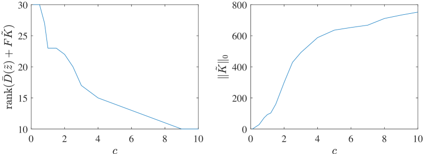
Figure 2: Effect of $c$ with $\varepsilon\equiv 0.1$ for problem $\tilde{\mathbb{P}}_{0}$

Table 3: Method of Section 5 for problem $\tilde{\mathbb{P}}_{2}$

$\rho$	$21$	$16$	$9$	$7$	$5$	$3$
${\rm rank}(\bar{D}(\tilde{z})+F\tilde{K})$	$20$	$15$	$8$	$6$	$4$	$2$
$\|[\bar{H},\Pi]\tilde{K}\|_{2}$	$0$	$0.48$	$1.15$	$1.23$	$1.40$	$1.58$

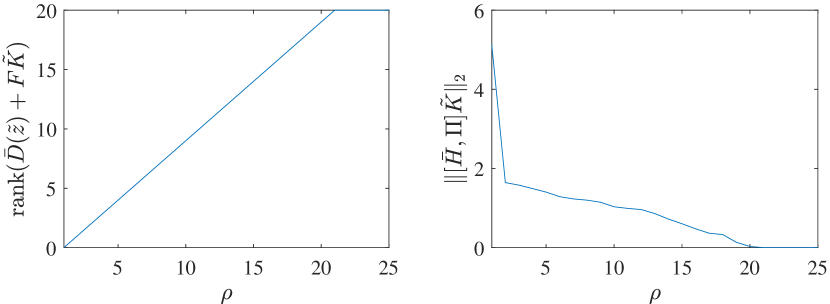
Figure 3: Method of Section 5 for problem $\tilde{\mathbb{P}}_{2}$

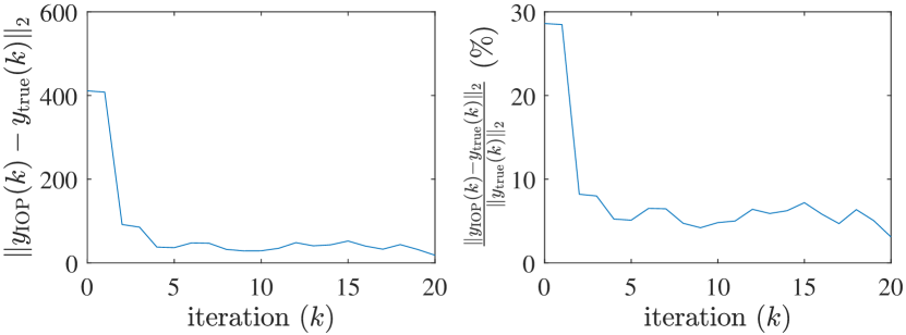
Figure 4: Data disutility of problem $\tilde{\mathbb{P}}_{2}$

Problem $\tilde{\mathbb{P}}_{2}$. In this case, $\bar{G}$ and $\bar{H}^{e}$ are randomly generated such that Assumption 5.1 holds. We then apply Algorithm 1. In the simulation, we have $n=10$, $q^{e}=10$, ${\rm rank}(F)=20$ and ${\rm Tr}(\bar{A})=10$. Hence, we have $\tilde{z}={{\rm Tr}(\bar{A})}/{n}=1$. Table 3 and Fig. 3 show that ${\rm rank}(\bar{D}(\tilde{z})+F\tilde{K})=\rho-1<\rho$ for each $\rho$. This verifies that the construction of $K$ given by Lemma 5.1 is feasible for problem (5.1). Table 3 and Fig. 3 also show that the smaller the value of $\rho$, the larger the value of $\|[\bar{H},\Pi]\tilde{K}\|_{2}$. Given a perturbed system derived under a specific $\rho$, we use the mechanism introduced at the second last paragraph of Section 3.2 to check which data items can be inferred and which cannot. When $\rho=21$, $(T_{10}(0),V_{3},V_{8})$ can be inferred; when $\rho=19$, only $V_{8}$ can be inferred; when $\rho\leq 18$, for any $i\in\{1,2,\cdots,10\}$, no entry can be inferred. We then design a state feedback controller $u^{c}$ such that each $x_{i}$ is stabilized at 21.5 degrees. In the control problem, each $V_{i}$ is viewed as an external noise and is generated as a random integer between 0 to 10 at each iteration. The data disutility of problem $\tilde{\mathbb{P}}_{2}$ is shown in Fig. 4, in which $y_{\rm true}$ is the unperturbed output and $y_{\rm IOP}$ is the perturbed output (IOP indicates input-output perturbations). We can see that the data disutility $\|y_{\rm IOP}(k)-y_{\rm true}(k)\|_{2}$ is below 10% of $\|y_{\rm true}(k)\|_{2}$ after 5 iterations.

We also simulate the differentially private scheme in the paper (Le Ny and Pappas, 2014) with $\varepsilon=0.1$ (i.e., $0.1$-differential privacy) on the HVAC problem. Fig. 5 shows the comparison with our algorithm for problem $\tilde{\mathbb{P}}_{2}$ in terms of data utility. In Fig. 5, $y_{\rm true}$ and $y_{\rm IOP}$ have the same meanings as those in Fig. 4, and $y_{\rm DP}$ is the perturbed output by (Le Ny and Pappas, 2014)’s scheme (DP indicates differential privacy). The first row shows data disutility of our method and the second row shows that of the paper (Le Ny and Pappas, 2014). From Fig. 5, we can see that our method achieves much better data utility than the differential privacy method of the paper (Le Ny and Pappas, 2014) when $\varepsilon=0.1$.

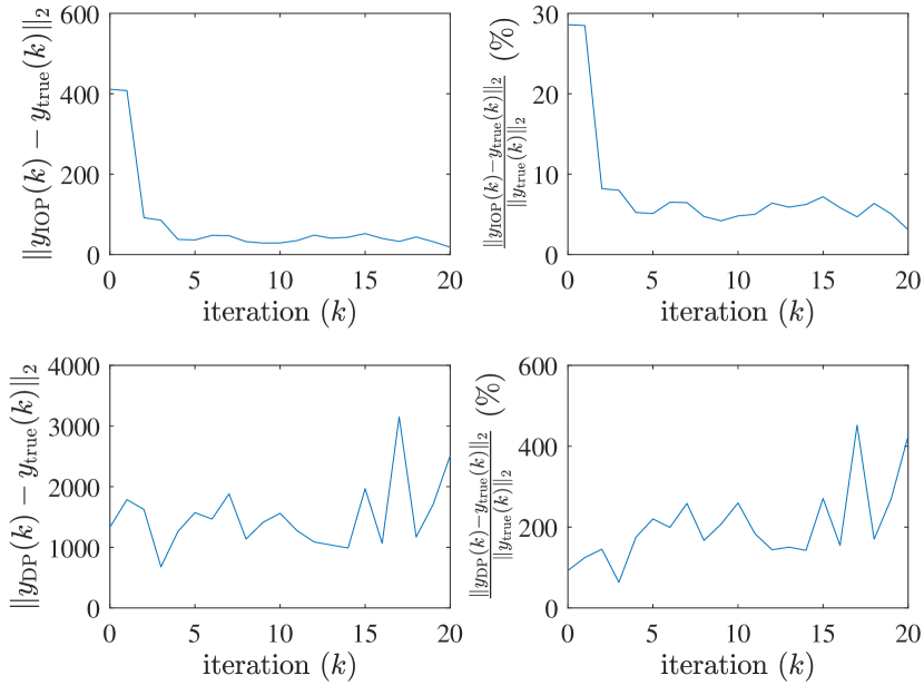
Figure 5: Comparison with differential privacy for problem $\tilde{\mathbb{P}}_{2}$

We also simulate the SDP approach (23) with the last constraint dropped. The average time of solving the SDP of (23) once is 8.18 seconds, while the average time of running Algorithm 1 once is 0.0048 seconds. As mentioned in the paragraph right below (23), one only needs to tune $\rho$ for at most $\min\{n+q,n+p\}$ times. For this example, $\min\{n+q,n+p\}=20$. Hence, for the worst case, one needs to run Algorithm 1 twenty times and the total running time is approximately $0.0048\times 20=0.096$ seconds, which is still much shorter than solving the SDP of (23) once. This verifies that Algorithm 1 is computationally more efficient than the SDP approach.

7 Conclusions

This paper formulates the problem of perturbation design to achieve privacy-preserving data release of linear dynamic networks. The computational complexity of the formulated optimization problem is analyzed. An SDP relaxation for the $\ell_{0}$ minimization is derived. For a class of $\ell_{2}$ minimizations, we provide a computationally more efficient method which can return an analytic feasible solution. A case study on an HVAC system is conducted to validate the efficacy of the developed techniques.

8 Appendix

In this section, we first provide an introduction to $\ell$-diversity. After that, we illustrate how to extend $\ell$-diversity to construct Definition 2.1 in our problem setting.

Table 4: A 3-diverse salary/disease table

ZIP code	Age	Salary	Disease
476**	2*	3K	gastric ulcer
476**	2*	4K	gastritis
476**	2*	5K	stomach cancer
4790*	$\geq 40$	6K	gastritis
4790*	$\geq 40$	11K	flu
4790*	$\geq 40$	8K	brochitis
476**	3*	7K	bronchitis
476**	3*	9K	pneumonia
476**	3*	10K	stomach cancer

Informally speaking, the notion of $\ell$-diversity requires that, given the adversary’s observations, there is adequate diversity in each sensitive attribute of the dataset in the released table. The work Li et al. (2007) formally defines $\ell$-diversity as that each equivalence class of the released table has at least $\ell$ “well-represented” values for each sensitive attribute. An equivalence class of an anonymized table is a set of records that share the values of the attributes the adversary may know. Having $\ell$ “well-represented” values essentially means that the probabilities of these $\ell$ values are close to each other and meanwhile the total probability of these $\ell$ values is significant, e.g., equal or close to 1. We adopt the following example from Li et al. (2007) to illustrate the notion of $\ell$-diversity. Table 4 is an anonymized table with four attributes, namely, ZIP code, Age, Salary and Disease, in which the adversary might observe ZIP codes and Ages of some records, while Salary and Disease are sensitive attributes which should not be disclosed to the adversary. Each * represents an anonymized digit. Each equivalence class shares the values of ZIP code and Age. So there are three equivalence classes: rows 1–3, rows 4–6 and rows 7–9. Since each equivalence class has three different values for each of Salary and Disease, Table 4 has 3-diversity. Assume that the adversary knows that a specific participant has ZIP code 47630 and age 33 and aims to infer this participant’s salary and type of disease. Through Table 4, the adversary can tell that this participant’s record belongs to the equivalence class formed by the last three rows. However, since this equivalence class has 3-diversity, the adversary cannot uniquely determine the participant’s salary or type of disease.

Table 5: An illustrative example

$y$	$x_{1}(0)$	$x_{2}(0)$
2	1	1
2	2	0
2	0	2
$\vdots$	$\vdots$	$\vdots$
3	1	2
3	2	1
3	3	0
$\vdots$	$\vdots$	$\vdots$
$\vdots$	$\vdots$	$\vdots$

Table 6: Hypothetical released table

$\{y(k)\}$	$x_{1}^{n}(0)$	$\cdots$	$x_{d_{x}^{n}}^{n}(0)$	$\{u_{1}^{n}(k)\}$	$\cdots$	$\{u_{d_{u}^{n}}^{n}(k)\}$	$x_{1}^{t}(0)$	$\cdots$	$x_{d_{x}^{t}}^{t}(0)$	$\{u_{1}^{t}(k)\}$	$\cdots$	$\{u_{d_{u}^{t}}^{t}(k)\}$
Equivalence class 1
Equivalence class 2
$\vdots$

The notion of diversity can be interpreted as a measure of uncertainty: a larger diversity indicates that the uncertainty on the sensitive attributes is also larger. In our paper, to make an analogy between $\ell$-diversity and our privacy notion Definition 2.1, we can use the output sequence $\{y(k)\}$ as the label of an equivalence class and view each of the adversarial data requester’s target entries (i.e., $x^{t}(0)$ and $u^{t}$) as a sensitive attribute. To fix idea, we first provide an illustrative example. For simplicity, let $\hat{A}$, $\hat{B}$ and $\hat{H}$ all be zero matrices and $\hat{G}=[1,1]$. Then the system becomes the single constant output equation $y=x_{1}(0)+x_{2}(0)$, where $x_{1}(0)$ and $x_{2}(0)$ are sensitive attributes and $y$ is the data requester’s observation. The released table is in the form of Table 5. In Table 5, each real number for $y$ generates an equivalence class and each equivalence class has infinite diversity/uncertainty on both $x_{1}(0)$ and $x_{2}(0)$. Using the observed output $y$, say $y=2$, the data requester can determine that $x_{1}(0)$ and $x_{2}(0)$ must take values in one record of the equivalence class corresponding to $y=2$. Since $x_{1}(0)$ and $x_{2}(0)$ could be any point on the line $x_{1}(0)+x_{2}(0)=2$, the diversity/uncertainty on $x_{1}(0)$ and $x_{2}(0)$ is infinite.

We next illustrate how to construct the released table for the general case of our problem. The following notations are consistent with those used in Section 2.3. Our hypothetical released table has the form of Table 6. In Table 6, each equivalence class is a set of initial states and inputs which produce the same $\{y(k)\}$. To be more specific, each equivalence class labeled by a specific output sequence $y_{[0,\kappa]}$ includes the target entries $(x^{t}(0),u^{t}_{[0,\kappa]})$ of $\Delta_{\hat{A},\hat{B},\hat{G},\hat{H}}(y_{[0,\kappa]})$, together with admissible non-target entries $(x^{n}(0),u^{n}_{[0,\kappa]})$. Similar to $\ell$-diversity, our privacy goal is to guarantee that each equivalence class has adequate diversity/uncertainty on each of the target entries $(x_{1}^{t}(0),\cdots,x_{d_{x}^{t}}^{t}(0),u_{1}^{t},\cdots,u_{d_{u}^{t}}^{t})$. In $\ell$-diversity, sensitive attributes take discrete values and the diversity on each sensitive attribute is defined by the number of different valuations for that attribute in each equivalence class. In contrast, the target entries $x^{t}(0)$ and $u^{t}$ in our paper are continuous-valued and thus cannot be enumerated (i.e., uncountable). Hence, we need to introduce a new measure to quantify the diversity/uncertainty. In this paper, we propose to measure the diversity/uncertainty by the diameter of the set $\Delta_{\hat{A},\hat{B},\hat{G},\hat{H}}(y_{[0,\kappa]})$. For each target entry, a larger diameter indicates a larger range of admissible valuations and thus a larger diversity/uncertainty. An infinite diameter achieves the largest possible diversity/uncertainty. Hence, for our problem setting, we say that privacy is preserved if the diameter of the set $\Delta_{\hat{A},\hat{B},\hat{G},\hat{H}}(y_{[0,\kappa]})$ is infinite for any feasible output sequence $y_{[0,\kappa]}$ for any $\kappa\in\mathbb{N}$. Please refer to Section 2.3 for the detailed definitions and discussions.

References

- Boyd and Vandenberghe (2004) Boyd, S. and Vandenberghe, L. (2004). Convex Optimization. Cambridge University Press.
- Brodkin (2018) Brodkin, J. (2018). Find out if your password has been pwned–without sending it to a server. Technical report, ars Technica.
- California Public Utilities Commission (2010) California Public Utilities Commission (2010). CA senate bill 1476. Technical report.
- Campbell and Meyer (2009) Campbell, S.L. and Meyer, C.D. (2009). Generalized Inverses of Linear Transformations. Society for Industrial and Applied Mathematics (SIAM).
- Candes and Tao (2005) Candes, E. and Tao, T. (2005). Decoding by linear programming. IEEE Transactions on Information Theory, 52(12), 4203–4215.
- Cavoukian (2012) Cavoukian, A. (2012). Smart meters in Europe: Privacy by design at its best. Technical report, Information and Privacy Commissioner, Ontario, Canada.
- Chen (1999) Chen, C.T. (1999). Linear System Theory and Design. Oxford University Press.
- Coleman and Pothen (1986) Coleman, T. and Pothen, A. (1986). The null space problem. I. complexity. SIAM J. Algebraic Discrete Methods, 7(4), 527–537.
- Donoho (2006) Donoho, D. (2006). Compressed sensing. IEEE Transactions on Information Theory, 52(4), 1289–1306.
- Dwork and Roth (2014) Dwork, C. and Roth, A. (2014). The algorithmic foundations of differential privacy. Foundations and Trends in Theoretical Computer Science, 9(3–4), 211–407.
- Emami-Naeini and Van Dooren (1982) Emami-Naeini, A. and Van Dooren, P. (1982). Computation of zeros of linear multivariable systems. Automatica, 18(4), 415–430.
- Farebrother (1988) Farebrother, R.W. (1988). Linear Least Squares Computations. CRC Press.
- Fazel et al. (2004) Fazel, M., Hindi, H., and Boyd, S. (2004). Rank minimization and applications in system theory. In American Control Conference, 3273–3278.
- Goldwasser and Micali (1984) Goldwasser, S. and Micali, S. (1984). Probabilistic encryption. Journal of Computer and System Sciences, 28(2), 270–299.
- Han et al. (2016) Han, S., Topcu, U., and Pappas, G.J. (2016). Event-based information-theoretic privacy: A case study of smart meters. In American Control Conference, 2074–2079.
- Hautus (1983) Hautus, M.L.J. (1983). Strong detectability and observers. Linear Algebra and its Applications, 50, 355–368.
- Hopping (2017) Hopping, C. (2017). Google brings data loss prevention to its cloud. Technical report, CloudPro.
- Horn and Johnson (1985) Horn, R.A. and Johnson, C.R. (1985). Matrix Analysis. Cambridge University Press.
- Huang et al. (2012) Huang, Z., Mitra, S., and Dullerud, G. (2012). Differentially private iterative synchronous consensus. In ACM workshop on privacy in the electronic society, 81–90.
- Ipsen (2009) Ipsen, I.C.F. (2009). Numerical Matrix Analysis: Linear Systems and Least Squares. Society for Industrial and Applied Mathematics (SIAM).
- Ji et al. (2018) Ji, Y., Wu, Y.C., and Lafortune, S. (2018). Enforcement of opacity by public and private insertion functions. Automatica, 93(7), 369–378.
- Kang et al. (2014) Kang, C., Park, J., Park, M., and Baek, J. (2014). Novel modeling and control strategies for a HVAC system including carbon dioxide control. Energies, 7(6), 3599–3617.
- Kelman and Borrelli (2011) Kelman, A. and Borrelli, F. (2011). Bilinear model predictive control of a HVAC system using sequential quadratic programming. In IFAC World Congress, 9869–9874.
- Kratz (1995) Kratz, W. (1995). Characterization of strong observability and construction of an observer. Linear Algebra and its Applications, 221, 31–40.
- Kumar and Karthikeyan (2012) Kumar, P.M.V. and Karthikeyan, M. (2012). -diversity on k-anonymity with external database for improving privacy preserving data publishing. International Journal of Computer Applications, 54(14), 7–13.
- Last et al. (2014) Last, M., Tassa, T., Zhmudyak, A., and Shmueli, E. (2014). Improving accuracy of classification models induced from anonymized datasets. Information Sciences, 256(1), 138–161.
- Le Ny and Pappas (2014) Le Ny, J. and Pappas, G.J. (2014). Differentially private filtering. IEEE Transactions on Automatic Control, 59(2), 341–354.
- Leeuwen (1990) Leeuwen, J.V. (1990). Handbook of Theoretical Computer Science. MIT Press.
- Li and Das (2013) Li, N. and Das, S.K. (2013). Applications of -anonymity and -diversity in publishing online social networks. Security and Privacy in Social Networks. Springer.
- Li et al. (2007) Li, N., Li, T., and Venkatasubramanian, S. (2007). t-closeness: Privacy beyond k-anonymity and -diversity. In International Conference on Data Engineering, 106–115.
- Li and Li (2009) Li, T. and Li, N. (2009). On the tradeoff between privacy and utility in data publishing. In ACM SIGKDD International Conference on Knowledge Discovery and Data Mining, 517–526.
- Lindell and Pinkas (2009) Lindell, Y. and Pinkas, B. (2009). Secure multiparty computation for privacy-preserving data mining. Journal of Privacy and Confidentiality, 1(1), 59–98.
- Lisovich et al. (2010) Lisovich, M., Mulligan, D., and Wicker, S. (2010). Inferring personal information from demand-response systems. IEEE Security & Privacy, 8(1), 11–20.
- Lu and Zhu (2015) Lu, Y. and Zhu, M. (2015). Game-theoretic distributed control with information-theoretic security guarantees. IFAC Workshop on Distributed Estimation and Control in Networked Systems, 48(22), 264–269.
- Lu and Zhu (2018) Lu, Y. and Zhu, M. (2018). Privacy preserving distributed optimization using homomorphic encryption. Automatica, 96(10), 314–325.
- Ma et al. (2011) Ma, Y., Anderson, G., and Borrelli, F. (2011). A distributed predictive control approach to building temperature regulation. In American Control Conference, 2089–2094.
- Machanavajjhala et al. (2007) Machanavajjhala, A., Kifer, D., Gehrke, J., and Venkitasubramaniam, M. (2007). -diversity: Privacy beyond k-anonymity. ACM Transactions on Knowledge Discovery from Data, 1(1), 1–52.
- Malle et al. (2017) Malle, B., Kieseberg, P., and Holzinger, A. (2017). Interactive anonymization for privacy aware machine learning. In ECML PKDD 2017 Workshop and Tutorial on Interactive Adaptive Learning, 15–26.
- Maruta and Takarada (2014) Maruta, I. and Takarada, Y. (2014). Modeling of dynamics in demand response for real-time pricing. In IEEE International Conference on Smart Grid Communications, 806–811.
- McLaughlin et al. (2011) McLaughlin, S., McDaniel, P., and Aiello, W. (2011). Protecting consumer privacy from electric load monitoring. In ACM Conference on Computer and Communications Security, 87–98.
- Mo and Murray (2017) Mo, Y. and Murray, R.M. (2017). Privacy preserving average consensus. IEEE Transactions on Automatic Control, 62(2), 753–765.
- Nozari et al. (2016) Nozari, E., Tallapragada, P., and Cortes, J. (2016). Differentially private distributed convex optimization via objective perturbation. In American Control Conference, 2061–2066.
- Pequito et al. (2014) Pequito, S., Kar, S., Sundaram, S., and Aguiar, A.P. (2014). Design of communication networks for distributed computation with privacy guarantees. In IEEE Conference on Decision and Control, 1370–1376.
- Ramasubramanian et al. (2016) Ramasubramanian, B., Cleaveland, R., and Marcus, S.I. (2016). A framework for opacity in linear systems. In American Control Conference, 6337–6344.
- Recht et al. (2010) Recht, B., Fazel, M., and Parrilo, P.A. (2010). Guaranteed minimum-rank solutions of linear matrix equations via nuclear norm minimization. SIAM J. Algebraic Discrete Methods, 52(3), 471–501.
- Samarati and Sweeney (1998) Samarati, P. and Sweeney, L. (1998). Protecting privacy when disclosing information: -anonymity and its enforcement through generalization and suppression. Technical report, SRI-CSL-98-04, SRI Computer Science Laboratory.
- Sankar et al. (2013) Sankar, L., Rajagopalan, S.R., and Poor, H.V. (2013). Utility-privacy tradeoffs in databases: An information-theoretic approach. IEEE Transactions on Information Forensics and Security, 8(6), 838–852.
- Shannon (1949) Shannon, C.E. (1949). Communication theory of secrecy systems. Bell System Technical Journal, 28(4), 656–715.
- Vandenberghe and Boyd (1996) Vandenberghe, L. and Boyd, S. (1996). Semidefinite programming. SIAM Review, 38(1), 49–95.
- Venkitasubramaniam et al. (2015) Venkitasubramaniam, P., Yao, J., and Pradhan, P. (2015). Information-theoretic security in stochastic control systems. Proceedings of the IEEE, 103(10), 1914–1931.
- Wang and Tague (2014) Wang, X. and Tague, P. (2014). Non-invasive user tracking via passive sensing: Privacy risks of time-series occupancy measurement. In 2014 Workshop on Artificial Intelligent and Security Workshop, 113–124.
- Wu and Lafortune (2014) Wu, Y.C. and Lafortune, S. (2014). Synthesis of insertion functions for enforcement of opacity security properties. Automatica, 50(5), 1336–1348.
- Yang and Zhang (2011) Yang, J. and Zhang, Y. (2011). Alternating direction algorithms for -problems in compressive sensing. SIAM Journal on Scientific Computing, 33(1), 250–278.
- Yong et al. (2016) Yong, S., Zhu, M., and Frazzoli, E. (2016). A unified filter for simultaneous input and state estimation of linear discrete-time stochastic systems. Automatica, 63(1), 321–329.
- Zhang et al. (2016) Zhang, H., Shu, Y., Cheng, P., and Chen, J. (2016). Privacy and performance trade-off in cyber-physical systems. IEEE Network, 30(2), 62–66.
- Zhu and Lu (2015) Zhu, M. and Lu, Y. (2015). On confidentiality preserving monitoring of linear dynamic networks against inference attacks. In American Control Conference, 359–364.