Slave-Boson analysis of the 2D Hubbard model

Abstract

We present a comprehensive study of the 2D one-band Hubbard model applying the spin rotation invariant slave-boson method. We utilize a spiral magnetic mean field and fluctuations around a paramagnetic mean field to determine the magnetic phase diagram and find the two approaches to be in good agreement. Apart from the commensurate phases characterized by ordering wave vectors ${\bm{Q}}=(\pi,\pi)$, $(0,\pi)$, and $(0,0)$ we find incommensurate phases where the ordering wave vectors ${\bm{Q}}=(Q,Q)$, and $(Q,\pi)$ vary continuously with filling, interaction strength or temperature. The mean field quantities magnetization and effective mass are found to change discontinuously at the phase boundaries separating the $(Q,Q)$ and $(Q,\pi)$ phases, indicating a first order transition. The band structure and Fermi surface is shown in selected cases. The dynamic spin and charge susceptibilities as well as the structure factors are calculated and discussed, including the emergence of collective modes of the zero sound and Mott insulator type. The dynamical conductivity is calculated in dependence of doping, interaction strength and temperature. Finally, a temperature-interaction strength phase diagram is established.

I Introduction

Strongly correlated electrons on a lattice has proven to be one of the most interesting and challenging topics of contemporary physics, following the discovery of heavy electron systems and of the high $T_{c}$ superconductors. Such systems show a plethora of interesting properties such as metal-insulator transitions, the emergence of long range order such as magnetic, charge or nematic order, and possible non-Fermi liquid behavior of the quasiparticles, in particular near a quantum phase transition, not to mention the up to now still not fully understood electronic pairing mechanism of the high $T_{c}$ superconductors. Most electronic systems in the metallic phase form a Landau Fermi liquid Landau (1957); Baym and Pethick , a state adiabatically connected to the weakly coupled limit, which at low energies in slowly varying external fields is characterized by a only a few parameters $-$ effective mass and Landau interaction functions. The phenomenological Fermi liquid theory appears to work in extreme strong coupling situations as represented, e.g., by the heavy quasiparticle system found in heavy fermion compounds. These successes of  Fermi  liquid theory not withstanding, a microscopic theory of the renormalizations expressed by the Fermi liquid functions is still largely missing, despite decades of research efforts.

The archetypical model of a correlated Fermi system is given by the Hubbard model Hubbard (1963, 1964) $-$ a one-band model of electrons on a lattice subject to on-site interaction $U$. For large $U$ the model captures the competition between kinetic energy favoring mobility and local interaction forcing localization, giving rise to a Mott metal-insulator transition Mott (1949). In order to treat strong correlations, non-perturbative methods are required. A first successful approach, capable of treating the Mott-Hubbard transition, is the so-called Gutzwiller approximation Gutzwiller (1963); Brinkman and Rice (1970); Vollhardt (1984). Initially formulated as a variational problem for the approximate calculation of the energy expectation value of a correlated wave function, it has later been rederived in a slave-boson mean field approximation Kotliar and Ruckenstein (1986). A further widely used approach starts from the limit of infinite coordination number Metzner and Vollhardt (1989); Georges et al. (1996), the Dynamical Mean Field Theory (DMFT). DMFT successfully captures local correlations, and has been widely applied, with remarkable success. The treatment of longer range correlations such as present with incommensurate magnetic order or superconductivity is more difficult within the DMFT framework. Among the many other methods that have been proposed to deal with strongly correlated systems we like to mention a diagrammatic approximation scheme proposed by Bünemann et al. Bünemann et al. (2012) for evaluating Gutzwiller projected states. The method has been applied, e.g., to study superconductivity within the 2D Hubbard model Kaczmarczyk et al. (2013).

The difficulty in treating models of strongly correlated electrons on the lattice is that the dynamics of an electron depends on the occupation of the site it is residing on, which can either be empty ($|0\rangle$), singly occupied ($\left|\uparrow\right\rangle$, $\left|\downarrow\right\rangle$) or doubly occupied ($|2\rangle$). For the Hubbard model with large repulsive on-site interaction $U$, the doubly occupied states will be pushed far up in energy, and will not contribute to the low energy physics. This leads effectively to a projection of Hilbert space onto a subspace without doubly occupied sites. It turns out to be difficult to effect this projection within conventional many-body theory. A powerful technique for describing the projection in Hilbert space is the method of auxiliary particles Frésard et al. (2012): One assigns an auxiliary field or particle to each of the four states $|0\rangle$, $\left|\uparrow\right\rangle$, $\left|\downarrow\right\rangle$, $|2\rangle$ at a given lattice site (considering one strongly correlated orbital per site). The fermionic nature of the electrons requires that two of the auxiliary particles are fermions, e.g., the ones representing $\left|\uparrow\right\rangle$, $\left|\downarrow\right\rangle$, and the remaining two are bosons. There are various ways of defining auxiliary particles for a given problem. This freedom may be used to choose the one which is best adapted to the physical properties of the system. A more complex representation of electron operators in terms of auxiliary particle operators, incorporating the result of the Gutzwiller approximation Gutzwiller (1963) on the slave-boson mean field level, has been developed by Kotliar and Ruckenstein (KRSB) Kotliar and Ruckenstein (1986). Further extensions to multi-band Hubbard models have been introduced as well Frésard and Kotliar (1997); Lechermann et al. (2007). A generalization of the KRSB method to manifestly spin rotation invariant form Li et al. (1989); Frésard and Wölfle (1992) (SRIKR) has been developed, allowing one to address non-collinear spin configurations and transverse spin fluctuations. In particular, the method has been used to describe antiferromagnetic Lilly et al. (1990), spiral Frésard et al. (1991); Igoshev et al. (2013, 2015); Frésard and Wölfle (1992); Möller et al. (1993), and striped Seibold et al. (1998); Lorenzana and Seibold (2002, 2003); Seibold and Lorenzana (2005); Raczkowski et al. (2006, 2007); Fleck et al. (2001) phases. Furthermore, the competition between spiral and striped phases has been studied Raczkowski, M. et al. (2006). In the limit of large $U>60t$, it has been found that the spiral order continuously evolves toward ferromagnetic order.

In this paper we present a detailed derivation of the SRIKR slave-boson formalism (Sec. II and appendices A-F). In Sec. III we apply it to calculate slave-boson mean field solutions and two-particle response functions for the one-band Hubbard model on a two-dimensional square lattice at zero temperature. The magnetic phase diagram in the interaction-density-plane within the manifold of spiral magnetic states is obtained from the mean field analysis. We discuss the energy spectrum and the mass enhancement of quasiparticles at the Fermi level, as well as the Fermi surfaces. The static spin susceptibility is parametrized in terms of a Landau interaction function. The dynamic spin susceptibility is calculated and parametrized in terms of a Landau damping function. At the phase transition, the spin susceptibility at the ordering wave vector is found to diverge as $\chi({\bm{Q}},0)\propto(n-n_{c})^{-\alpha}$ where $n_{c}$ is the critical doping. We determine the phase boundaries to the paramagnetic phase (i) from the mean field equations and (ii) from the divergence of the paramagnetic spin susceptibility at finite wave vector ${\bm{Q}}$. The two methods provide consistent results, where in the case of second order transitions, method (ii) is more efficient, whereas first order transitions can only be found with method (i). The ordering wave vector ${\bm{Q}}$ is found to vary continuously over large parts of the phase diagram, but suffers occasional jumps signaling first order phase transitions. The charge response function is employed to calculate the dynamical conductivity.

In Sec. IV we present results at finite temperature. We determine the magnetic phase diagram in the temperature $T-$ doping $n$ plane at fixed interaction $U$. We determine the phase boundaries separating the magnetically ordered phases from the paramagnetic phase and also separating different ordered states. A continuous change of the ordering wave vector as the temperature and doping are varied is determined. The static spin susceptibility at fixed $U$ and $n$ is found to diverge at the transition as $\chi({\bm{Q}},0)\propto(T-T_{c})^{-1}$, where $T_{c}$ is the critical temperature.

We compare our results with available benchmark results, in particular a recent study of the two-dimensional Hubbard model using Density Matrix Embedded Theory (DMET) Zheng and Chan (2016), finding remarkably good agreement.

II Model and method

This section defines the Hamiltonian and summarizes the most important aspects of spin rotation invariant slave-boson formalism, while a detailed derivation of the method can be found in the appendices A-F. We investigate the one band Hubbard model in two spatial dimensions (2D),

$$H= -\sum_{i,j,\sigma}t_{i,j}c_{i,\sigma}^{\dagger}c^{\vphantom{\dagger}}_{j,\sigma}-\mu_{0}\sum_{i,\sigma}c_{i,\sigma}^{\dagger}c^{\vphantom{\dagger}}_{i,\sigma}+U\sum_{i}c_{i,\uparrow}^{\dagger}c^{\vphantom{\dagger}}_{i,\uparrow}c^{\dagger}_{i,\downarrow}c_{i,\downarrow}^{\vphantom{\dagger}},$$ (1)

where the operator $c_{i,\sigma}^{\dagger}$ creates a fermion on site $i$ with spin $\sigma=\{\uparrow,\downarrow\}$. We allow hopping terms between nearest neighboring sites denoted by $t$ and next nearest neighboring sites by $t^{\prime}$. Further we employ an on-site Hubbard interaction $U$. All energy scales are given in units of $t$.

II.1 Slave-boson representation

We apply the SRIKR slave-boson representation, where the original fermionic operator $c^{(\dagger)}_{i,\sigma}$ is expressed as a combination of the pseudofermion operator $f_{i,\sigma}$ and bosonic operators $e_{i},d_{i},p_{i,\mu}$ with $\mu\in\{0,1,2,3\}$, labeling empty, doubly and singly occupied states, respectively, as

$$c^{\dagger}_{i,\sigma} \equiv\sum_{\sigma^{\prime}}z^{\dagger}_{i,\sigma\sigma^{\prime}}f^{\dagger}_{i,\sigma^{\prime}},$$ (2)

where

$$\underline{\smash{z}}=(e^{\dagger}\underline{\smash{L}}M\underline{\smash{R}}\ \underline{\smash{p}}+\tilde{}\underline{\smash{p}}^{\dagger}\underline{\smash{L}}M\underline{\smash{R}}d),$$ (3a)

with

$$\underline{\smash{L}} =\left((1-d^{\dagger}d)\underline{\smash{\tau}}_{0}-2\underline{\smash{p}}^{\dagger}\underline{\smash{p}}\right)^{-1/2},$$ (3b)

$$M =\left(1+d^{\dagger}d+e^{\dagger}e+\sum\limits_{\mu}p^{\dagger}_{\mu}p^{\vphantom{\dagger}}_{\mu}\right)^{1/2},$$ (3c)

$$\underline{\smash{R}} =\left((1-e^{\dagger}e)\underline{\smash{\tau}}_{0}-2\tilde{\underline{\smash{p}}}^{\dagger}\tilde{\underline{\smash{p}}}\right)^{-1/2}.$$ (3d)

The underbar denotes $2\times 2$ spin matrices, specifically

$$\underline{\smash{p}}=\frac{1}{2}\sum_{\mu=0}^{3}p^{{\vphantom{\dagger}}}_{\mu}\underline{\smash{\tau}}^{\mu},$$ (4)

where $\underline{\smash{\tau}}^{\mu}$ are the Pauli matrices including the unit matrix $\underline{\smash{\tau}}^{0}$, and $\underline{\smash{\tilde{p}}}$ is the time reversed operator of $\underline{\smash{p}}$. This form ensures spin rotation invariance (compare Appendix A) and the correct non-interacting limit within the mean field approximation (compare Appendix C).

The slave-boson representation is complemented by the local constraints

$$1 =e^{\dagger}_{i}e_{i}^{\vphantom{\dagger}}+d^{\dagger}_{i}d_{i}^{\vphantom{\dagger}}+\sum_{\mu=0}^{3}p^{\dagger}_{i,\mu}p^{\vphantom{\dagger}}_{i,\mu}\ ,$$ (5a)

$$\sum_{\sigma}f^{\dagger}_{i,\sigma}f^{\vphantom{\dagger}}_{i,\sigma} =\sum_{\mu=0}^{3}p^{\dagger}_{\mu,i}p^{\vphantom{\dagger}}_{\mu,i}+2d^{\dagger}_{i}d^{\vphantom{\dagger}}_{i}\ ,$$ (5b)

$$\sum_{\sigma\sigma^{\prime}}^{\vphantom{3}}{\bm{\tau}}_{\sigma\sigma^{\prime}}f^{\dagger}_{i,\sigma^{\prime}}f^{\vphantom{\dagger}}_{i,\sigma} =p^{\dagger}_{0,i}{\bm{p}}_{i}^{\vphantom{\dagger}}+{\bm{p}}_{i}^{\dagger}p_{0,i}^{\vphantom{\dagger}}-\mathrm{i}{\bm{p}}_{i}^{\dagger}\times{\bm{p}}_{i}^{\vphantom{\dagger}}\;,$$ (5c)

where ${\bm{\tau}}$ is the three-vector of Pauli matrices. These constraints project onto the physical subspace and are enforced on each lattice site $i$, using the Lagrange multipliers $\alpha_{i}$, $\beta_{0,i}$ and ${\bm{\beta}}_{i}$ within the path integral formulation (compare Appendix B). In Appendix B.4 we show that the SRIKR slave-boson representation exactly recovers the atomic limit by integrating out all fields.

II.2 Mean field approximation

In the slave-boson representation, the interaction term of the Hamiltonian becomes quadratic, at the cost of a non quadratic hopping contribution in bosonic operators. Therefore we employ a (para-) magnetic mean field. In this approximation, the space and time dependent slave-boson fields are replaced by their static expectation value $\psi\rightarrow\langle\psi\rangle$ with $\partial_{\tau}\langle\psi\rangle=0$. A suitable mean field ansatz incorporating a spin spiral with ordering vector ${\bm{q}}$ is given by Möller and Wölfle (1993),

$$\begin{split}e_{i}&\rightarrow\langle e\rangle\in\mathbbm{R}_{0}^{+},\\ p_{0,i}&\rightarrow\langle p_{0}\rangle\in\mathbbm{R}_{0}^{+},\\ d_{i}&\rightarrow\langle d\rangle\in\mathbbm{R}_{0}^{+},\ \partial_{\tau}\langle d\rangle=0,\\ i\beta_{0,i}&\rightarrow\langle\beta_{0}\rangle\in\mathbbm{R},\\ i\alpha_{i}&\rightarrow\langle\alpha\rangle\in\mathbbm{R},\\ {\bm{p}}_{i}&\rightarrow\langle p\rangle\begin{pmatrix}\cos(\phi_{i})\\ \sin(\phi_{i})\\ 0\end{pmatrix},\ \langle p\rangle\in\mathbbm{R}_{0}^{+},\\ i\beta_{i}&\rightarrow\langle\beta\rangle\begin{pmatrix}\cos(\phi_{i})\\ \sin(\phi_{i})\\ 0\end{pmatrix},\ \langle\beta\rangle\in\mathbbm{R},\\ \phi_{i}&\equiv{\bm{q}}{\bm{r}}_{i}.\end{split}$$ (6)

To keep the notation short we drop the brackets $\langle\rangle$ in the following. Within this mean field ansatz the Lagrangian is given by

$$\begin{gathered}\mathcal{L}_{{\bm{q}}}=\sum_{\bm{k}}{\bm{f}}^{\dagger}_{\bm{k}}\left(\underline{\smash{H}}_{\bm{k}}[{\bm{q}},\psi]+\partial_{\tau}\right){\bm{f}}^{\vphantom{\dagger}}_{\bm{k}}+N\big{[}Ud^{2}-2\beta p_{0}p\\ -\beta_{0}(p_{0}^{2}+p^{2}+2d^{2})+\alpha(e^{2}+p_{0}^{2}+d^{2}-1+p^{2})\big{]},\end{gathered}$$ (7a)

with

$${\bm{f}}_{\bm{k}}=\begin{pmatrix}f_{\uparrow,{\bm{k}}}\\ f_{\downarrow,{\bm{k}}-{\bm{q}}}\end{pmatrix},$$ (7b)

where $\underline{\smash{H}}_{\bm{k}}[{\bm{q}},\psi]$ is the non interacting Hamiltonian of the pseudo fermions in dependence of the slave-boson mean fields $\psi$ and $N$ is the total number of lattice sites. Due to the form of the constraints, the Free energy per lattice site $F_{\bm{q}}/N$ only depends on two independent bosonic fields, which we choose to be $p_{0}$, $p$ without loss of generality, and the two Lagrange multiplier fields $\beta$ and $\mu_{\text{eff}}=\mu_{0}-\beta_{0}$. After integrating out the pseudofermionic degrees of freedom, it is given by (compare Appendix F)

$$\begin{gathered}\frac{F_{\bm{q}}}{N}=-\frac{T}{N}\sum_{{\bm{k}},\pm}\ln\left[1+e^{-\epsilon_{{\bm{k}},\pm}/T}\right]\\ -\frac{U}{2}(p_{0}^{2}+p^{2}-n)+\mu_{\text{eff}}n-2\beta p_{0}p,\end{gathered}$$ (8)

where $\epsilon_{{\bm{k}},\pm}$ are the eigenvalues of the matrix $\underline{\smash{H}}_{\bm{k}}[{\bm{q}},\psi]$, $n$ is the electron filling per lattice site and $T$ is the temperature.
The saddle point solution for the ground state is determined by minimizing the free energy with respect to $p_{0}$, $p$ and ordering vector ${\bm{q}}$ while maximizing with respect to $\beta$ and $\mu_{\text{eff}}$. The according mean field values of the bosonic fields are denoted by $\bar{\psi}$ and can be characterized by $\bar{p}=0$ describing a paramagnet (PM) and $\bar{p}\neq 0$ yielding magnetic order.

II.3 Fluctuations around the paramagnetic saddle point

In order to calculate response functions, we consider Gaussian fluctuations around the paramagnetic saddle point  Li et al. (1991); Zimmermann et al. (1997), i.e., we expand the action to the second order in bosonic fields $\psi_{\mu}$ around the mean field solution

$$\delta\mathcal{S}^{(2)}=\sum_{q,n}\delta\psi_{\mu}(-{\bm{q}},-i\omega_{n})\mathcal{M}_{\mu\nu}(q)\delta\psi_{\nu}({\bm{q}},i\omega_{n}),$$ (9a)

with the fluctuation matrix

$$\mathcal{M}_{\mu\nu}({\bm{q}},\omega_{n})\equiv\frac{\delta^{2}\mathcal{S}(\psi)}{\delta\psi_{\mu}(-{\bm{q}},-i\omega_{n})\delta\psi_{\nu}({\bm{q}},i\omega_{n})}\ ,$$ (9b)

where $q=({\bm{q}},\omega_{n})^{T}$ and $\omega_{n}=2\pi Tn$ ($n\in\mathbbm{Z}$) is a bosonic Matsubara frequency. The phases of the $e,p_{0}$ and ${\bm{p}}$ fields can be removed by a gauge transformation (compare Appendix B.2), such that only the $d$-field remains complex valued in position space $d\equiv d_{1}+id_{2}$.

Since the fluctuations are calculated by means of functional derivatives, they violate the constraints which are exactly enforced only at the saddle point. Such violations are actually necessary in order to resolve correlations and evaluate whether the system will relax back to the paramagnetic mean field solution or whether it features an instability. Since the Lagrange multipliers are part of the effective field theory, one needs to consider the fluctuation of $\beta_{0}$ and ${\bm{\beta}}$ as well. However, fluctuations in $\alpha$ would yield bosonic occupations per lattice site unequal to one, which can be associated with a violation of the Pauli principle. This needs to be avoided by replacing an arbitrary slave-boson field (we choose $p_{0}$ w.l.o.g) via Eq. (5a), i.e. fluctuating on the subspace where the $\alpha$ constraint is exactly fulfilled (compare Appendix D). We apply the following convention for the ten bosonic fields: $\psi_{1}=e$, $\psi_{2}=d_{1}$, $\psi_{3}=d_{2}$, $\psi_{4}=\beta_{0}$, $\psi_{5,6,7}=p_{1,2,3}$ and $\psi_{8,9,10}=\beta_{1,2,3}$.

Dynamical response functions can be calculated using the path integral (compare Appendix E)

$$\begin{split}\langle\delta\psi_{\mu}^{*}(q)\delta\psi^{\vphantom{\dagger}}_{\nu}(q)\rangle&=\frac{1}{Z^{(2)}}\int D[\psi^{*},\psi]\delta\psi^{*}_{\mu}(q)\delta\psi^{\vphantom{\dagger}}_{\nu}(q)e^{-\delta\mathcal{S}^{(2)}}\\ &=\mathcal{M}^{-1}_{\mu\nu}(q)\\ \text{with}\quad Z^{(2)}&=\int D[\psi^{*},\psi]e^{-\delta\mathcal{S}^{(2)}}.\end{split}$$ (10)

To evaluate these quantities, we apply a Wick rotation $i\omega_{n}\rightarrow\omega+i\eta$, where $\eta\rightarrow 0^{+}$ regularizes diverging terms and needs to be kept finite for most numerical calculations.

II.3.1 Spin susceptibility

The spin susceptibility is defined by

$$\chi^{\alpha\beta}_{\text{s}}(q)=\langle\delta S^{\alpha}_{-q}\delta S^{\beta}_{q}\rangle.$$ (11a)

where $${\bm{S}}$$ is the spin density, which can be written in terms of slave-bosons (compare Appendix E)

$${\bm{S}}=\check{{\bm{p}}}p_{0}\quad\text{with}\ \check{{\bm{p}}}=(p_{1},-p_{2},p_{3})^{T}.$$ (11b)

In the one band Hubbard model, the fluctuation matrix is block diagonal in ($$\beta_{\alpha},p_{\alpha}) (e,d_{1},d_{2},\beta_{0})$$ and since spin and charge sector are decoupled. Hence, the spin susceptibility takes the simple diagonal form

$$\chi_{\text{s}}^{\alpha\beta}(q)=\bar{p}_{0}^{2}\frac{\mathcal{M}_{10,10}(q)}{\mathcal{M}_{7,7}(q)\mathcal{M}_{10,10}(q)-\mathcal{M}_{7,10}(q)\mathcal{M}_{10,7}(q)}\delta^{\alpha\beta}.$$ (11c)

II.3.2 Bare susceptibility and Charge susceptibility

The bare susceptibility can be determined analogously and is defined by

$$\begin{gathered}\chi_{0}(q)\equiv\frac{1}{Z^{(0)}}\int D[f^{*},f]n_{-q}n_{q}e^{-\mathcal{S}^{(0)}}=-2\mathcal{M}_{4,4}(q)\\ \text{with}\quad Z^{(0)}=\int D[f^{*},f]e^{-\mathcal{S}^{(0)}}\end{gathered}$$ (12a)

where $$n_{q}=\sum_{\bm{k}}f^{*}_{{\bm{k}}+{\bm{q}}}f^{\vphantom{\dagger}}_{\bm{k}} \mathcal{S}^{(0)}$$ is the pseudofermion density and is the mean field action.

The charge susceptibility is defined by

$$\chi_{c}(q)=\langle\delta n_{-q}\delta n_{q}\rangle$$ (12b)

where $n$ is the charge density, which can be written in terms of slave-bosons

$$n=1+d^{2}-e^{2}.$$ (12c)

Hence, we find

$$\chi_{c}(q)=2\bar{d}^{2}_{1}\mathcal{M}^{-1}_{2,2}(q)+2\bar{e}^{2}\mathcal{M}^{-1}_{1,1}(q)-2\bar{d}_{1}\bar{e}\left(\mathcal{M}^{-1}_{1,2}(q)+\mathcal{M}^{-1}_{2,1}(q)\right).$$ (12d)

II.3.3 Structure factors

To describe thermal fluctuations at the frequency $\omega$, we define the structure factor, which is given by the real quantity Auerbach (2012)

$$S_{\alpha}({\bm{q}})=-\int\limits_{-\infty}^{\infty}\frac{d\omega}{\pi}\frac{\mathrm{Im}\ \chi_{\alpha}({\bm{q}},\omega+i\eta)}{1-e^{-\omega/T}},$$ (13)

where $\alpha=s$ is called spin structure factor and $\alpha=c$ charge structure factor.

II.4 Dynamical conductivity

With our results for the charge susceptibility $\chi_{c}$, we can calculate the dynamical conductivity as

$$\sigma(\omega+i\eta)=e^{2}\lim_{{\bm{q}}\rightarrow 0}\frac{-i\omega+\eta}{{\bm{q}}^{2}}\chi_{c}({\bm{q}},\omega+i\eta),$$ (14a)

where we have performed the analytical continuation $$i\omega_{n}\rightarrow\omega+i\eta \eta \tau=1/\eta$$. The convergence parameter can be identified with an inverse scattering time of a Drude conductivity

$$\sigma_{D}(\omega,\tau)=\frac{\sigma_{0}}{1+\omega^{2}\tau^{2}}+i\frac{\sigma_{0}\omega\tau}{1+\omega^{2}\tau^{2}}.$$ (14b)

where $\sigma_{0}\propto\tau$. By data fitting, we can determine the DC-conductivity $\sigma_{0}$ and assign sensible results for $\eta\neq 0$ whereas $\sigma_{0}\rightarrow\infty$ for $\eta\rightarrow 0$.

III Results at zero temperature

This section discusses the slave-boson mean field and fluctuation results applied to the 2D Hubbard model at zero temperature.

III.1 Mean field approximation (MFA)

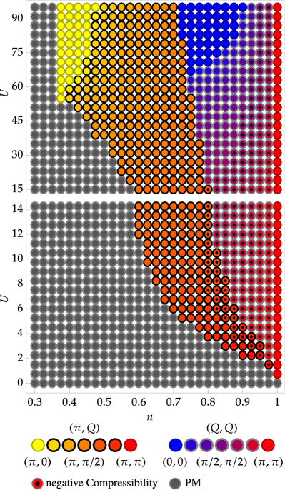
FIG. 1: Magnetic mean field phase diagram for the 2D Hubbard model as function of the interaction $U$ and the filling $n$ without next nearest neighbor hopping ($t^{\prime}=0$) at zero temperature ($T=0$). We only show $n\leq 1$ since the phase diagram for $n>1$ is mirrored due to particle hole symmetry ($n\leftrightarrow 2-n$). It features three distinct phases, namely the PM (gray), a ($\pi,Q$) phase denoted by black circles filled with coloring from red to yellow and a ($Q,Q$) phase denoted by gray circles filled with coloring from red to blue. The ordering vector within one phase regime changes continuously with $U$ and $n$ visualized by the color scheme as indicated in the plot legend. The phase diagram features three commensurate magnetic orderings which are special cases of the above described phases, namely the antiferromagnet (red circle), the ferromagnet (blue circle) and stripe magnetism (yellow circle).

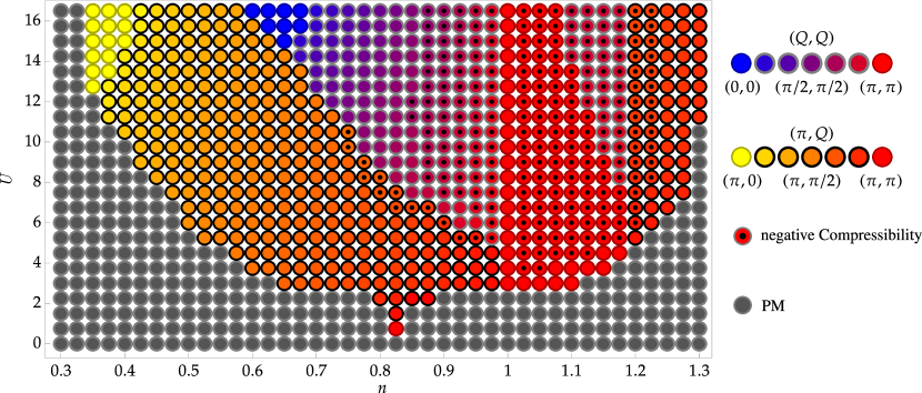
FIG. 2: Magnetic mean field phase diagram for the 2D Hubbard model as function of the interaction $U$ and the filling $n$ with next nearest neighbor hopping ($t^{\prime}=-0.2$) at zero temperature ($T=0$). It features three distinct phases, namely the paramagnet (gray), a ($\pi,Q$) phase denoted by black circles filled with coloring from red to yellow and a ($Q,Q$) phase denoted by gray circles filled with coloring from red to blue. The ordering vector within one phase regime changes continuously with $U$ and $n$ visualized by the color scheme as indicated in the plot legend. The phase diagram features three commensurate magnetic orderings which are special cases of the above described phases, namely the antiferromagnet (red circle), the ferromagnet (blue circle) and stripe magnetism (yellow circle).

We have solved the slave-boson mean field equations presented in subsection II.2 and described in more detail in Appendix F, for the paramagnetic and spiral magnetic phases. We found the minimum of  the resulting free energy, determining the thermodynamically stable phase. In this way we established a phase diagram, presented in the next subsection. An important property of the mean field solution is the renormalization of the fermionic excitation spectrum, given by the factors $z_{0}$ for the paramagnet and $\mathcal{Z}_{+,-}$ for the spiral magnet. Results on the $z-$factors and on several other mean field parameters are presented in the subsequent part. We also show examples of the electronic band structure and the Fermi surface. In addition to magnetic order, charge density wave order may appear. In this work we do not address the case of several types of order being present simultaneously. We do, however, identify signals for the probable appearance of charge order in the presence of magnetic order by studying the compressibility, which is found to turn negative in a certain portion of the magnetically ordered phases.

III.1.1
Magnetic mean field phase diagram

The phase diagram shown in Fig. 1 has been calculated by means of the magnetic mean field theory defined in subsection II.2, putting $t^{\prime}=0$. It complements phase diagrams shown in the literature Frésard and Wölfle (1992); Igoshev et al. (2013) which have only been calculated for smaller $U$. At the phase boundary to the paramagnet, the order parameters $p$ and $\beta$ vanish continuously, i.e., the paramagnetic solution is recovered via a continuous phase transition.
At half filling, the ordering is antiferromagnetic for every finite interaction $U>0$. Away from half filling, within the ordered phase regime, the ordering vector ${\bm{Q}}$ evolves continuously as function of the filling $n$ and interaction $U$. The transitions observed between ($\pi,Q$) and ($Q,Q$) phases are of first order since the order parameter $p$ is found to be discontinuous at the phase boundaries. Furthermore, the phase diagram features three different commensurate magnetic phases, namely the antiferromagnet [${\bm{Q}}=(\pi,\pi)$], ferromagnet [${\bm{Q}}=(0,0)$] and stripe magnetism [${\bm{Q}}=(0,\pi)$]. The ferromagnet features a vanishing double occupancy $d=0$ and $p=p_{0}=\sqrt{n/2}$ which yields the maximum possible magnetization per lattice site $m=pp_{0}=n/2$ (in units of the Bohr magneton) for a given filling. The contribution of fluctuations is expected to lead to $d\neq 0$ and to $m<n/2$ . Every non-ferromagnetic state has a finite double occupancy $d\neq 0$ even on the mean field level.

Fig. 2 shows the magnetic phase diagram for $t^{\prime}=-0.2$, in the extended density regime $0.3<n<1.3$ and is in very good agreement with a previous Slave-boson study Igoshev et al. (2013). At half filling, the tendency towards the antiferromagnet is reduced, because finite $t^{\prime}$ prevents the perfect nesting of the Fermi surface, yielding a paramagnetic regime at weak interaction. On the other hand, at $U\gtrsim 2$, the tendency towards magnetic order is generally increased for larger $|n-1|$, due to the increased hopping range. The next nearest neighbor hopping $t^{\prime}=-0.2$ moves the van Hove singularity, giving rise to an enhanced tendency for magnetic order at $n\approx 0.825$.

III.1.2 Fermionic $z-$factors

The factor $z_{0}$ renormalizes the fermionic band structure in the paramagnetic phase as

$$\epsilon_{{\bm{k}}}=z_{0}^{2}\xi_{{\bm{k}}}-\mu_{\text{eff}}$$ (15a)

where for nearest neighbor hopping $$\xi_{{\bm{k}}}=-2\left[\cos(k_{1})+\cos(k_{2})\right] z_{0} W=8z_{0}^{2} m^{\ast}(k_{1F})=[2z_{0}^{2}\cos(k_{1F})]^{-1}=[2z_{0}^{2}+\mu_{\text{eff}}]^{-1} k_{1F}$$. The factor governs the bandwidth and the effective mass at the Fermi level, e.g. along the x-axis , where is the Fermi wavenumber.

In the magnetically ordered phase the fermionic dispersion is given by

$$\epsilon_{{\bm{k}},\pm}=\frac{1}{4}\left[\zeta_{+}\xi_{{\bm{k}},+}\pm\sqrt{(\zeta_{+}^{2}-\zeta_{-}^{2})\xi_{{\bm{k}},-}^{2}+(\zeta_{-}\xi_{{\bm{k}},+}+4\beta)^{2}}\right]-\mu_{\text{eff}}$$ (15b)

where $\zeta_{\pm}=z_{+}^{2}\pm z_{-}^{2}$, and $\xi_{{\bm{k}},\pm}=\xi_{{\bm{k}}}\pm\xi_{{\bm{k}}+{\bm{Q}}}.$

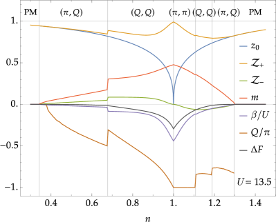
FIG. 3: Magnetic mean field parameters $z_{0}$, $\mathcal{Z}_{\pm}=(z_{+}\pm z_{-})/2$, magnetization $m=pp_{0}$, $\ \beta/U$, ordering vector component $Q$ and the relative difference between the corresponding magnetic and non-magnetic free energy $\Delta F$, versus filling $n$ at $U=13.5$ and at $t^{\prime}=-0.2$. The vertical grid lines indicate a phase transition and the respective phases are denoted in the upper part of the plot.

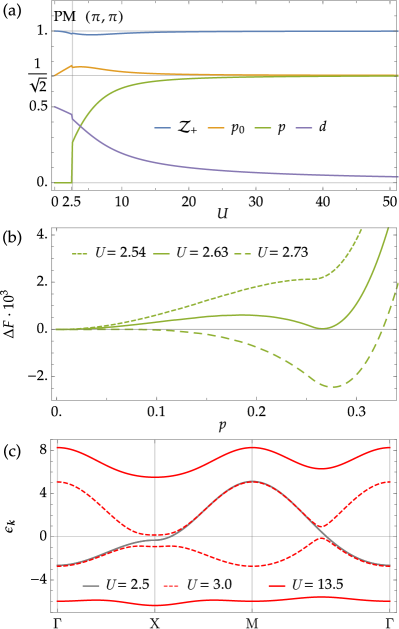
FIG. 4: (a) Magnetic mean field parameters $\mathcal{Z}_{+},p_{0},p,d$ at half filling $n=1$ versus $U$ at $t^{\prime}=-0.2$. The vertical grid lines indicate phase transitions and the respective phases are denoted in the upper part of the plot. (b) Free energy as a function of order parameter $p$ at $n=1$ for various $U$ at $t^{\prime}=-0.2$. The coexistence of two different minima of equal energy at $U=2.63$ indicates a phase transition of first order. (c) Band structure at $n=1$ for various $U$ at $t^{\prime}=-0.2$ on the high symmetry path $\Gamma$–X–M–$\Gamma$ of the non-magnetic Brillouin zone. We show only one spin degenerate band for the paramagnetic case (gray), whereas the magnetic spectrum (red) splits due to translation- and spin rotation symmetry breaking.

Fig. 3 shows the quasiparticle renormalization factors $z_{0}$ for the paramagnet and $\mathcal{Z}_{\pm}=(z_{+}\pm z_{-})/2$ for magnetic state as a function of $n$ for fixed $U=13.5$ for $t^{\prime}=-0.2$. Also shown are the quantities $m=pp_{0},\ \beta/U,$ and the condensation energy $\Delta F=F_{\text{mag}}-F_{\text{para}}$ of the magnetic phases. The various ordered phases are indicated and their respective incommensurate wave vector components $Q$ are also shown as functions of density $n$. The interaction is chosen to be greater than the critical value $U_{c}$ separating the metallic and the Mott insulating phase in a hypothetical paramagnetic phase at half-filling (we determine the critical value of $U$ as $U_{c}=128/\pi^{2}\approx 12.97$ for $t^{\prime}=0$ and $U_{c}\approx 13.1$ for $t^{\prime}=-0.2$). Therefore $z_{0}$ is found to vanish for $n\rightarrow 1$, $z_{0}^{2}\propto|n-1|$, causing the effective mass to diverge, $m^{\ast}\propto 1/|n-1|$. By contrast, in the magnetically ordered phase $z_{\pm}$ stays finite, but $z_{+}-z_{-}\rightarrow 0$, as $n\rightarrow 1$. Consequently, the two dispersions take the limiting values $\epsilon_{{\bm{k}},\pm}=\frac{1}{4}\left(\zeta_{+}\xi_{{\bm{k}},+}\pm\sqrt{\zeta_{+}^{2}\xi_{{\bm{k}},-}^{2}+4\beta^{2}}\right)-\mu_{\text{eff}}$ as $n\rightarrow 1$ , indicating a band insulator with excitation gap $2|\beta|$. However, as shown next, in the limit of large $U$ one finds $2|\beta|\rightarrow U$, which is the signature of a Mott insulator.

To supplement the discussion of the energy bands at half-filling, we show in Fig. 4a the parameters $\mathcal{Z}_{+},p_{0},p,d$ as a function of $U$. In the limit of large $U$ these quantities approach the values $Z_{+}\rightarrow 1$, $p_{0}\rightarrow p\rightarrow 1/\sqrt{2}$, $d\rightarrow 0$. At small $U$ the behavior in the neighborhood of the magnetic transition indicates a first order transition at $U\approx 2.63$. This is clearly seen in the behavior of the free energy as a function of the magnetic order parameter $p$ shown in Fig. 4b. Analogously close to half-filling, the transition from the $(\pi,\pi)-$state to the adjacent $(Q,Q)-$state is also first order, since the ordering wave vector is found to jump from $Q=\pi$ to $Q=0.844\pi$ at $n=1.105$ (see Fig. 3).

III.1.3 Electronic band structure

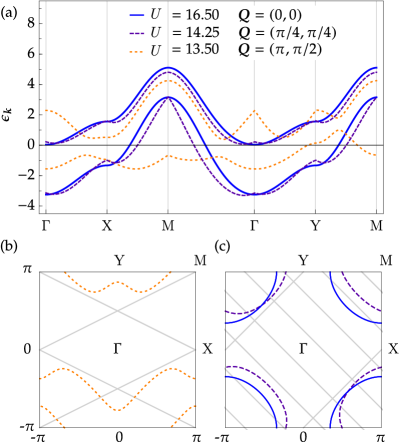
FIG. 5: (a) Band structure at filling $n=0.675$ for the magnetic ordering vectors $(\pi/2,\pi)$ for $U=13.50$, $(\pi/4,\pi/4)$ for $U=14.25$ and $(0,0)$ for $U=16.50$ with $t^{\prime}=-0.2$ on the high symmetry path $\Gamma$–X–M–$\Gamma$–Y–M [X $=(\pi,0)$, Y $=(0,\pi)$, M $=(\pi,\pi)$] of the non magnetic Brillouin zone. Notice, that the ordering vectors $(\pi/2,\pi)$ and $(\pi/4,\pi/4)$ break the $C_{4v}$ symmetry of the non magnetic phase. (b) Fermi surface to the corresponding band structure shown in (a) for $U=13.50$. The gray lines indicate the backfolded Brillouin zone of the magnetic unit cell for the ordering vector $(\pi,\pi/2)$. (c) Fermi surface to the corresponding band structures shown in (a) for $U=14.25$ and $U=16.50$. The gray lines indicate the backfolded Brillouin zone of the magnetic unit cell for the ordering vector $(\pi/4,\pi/4)$.

The dependence of the electronic dispersion on interaction strength and filling is demonstrated in Fig. 4c and Fig. 5. In Fig. 4c we consider the case of half-filling, taking $t^{\prime}=-0.2$. For $U=2.25$, $3.00$, and $13.5$ one observes the splitting of the bands by the onset of magnetic order and the smooth transition of the spectrum as $U$ moves beyond $U=U_{c}$.

To demonstrate the character of the electronic bands in various magnetically ordered phases in Fig. 5a, we fix the density at $n=0.675$, take $t^{\prime}=-0.2$ and plot $\epsilon_{k,\pm}$ along $\Gamma$–X–M–$\Gamma$–Y–M . We choose the interaction such that three different orderings are realized: at $U=13.50$ we have ${\bm{Q}}=(\pi/2,\pi)$, at $U=14.25$ we have ${\bm{Q}}=(\pi/4,\pi/4)$ and at $U=16.50$ the ferromagnetic phase is reached, with ${\bm{Q}}=(0,0)$. The corresponding Fermi surfaces are shown in Fig. 5b ($U=13.5$) and Fig. 5c ($U=14.25$ and $U=16$).

III.1.4 Compressibility

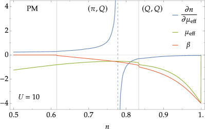
FIG. 6: $\partial n/\partial\mu_{\text{eff}}$, chemical potential $\mu_{\text{eff}}$ and $\beta$ versus filling $n$ at $U=10$ and $t^{\prime}=0$. The compressibility $\kappa_{T}\propto\partial n/\partial\mu_{\text{eff}}$ diverges at the maximum of $\mu_{\text{eff}}$. The vertical gray grid lines indicate phase transitions where the respective phases are denoted in the upper part of the plot and the vertical blue grid line indicates the divergence of the compressibility.

The mean field results allow the calculation of the isothermal compressibility $\kappa_{T}$, or equivalently $\partial n/\partial\mu_{\text{eff}}=n^{2}\kappa_{T}$, as obtained from

$$\frac{\partial n}{\partial\mu_{\text{eff}}}=\frac{\partial(2d^{2}+p_{0}^{2}+p^{2})}{\partial\mu_{\text{eff}}}.$$ (15c)

In Fig. 6, $\partial n/\partial\mu_{\text{eff}}$ is plotted versus $n$ for the nearest neighbor hopping model ($t^{\prime}=0$) and for $U=10.$ Interestingly, the compressibility changes sign in the magnetically ordered phase Frésard and Wölfle (1992); Igoshev et al. (2013) where $\mu_{\text{eff}}$ has a maximum. With increasing density $n$ towards half filling, $|\beta|$ becomes larger and decreases the energy of the occupied band (compare Fig. 3). This has to be counteracted by also reducing $\mu_{\text{eff}}$ to ensure the correct electron filling, causing the compressibility to turn negative. We indicated the portion of the phase diagram where negative compressibility occurs by adding a dot into the colored circles marking the ordering wave vector in Fig. 1 and Fig. 2. A negative compressibility signals a transition to a spatially modulated density distribution or phase separation. The simultaneous presence of two ordering fields, one magnetic, the other nonmagnetic, at generally different ordering vectors, requires a numerical effort beyond the scope of the present work.

III.2 Fluctuations around the paramagnetic mean field

We have calculated the spin and charge susceptibilities in the paramagnetic phase from the fluctuations of the slave-boson fields around the saddle point as described in Appendix D and Appendix E to provide a general stability analysis. The divergence of the static spin (charge) susceptibility at some wave vector indicates the appearance of magnetic (charge) order with a spatial period given by this wave vector. This will be used to determine the magnetic phase boundary of the paramagnet, which turns out to be a numerically more efficient way to identify the appearance of magnetic order, compared to the magnetic mean field analysis presented in the previous subsection. It is reassuring that both methods provide consistent results.

Notice that first order phase transitions cannot be identified via Gaussian fluctuations around a paramagnetic saddle point. This is because a local minimum of the paramagnetic free energy ($p=0$) like, e.g., shown in Fig. 4 is metastable and the global minimum is out of reach of the quadratic expansion of the action.

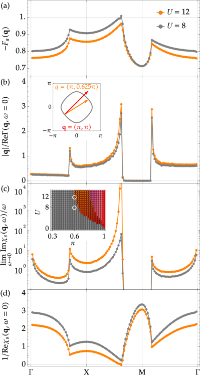
FIG. 7: Spin susceptibility and Landau factors at filling $n=0.6$, $t^{\prime}=0$, $T=0$ and $\eta=0.001$ for $U=8$ (PM) and $U=12$ [phase boundary from PM to $(\pi,Q)$-magnetic order] shown on the high symmetry path $\Gamma$–X–M–$\Gamma$. We show an excerpt of the phase diagram (compare Fig. 1) in the inset of (c), where the two chosen interaction values are highlighted. (a) Landau interaction function $-F_{a}({\bm{q}})$. The phase transition is indicated by $F_{a}({\bm{Q}})=-1$. (b) Landau damping function plotted as $|{\bm{q}}|/\Gamma({\bm{q}},\omega=0)$. Its signal is overall drastically reduced for momenta larger than the diameter of the Fermi surface [compare inset (b)]. (c) Imaginary part of the spin-susceptibility and in the zero frequency limit plotted as $\lim_{\omega\to 0}\operatorname{Im}\chi_{s}({\bm{q}},\omega)/\omega$. Its signal is overall drastically reduced for momenta larger than the diameter of the Fermi surface [compare inset (b)]. (d) Inverse real part of the spin susceptibility. A root of $1/\operatorname{Re}\chi_{s}({\bm{q}},\omega=0)$ indicates a magnetic instability.

III.2.1 Spin susceptibility

Phenomenological form of susceptibility

The functional behavior of the dynamical spin susceptibility at low frequencies can be represented in terms of auxiliary functions $F_{a}({\bm{q}})$ and $\Gamma({\bm{q}},\omega)$. In the static limit we define

$$\chi_{s}({\bm{q}},\omega=0)=\frac{\chi_{0}({\bm{q}},\omega=0)}{1+F_{a}({\bm{q}})}$$ (16a)

where $$F_{a}({\bm{q}}) \chi_{0}({\bm{q}},\omega=0) \Gamma({\bm{q}},\omega)$$ is a generalization of the well-known Landau parameter to finite wave vectors and is the “non-interacting” quasiparticle susceptibility (see Appendix E), which carries a hidden influence of the interaction through its dependence on the mean field parameters. At small but finite frequency the leading dynamical addition is given by the Landau damping term in the denominator, parametrized by a function

$$\chi_{s}({\bm{q}},\omega)=\frac{\chi_{0}({\bm{q}},\omega=0)}{1+F_{a}({\bm{q}})-i\omega/\Gamma({\bm{q}},\omega)}.$$ (16b)

These quantities are shown in Fig. 7a and Fig. 7b at $$n=0.6 t^{\prime}=0 U=8 U=12 \Gamma \Gamma \operatorname{Im}\Gamma=\mathcal{O}(\omega) \omega {\bm{q}}\approx(\pi,\pi) \chi_{s} 1/\Gamma \Gamma |{\bm{q}}|/\Gamma({\bm{q}},\omega=0) |{\bm{q}}|/\Gamma({\bm{q}},\omega=0)\rightarrow const. {\bm{q}}\rightarrow 0 F_{a}({\bm{q}}) \Gamma \Gamma U=12 F_{a}({\bm{q}})=-1 {\bm{Q}}$$, for interactions and on the high symmetry path –X–M– in the Brillouin zone. The corresponding susceptibility will be discussed below. The imaginary part is negligible at small . Around the M point, the wavevector is larger than the diameter of the Fermi surface, as shown in the inset of Fig. 7b and therefore the imaginary part of and consequently of  is zero (compare Fig. 7b). Rather than plotting , we therefore show . The limiting behavior of as is demonstrated. The upper panel shows along –X–M–. The curve for is seen to reach , signaling a phase transition into a magnetically ordered state characterized by the wave vector , which is discussed below.

Magnetic instability

In Fig. 7 the imaginary (c) and real (d) part of the spin susceptibility at $n=0.6$ and $t^{\prime}=0$ are shown for two different interactions. For $U=8$ we find a stable paramagnet for any wavevector and for $U=12$ a magnetic instability appears at the incommensurate ordering vector ${\bm{Q}}\approx(0.625\pi,\pi)$.

A magnetic phase transition is indicated if $\chi_{s}({\bm{q}},\omega=0)$ diverges at some ordering vector ${\bm{q}}={\bm{Q}}$. It is numerically more viable to investigate $1/\operatorname{Re}\chi_{s}({\bm{q}},\omega=0)$, a sign change of $1/\operatorname{Re}\chi_{s}$ indicates a divergence of $\operatorname{Re}\chi_{s}$. This represents the most precise criterion to define a magnetic instability. The imaginary part can be evaluated numerically only at finite $\eta$ and $\omega$, since $\operatorname{Im}\chi_{s}({\bm{q}},\omega+i\eta)\propto\omega$ in the limit $\eta\rightarrow 0$. In Fig. 7c we show $\lim_{\omega\rightarrow 0}[\operatorname{Im}\chi_{s}({\bm{q}},\omega+i\eta)/\omega]$ as a function of ${\bm{q}}$ exhibiting a diverging peak at ${\bm{q}}={\bm{Q}}$, as $U$ increases towards the critical value of $U_{c}\approx 12$. The growth of peaks at other ordering vectors can be explained by the enhancement of the density of states at the Fermi level and do not indicate a magnetic instability.

To determine the paramagnetic phase boundary from the divergence of the static spin susceptibility, we steadily increase the interaction $U$ and look for the first appearance of a zero of $1/\chi_{s}({\bm{Q}},\omega=0)$ as shown in Fig. 7d by example. Following this procedure, the phase boundaries to the paramagnet obtained by the magnetic mean field analysis shown in Fig. 1 and Fig. 2 are reproduced consistently.

Identifying the onset of magnetic instabilities from a study of the spin susceptibility as compared to solving the saddle point equations of the spiral magnetic mean field ansatz is more general. In contrast to the latter, which is restricted to the assumed form of the order (spin spiral), the divergence of the susceptibility signals the emergence of magnetic order of any kind with spatial periodicity described by the wavevector ${\bm{Q}}$. The fluctuation approach is, however, not suited to determine the type of magnetic order beyond the boundary of the paramagnetic regime.

Critical exponent

We determine the critical exponent $\alpha$ at magnetic instabilities of the paramagnet where the spin susceptibility diverges as

$$\chi_{s}({\bm{Q}},0)\propto(n_{c}-n)^{-\alpha},\text{ \ \ }n<n_{c},$$ (17)

when $n\rightarrow n_{c}$. We find a critical exponent of $\alpha=1$ for phase transitions towards the commensurate antiferromagnet ${\bm{Q}}=(\pi,\pi)$ which occupies an extended domain in the phase diagram for $t^{\prime}\neq 0$ as shown in Fig. 2. For incommensurate magnetic instabilities, the critical exponent is found as $\alpha\approx 1/2$, as demonstrated in Fig. 8 for $t^{\prime}=0$ and $U=12$, which shows the inverse spin susceptibility at ${\bm{Q}}\approx(0.625\pi,\pi)$ as function of the filling $n$.

III.2.2 Charge susceptibility

We also considered the possibility of charge order in the Hubbard model as indicated by a divergence of $\chi_{c}({\bm{Q}},0)$ . In the paramagnetic regime, we did not find any charge instabilities for $U\geq 0$, which confirms the magnetic phase diagrams shown in Fig. 1 and Fig. 2. However, we cannot exclude a combination of spin and charge order in the magnetically ordered regime, because the investigation would require fluctuations around a magnetic saddle point, which is outside the scope of our present work. Such an analysis would certainly be of interest, especially in the regime of negative compressibility.

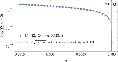
FIG. 8: Inverse static spin susceptibility (blue plot markers) at wave vector $(\pi,0.625\pi)$ versus $n$ at $U=12$ in the paramagnetic regime. The gray dashed line shows a fit of $1/\chi_{s}({\bm{Q}},\omega=0)$ to the square root $\sqrt{n_{c}-n}$, indicating a critical exponent of $\alpha=1/2.$ The vertical line marks the magnetic phase transition at the critical doping $n_{c}$.

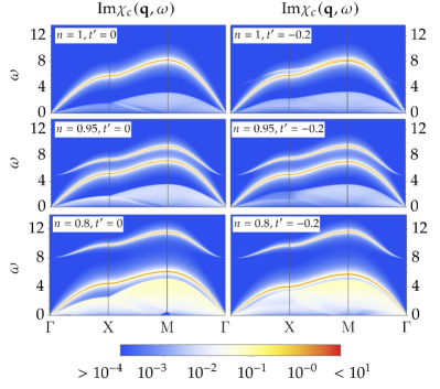
FIG. 9: (a) Imaginary part (color coded) of the bare susceptibility $\chi_{0}$ (left column) and charge susceptibility $\chi_{c}$ (right column) in the frequency $\omega-$wavevector ${\bm{q}}$ plane at $n=0.6$, and $t^{\prime}=0$ for various interaction strengths. For $U>0$, the $\chi_{s}$ features a collective mode and the upper Hubbard band in addition to the particle hole excitation spectrum. (b) Imaginary part of the charge susceptibility $\chi_{c}$ versus frequency $\omega$ at wavevector ${\bm{q}}=(\pi,0)$ at $n=0.6$, $U=10$ and $U=0$ and at $t^{\prime}=0$.

In Fig. 9a we present in the left column the “bare” susceptibility $\chi_{0}$ (corresponding to the bubble diagram in mean field approximation, and therefore dependent on interaction) as function of momentum ${\bm{q}}$ and frequency $\omega$ and compare it with the the charge susceptibility $\chi_{c}$ (right column of Fig. 9a). The chosen set of parameters ($n=0.6,t^{\prime}=0,U=0,2,10$) lies within the paramagnetic regime of the phase diagram Fig. 1. The bare susceptibility is determined by the paramagnetic mean field band structure, given by the spin degenerate eigenvalue $\epsilon_{{\bm{k}}}=-2z_{0}^{2}\left[\cos(k_{1})+\cos(k_{2})\right]-\mu_{\text{eff}}$ (compare Appendix C). The slave-boson renormalization $z_{0}(U)$ depends on the interaction and is normalized to $z_{0}(0)=1$, the resulting bandwidth is given by $W(U)=8z_{0}^{2}(U)$. Hence, for vanishing interaction, we have $W=8$ and accordingly the width of the excitation spectrum is equal to the bandwidth, as can be seen in the top panel of Fig. 9a, moreover it is $\chi_{c}=\chi_{0}$ for $U=0$. Increasing the interaction has two effects. First, the excitation widths of $\chi_{0}$ are reduced, matching the renormalized bandwidths $W(2)\approx 7.8$ and $W(10)\approx 6.5$. Second, $\chi_{c}$ exhibits the emergence of two excitation gaps, splitting the charge susceptibility into three regimes Dao and Frésard (2017). There is a particle-hole excitation continuum for $\omega<W$, where $\chi_{c}$ resembles $\chi_{0}$ and also scales with the bandwidth. The second regime, which may be identified with the upper Hubbard band, features a sharp energy momentum relation and is separated from the first regime by a gap, which approaches $U$ in the limit of large interactions (upper excitation band). This is due to the fact that $\chi_{c}$ as a fluctuation quantity goes beyond the band structure picture of the mean field and allows excitations which result in the creation of new doubly occupied sites at the cost of the interaction $U$. The feature we identify with excitations into the the upper Hubbard band is seen to vanish for ${\bm{q}}\rightarrow 0$ . Third, a collective mode feature situated between the continuum and the upper Hubbard band emerges, which may be identified as a collective density mode as appears in a Fermi liquid for sufficiently large repulsive interaction. At half-filling only one collective mode is visible. This is different for the longer range hopping model ($t^{\prime}=-0.2$) for which both excitation features are present even at half-filling as shown in Fig. 10. The structure of the charge excitation spectrum as a function of frequency at ${\bm{q}}=(\pi,0)$ (X point) is shown in more detail at doping $n=0.6$ , $t^{\prime}=0$ and for $U=10$ and $U=0$ in Fig. 9b. The comparison shows how the interaction (i) shifts spectral weight from the lower to the upper Hubbard band and (ii) generates a collective mode at the upper edge of the lower Hubbard band. The reason for the appearance of two excitation bands lies in the different dynamics of the fermionic and bosonic degrees of freedom. As shown in Appendix E the charge susceptibility is determined by inverse matrix elements of the $4\times 4$ charge block of the fluctuation matrix $\mathcal{M}_{\mu\nu}({\bm{q}},\omega)=\mathcal{M}_{\mu\nu}^{B}({\bm{q}},\omega)+\mathcal{M}_{\mu\nu}^{F}({\bm{q}},\omega)$, $\mu,\nu\in(e,d_{1},d_{2},\beta_{0})$. In opposite to the spin sector, $\mathcal{M}_{\mu\nu}^{B}({\bm{q}},\omega)$ explicitly depends on the frequency because the slave-boson field $d=d_{1}+id_{2}$ is complex valued. Our results are in full agreement with the detailed analysis of collective charge modes in the Hubbard model presented in Dao and Frésard (2017).

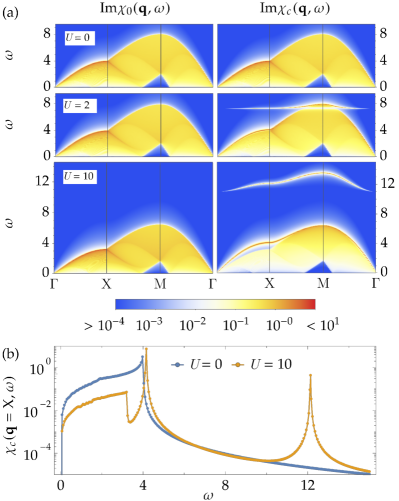
FIG. 10: Imaginary part (color coded) of the charge susceptibility $\chi_{c}$ in the frequency $\omega-$wavevector ${\bm{q}}$ plane for $U=10$ and various dopings $n$ at $t^{\prime}=0$ (left column) and $t^{\prime}=-0.2$ (right column). With increasing $n$ towards half filling, the spectral weight of the particle hole continuum is shifted towards the collective mode. The upper Hubbard band vanishes at half filling for $t^{\prime}=0$ and is kept for the long range hopping model $t^{\prime}=-0.2$.

III.3 Dynamical conductivity

We studied the dynamical conductivity $\sigma(\omega+i\eta)$ according to subsection II.4. In Fig. 11, results for the real (a) and imaginary (b) part of the dynamical conductivity are presented for the nearest neighbor hopping model ($t^{\prime}=0$), at quarter filling $n=0.5$ and for two values of interaction, $U=0$ and $U=35$. The parameter $\eta=1/\tau=0.1$ is kept finite and is identified with the inverse scattering time of the Drude model, which fits our data. For $\eta\rightarrow 0$, the DC-conductivity goes to infinity, because our model does not include a momentum dissipation mechanism (no umklapp scattering, no phonons). One may interpret $\eta$ as an effective scattering parameter accounting for impurity scattering, while the limit $\eta\rightarrow 0$ corresponds to a perfect, impurity-free crystal.

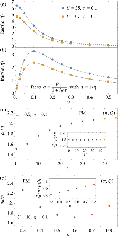
FIG. 11: (a,b) Real and imaginary part of the dynamical conductivity for $\eta=0.1$, $T=0$, quarter filling $n=0.5$ for the two interactions $U=0$ and $U=35$ at $t^{\prime}=0$ . In both cases we see a Drude-like behavior according to Eq. (14b) as indicated by the dashed gray lines. (c) DC-resistivity $\rho_{0}$ versus interaction $U$ for filling $n=0.5$. The inset shows the scaling of $\rho_{0}$ with $1/z_{0}^{2}$. The vertical grid lines indicate phase transitions, the respective phases are denoted in the upper part of the plot and the color of the plot makers display the value of the ordering vector (compare Fig. 1). (d) DC-resistivity $\rho_{0}$ versus doping $n$ for $U=10$. The inset shows the approximate scaling of $\rho_{0}$ with $1/(z_{0}^{2}n)$. The vertical grid lines indicate phase transitions, the respective phases are denoted in the upper part of the plot and the color of the plot makers display the value of the ordering vector (compare Fig. 1).

Fig. 11c shows the DC-resistivity $\rho_{0}=1/\sigma_{0}$ as function of the interaction $U$ at filling $n=0.5$. The inset demonstrates that $z_{0}^{2}\rho_{0}$ is nearly independent of $U$, reflecting the scaling of $\rho_{0}$ with the effective mass $\rho_{0}\propto m^{\ast}/m$ , which is given by $m^{\ast}/m=1/z_{0}^{2}$ in the one band Hubbard model. The density dependence of $\rho_{0}$ at $t^{\prime}=0$ and $U=10$ is shown in Fig. 11d. The inset shows the scaling of $\rho_{0}$ with density and effective mass according to Drude’s formula, requiring $z_{0}^{2}n\rho_{0}$ to be nearly independent of density, which happens to be satisfied only approximately.

III.4 Spin and charge structure factors

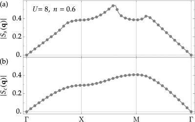
FIG. 12: Spin structure factor $S_{s}$ (a) and charge structure factor $S_{c}$ (b) for $n=0.6$, $t^{\prime}=0$, $T=0$, broadening $\eta=0.01$ for interaction $U=8$ on the high symmetry path $\Gamma$–X–M–$\Gamma$.

The spin and charge structure factors at $T=0$ are obtained as

$$S_{s,c}({\bm{q}})=-\int_{0}^{\infty}\frac{d\omega}{\pi}\operatorname{Im}\chi_{s,c}({\bm{q}},\omega+i\eta).$$ (18)

The structure factors at $n=0.6$ , $t^{\prime}=0$, and $U=8$ are shown along the path $\Gamma$–X–M–$\Gamma$ in the Brillouin zone in Fig. 12.

Similar to $\operatorname{Im}\chi_{s}({\bm{q}},\omega\rightarrow 0)$ the spin structure factor is enhanced at ${\bm{q}}=(\pi,0.625\pi)$, reflecting the upcoming magnetic instability at larger $U$. Due to the integration over $\omega$ the structure factors do not necessarily have to resemble the corresponding susceptibilities in one distinct frequency range.

III.5 Comparison with DMET-Results

Zheng et al. computed the ground-state of the Hubbard model on the square lattice in 2D Zheng and Chan (2016) by employing DMET using clusters of up to 16 sites. They report competition between inhomogeneous charge, spin, and pairing states at low doping. In the following, we compare their results with our results from slave-boson theory.

III.5.1 Results at half filling

Fig. 13 (a) and (b) compare the energy per site, double occupancy and staggered magnetization of the AFM obtained by Auxiliary-Field Quantum Monte Carlo (AFQMC), DMET and SRIKR for $t^{\prime}=0$ and different $U$ at half filling. While we find very good agreement for the double occupancy, the magnetization deviates considerably for increasing interaction. For $U\rightarrow\infty$ we find the fully magnetized Neel state with $m_{\text{SRIKR}}=1/2$ within the SRIKR slave-boson analysis whereas the magnetization saturates at $m_{\text{DMET}}\approx 0.33$ within DMET, close to the exact Heisenberg value in 2D which is given by $0.307$ according to Quantum Monte Carlo (QMC) calculations Sandvik (1997). This overestimation of the magnetization coincides with an increased energy per site in SRIKR compared to the other methods for large $U$. We expect the magnetization to be decreased by fluctuation corrections to the magnetic mean field, which are however beyond the scope of the present work.

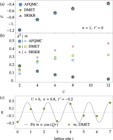
FIG. 13: Energy per site (a), double occupancy $d^{2}$ and magnetization (b) for half filling, $t^{\prime}=0$ and different $U$. We compare the results obtained from AFQMC and DMET by Zheng et al. Zheng and Chan (2016) with our SRIKR slave-boson results; (c) Local magnetization as a function of the lattice site [assuming $(\pi,Q)$ order on a $2\times 8$ cluster] for $n=0.8$, $t^{\prime}=-0.2$ and $U=6$ within DMET Zheng and Chan (2016). SRIKR yields ${\bm{Q}}\approx(\pi,0.71\pi)$, implying a spin profile of $m\propto\cos(Qr)$ which fits very well to the DMET data.

III.5.2 Results for finite doping

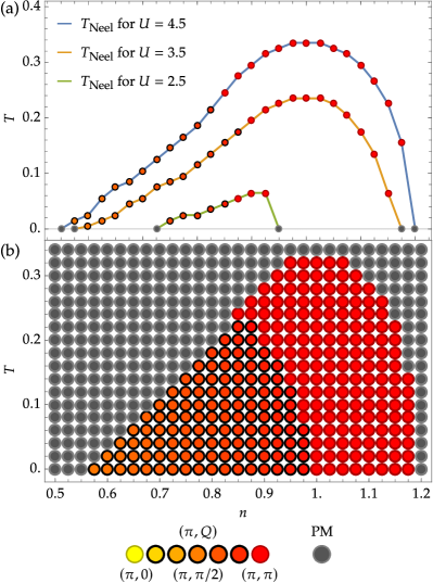
FIG. 14: (a) Transition temperature into the magnetically ordered phase versus filling $n$ for $U=2.5,3.5,4.5$ and $t^{\prime}=-0.2$. The ordering vectors on the line of the phase transition are indicated by the color of the plot markers. All presented transitions from the magnetic to the non magnetic phase are of second order; (b) Temperature dependent magnetic phase diagram for the Hubbard model for $U=4.5$ and $t^{\prime}=-0.2$. It features two distinct phases, namely the PM (gray) and the ($\pi,Q$) phase denoted by black circles filled with coloring from red to yellow. The ordering vector within one phase regime changes continuously with $U$ and $n$ visualized by the color scheme as indicated in the plot legend. The AFM is denoted by a red circle.

The domain of the $n$–$U$ SRIKR phase diagram exhibiting $(\pi,Q)$ magnetic order, is in good agreement with the DMET data given in Ref. Zheng and Chan (2016). This is exemplary shown in Fig. 13, where the spin spiral with ordering vector ${\bm{Q}}\approx(\pi,0.71\pi)$ found by SRIKR is fitted to the spin profile according to DMET on a $2\times 8$ cluster. However, in the $(Q,Q)$ domain, the ordering cannot be matched. Coincidingly, there are increasing inconsistencies between DMET clusters of size $2\times 8$ and $4\times 4$ which could be due to more severe finite size effects in the case of $(Q,Q)$ order compared to $(\pi,Q)$ order.

Moreover, we find the general trend, that points in parameter space which feature a negative compressibility within SRIKR, show highly inhomogeneous charge and/or superconducting orders according to DMET, while points with a positive compressibility are approximately homogeneous in that regard.

IV Results at finite temperature

The slave boson-mean field theory may be extended to finite temperature, provided $T$ is not too high. Although in the limit of infinite temperature the free energy is found to approach the correct limit of $F=-NT\ln 4$, the equipartition of slave bosons expected in this limit is not obtained. Rather, one finds, e.g., at half filling and for particle-hole symmetric spectrum, that $d=e=0$, for any $U>0$ with $T\rightarrow\infty$. We expect the slave boson mean field theory to be applicable up to temperatures of the order of the band width $W$.  In this section, we discuss the temperature dependence of the slave-boson mean field and fluctuation results.

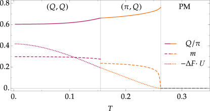
FIG. 15: Ordering wave vector component $Q$, magnetization $m=p_{0}p$ and relative difference of the magnetic free energy at ordering vector $\bm{Q}$ and paramagnetic free energy versus temperature $T$ for $U=10$, filling $n=0.8$ and $t^{\prime}=-0.2$. The vertical grid lines indicate phase transitions, the respective phases are denoted in the upper part of the plot. Near $T=0.155$ occurs a first order phase transition from $(Q,Q)$ to $(\pi,Q)$, indicated by the discontinuity in the magnetization $m$.

IV.1 Magnetic mean field phase diagram

Fig. 14b shows the temperature dependent slave-boson mean field phase diagram at $U=4.5$  and $t^{\prime}=-0.2$. In the presented temperature range we have $T\lesssim W(U)$, the renormalized bandwidth. The paramagnetic second order phase boundary coincides with results obtained from a temperature dependent fluctuation analysis of magnetic instabilities. At stronger interaction the transition into the $(\pi,\pi)-$state becomes a first order transition, which is presumably an artifact of the mean field approximation. We determined the transition temperature signaling the instability of the paramagnetic phase by first finding the root of the inverse susceptibility $1/\chi_{s}({\bm{Q}},0)$ as a function of temperature defined by $T_{c}({\bm{Q}})$ and then determining the maximum $T_{c}=\max_{{\bm{Q}}}\{T_{c}({\bm{Q}})\}$. The transition temperatures into the ordered phase so determined as a function of doping are shown in Fig. 14a, for $t^{\prime}=-0.2$ and $U=2.5,3.5,4.5$. Our results also show that a change in temperature leads to a continuous variation of the ordering vector $Q$ and can induce a first order phase transition between a $(Q,Q)$ and $(\pi,Q)$ ordering as illustrated in Fig. 15, for $n=0.8$, $t^{\prime}=-0.2$, and $U=10$, where also the magnetization and the free energy are shown. For not too small $U\gtrsim 3$ the Neel temperature has its maximum around half filling and decreases with (hole- or electron) doping.

IV.2 Critical Exponent

Furthermore we present the critical exponent $\gamma$ at the phase transition defined as

$$\chi_{s}({\bm{Q}},0)\propto(T-T_{c})^{-\gamma},$$ (19)

where ${\bm{Q}}$ is the ordering vector determined at $T_{c}$ featuring the lowest free energy in mean field approximation. Fig. 16 shows $\chi_{s}({\bm{Q}},0)^{-1}$ around the phase transition, which is situated at the sign change of the reciprocal susceptibility for ${\bm{q}}={\bm{Q}}$ and two neighboring ordering vectors. Note that ${\bm{q}}={\bm{Q}}$ features the highest $T_{c}$. The reciprocal susceptibility $\chi_{s}({\bm{Q}},0)^{-1}$ scales linearly in $T$ as shown by the comparison with the straight line in the inset, resulting in a critical exponent of $\gamma=1$.

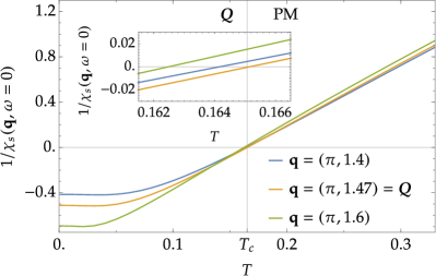
FIG. 16: Inverse static spin susceptibility for $U=12$, $t^{\prime}=0$, filling $n=0.6$ for different ${\bm{q}}$ as function of temperature in the zero frequency limit. The inset shows the vicinity of $1/\chi_{s}({\bm{q}},\omega=0)$ around the critical temperature $T_{c}=0.165$. The vertical grid line indicates the magnetic phase transition.

IV.3 Dynamical conductivity

The temperature dependence of the DC resistivity $\rho(T)=1/\sigma(T)$ at $n=0.5$, two values of interaction $U=(0,35)$ and $t^{\prime}=0$ is shown in Fig. 17a. For $T\ll W$, $\rho(T)$ follows the behavior

$$\rho(T)=\rho_{0}+A\cdot T^{2},$$ (20)

where $\rho_{0}$ and $A$ are temperature independent functions of filling, interaction and hopping parameters (for $\rho_{0}$ see the discussion given above). For large $U$, we find that the coefficient $A$ of the quadratic term is proportional to $(m^{\ast}/m_{0})^{2}\propto 1/(z_{0})^{4}$, reminiscent of what is observed in heavy fermion compounds (Kadowaki-Woods relation), as shown in Fig. 17b at $n=0.5$ and $t^{\prime}=0$. The density dependence of $A$ is weak, see Fig. 17c.

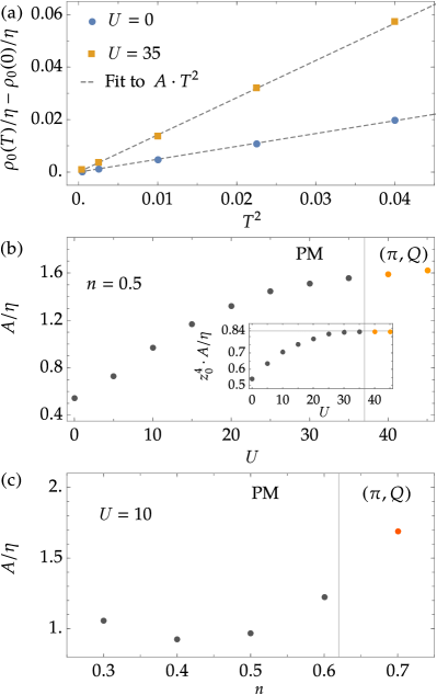
FIG. 17: (a) Temperature dependence of the resistivity $[\rho(T)-\rho(T=0)]$ versus $T^{2}$ at filling $n=0.5$, $t^{\prime}=0$ for $U=0$ (blue plot marker) and $U=35$ (orange plot marker). (b) Coefficient $A$ versus interaction $U$ for filling $n=0.5$ and $t^{\prime}=0$. The Inset shows the normalized coefficient $Az_{0}^{4}$, for large interactions the Kadowaki-Woods ratio $A\propto(m/m^{*})^{2}$ is fulfilled. The vertical grid line indicates the magnetic phase transition. The color of the plot makers display the value of the ordering vector (compare Fig. 1). (c) Coefficient $A$ versus doping $n$ for $U=10$, $t^{\prime}=0$. The vertical grid line indicates the magnetic phase transition. The color of the plot makers display the value of the ordering vector (compare Fig. 1).

IV.4 T–U phase diagram at half filling

The phase diagram in the temperature-interaction plane at half-filling is shown in Fig. 18, at $t^{\prime}=1/\sqrt{3}$. For given lower temperature, $T\lesssim 0.38$ and increasing $U$ the metallic paramagnet is entering an insulating antiferromagnetic phase and eventually a paramagnetic Mott insulator. both transitions are of first order. At low temperatures $T\lesssim 0.13$ a narrow region of metallic magnetic $(Q,Q)-$phase, $Q\approx 0.57\pi$ is found between the paramagnet and the antiferromagnetic insulator. The phase transition from the paramagnet to the metallic magnetic $(Q,Q)-$phase is of second order. At high temperature, $T\geq 0.38$, the paramagnetic metal crosses over directly into the Mott insulator phase by way of a first order transition. A comparison with the results obtained for the two sublattice frustrated model ($t^{\prime}=1/\sqrt{3}$) of Rozenberg, Kotliar and Zhang using DMFT Rozenberg et al. (1994) (see Fig. 43 in Georges et al. (1996)) shows remarkable similarity at not too high temperatures even quantitatively. Only the behavior at very high temperature is not captured correctly in the slave boson MFA, in that the first order phase separation line between metal and Mott insulator does not terminate at a critical point at about $T_{\text{crit}}\approx 1.5$, as it should, but continues up to infinite temperature. This is a consequence of the fact that in MFA the slave boson occupation numbers do not assume equilibrated values for $T\rightarrow\infty$.

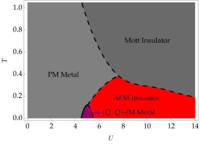
FIG. 18: Phasediagram in the $T$–$U$-plane at half filling for $t^{\prime}=1/\sqrt{3}$. It features four distinct phases: a metallic PM (gray), a Mott insulator (dark gray), a metallic magnetic phase (incommensurate ordering vector $Q\approx 0.57\pi$ (purple) and the antiferromagnetic insulating phase (red). The ordering vector is nearly constant for all parameter points in the incommensurate magnetic phase. The solid (dashed) lines indicate a phase transition of second (first) order. SB mean field yields no critical point at high $T$ which terminates the transition line of the Mott and paramagnetic metallic phase, as predicted by DMFT.

V Summary

In this paper we presented a detailed derivation of the SRIKR slave boson formalism (Sec. II and Appendix). It is shown within a path integral representation that the atomic limit is exactly recovered. The mean field theory of  spiral magnetic states is derived. The spin and charge correlation functions in the paramagnetic state are expressed in terms of the fluctuation amplitudes. We showed that the $\alpha$ constraint which fixes the number of bosons per lattice site can be enforced exactly not only on MF level, but also within the fluctuation calculation. This reduces the dimension of the fluctuation matrix $\mathcal{M}_{\mu\nu}$ by two and simplifies the calculation of the charge susceptibility compared to the formalism presented in the previous literature.

In Sec. III, results for zero temperature are presented. The solution of the mean field equations of spiral magnetic states are used to construct a phase diagram in the interaction $U$ – density $n$ plane. A number of different phases are found, characterized by the ordering wavevector ${\bm{Q}}$, classified in two types $(Q,Q)$ and $(\pi,Q)$, with $Q$ varying continuously within a given phase. The two types of phases are separated by first order transitions. We considered two hopping models: nearest neighbor hopping only ($t^{\prime}=0$) and additional next nearest neighbor hopping ($t^{\prime}=-0.2$). The $z$-factors renormalizing the hopping have been calculated and discussed in their dependence on density and interaction. The magnetization, the free energy gain of the ordered state and the ordering wave vector component $Q$ have also been evaluated. We presented the renormalized band structures in the paramagnetic and the various magnetically ordered phases. At half-filling the Mott-Hubbard transition in the paramagnetic phase, signaled by a vanishing of the $z-$factor, is preempted by the formation of magnetic antiferromagnetic order for which the $z$-factor stays finite. Examples of the Fermi surfaces in the various phases were presented as well. The compressibility in the paramagnetic phase is found to become negative in a region of the phase diagram around $n=1$, signaling an instability towards charge separation or charge order. A sign change of the compressibility happens in the magnetically ordered phase. The calculation of the charge susceptibility in the magnetically ordered phase is beyond the scope of our present work.

We calculated the spin susceptibility in the paramagnetic phase. The static spin susceptibility is parametrized in terms of a Landau interaction function $F^{a}({\bm{q}})$, found to vary in the interval $[-1,0]$, with $F^{a}({\bm{Q}})=-1$ signaling the transition to a magnetic state with ordering vector ${\bm{Q}}$. We determined the phase boundary to the magnetically ordered phase by finding the zeros of $\min_{{\bm{q}}}\{1/\chi({\bm{q}},0)\}$, the results being fully consistent with what was found from the magnetic mean field study. The dynamic spin susceptibility is parametrized in terms of a Landau damping function $\Gamma({\bm{q}},0)$, found to vary as $\Gamma\propto|{\bm{q}}|$ in the limit $|{\bm{q}}|\rightarrow 0$. At the phase transition the static spin susceptibility at the ordering wave vector is found to diverge as $\chi({\bm{Q}},0)\propto(n-n_{c})^{-\alpha}$ where $n_{c}$ is the critical doping. Surprisingly, the exponent $\alpha$ turned out to depend on whether the magnetic state was commensurate, where $\alpha\approx 1$, or incommensurate, for which $\alpha\approx 1/2$.

We calculated the charge excitation spectrum finding an interesting structure to be interpreted as two collective modes induced by interaction on top of the particle-hole continuum. The higher frequency mode has the character of an excitation into the upper Hubbard band. The mode in between the continuum and the latter mode resembles the zero sound mode of a Fermi liquid. These modes show a considerable dependence on density, interaction and on the range of hopping. The charge response function is employed to calculate the dynamical conductivity. We employed a finite imaginary part of the frequency, $\eta$, to be interpreted as an impurity scattering induced relaxation rate. The real and imaginary parts of the conductivity are found to assume Drude form, renormalized by interaction. The DC resistivity as a function of $U$ is shown to be proportional to the inverse effective mass in good approximation $\rho_{0}\propto z_{0}^{-2}$. As a function of density $n$ the relation $\rho_{0}\propto 1/(z_{0}^{2}n)$, expected to hold for the Drude conductivity is obeyed only approximately. The spin and charge structure factors were also calculated.

In Sec. IV we presented results at finite temperature. Stable solutions of the mean field equations have been found for temperatures less than the renormalized band width. We determined the magnetic phase diagram in the temperature $T$ – doping $n$ plane at fixed interaction $U$. We found the phase boundaries separating the magnetically ordered phases from the paramagnetic phase and also separating different ordered states. A continuous change of the ordering wave vector as the temperature and doping are varied is presented. The static spin susceptibility at fixed $U$ and $n$ and at the ordering vector ${\bm{Q}}$ is found to diverge at the transition as $\chi({\bm{Q}},0)\propto(T-T_{c})^{-\gamma}$, where $T_{c}$ is the critical temperature and $\gamma\approx 1$. The temperature dependent DC resistivity is shown to follow a quadratic dependence $\rho(T)=\rho_{0}+AT^{2}$. The coefficient $A$ is found to be proportional to $(m^{\ast}/m)^{2}\propto z_{0}^{-4}$, reminiscent of the Kadowaki-Woods relation found for heavy fermion compounds. Finally, we established a phase diagram in the temperature $T$ - interaction $U$ plane at half filling and choosing a next-nearest neighbor hopping parameter $t^{\prime}=1/\sqrt{3}$. The general features of the phase diagram agree very well with results obtained by other methods. The only exception is the behavior at higher temperatures, where the slave-boson mean field approximation shows a first order metal-insulator transition instead of a phase boundary ending at a critical point.

The results presented above show that the SRIKR slave-boson method is a powerful alternative to other approximate methods in the interacting fermion problem, such as DMFT, Functional Renormalization Group Method (FRG), and purely numerical methods such as QMC, Density Matrix Renormalization Group (DMRG), or DMET, to name a few prominent examples. Our method is not limited to local quantum fluctuations (like DMFT), but can describe long-range ordered phenomena. It is not limited to low to intermediate interaction (like FRG), but works for arbitrarily strong interaction, it does not suffer from a “sign problem” limiting its application to sufficiently high temperatures (like QMC), but works at low temperatures up to the bandwidth limit, it is not restricted to small systems (like DMRG and DMET), but works in the thermodynamic limit. The detailed comparison of our results with those of a recent DMET study presented in subsection III.5 demonstrates an impressive degree of compatibility as far as the fine-structure of the phasediagram at $T=0$ is concerned .

Appendix A slave-boson formalism on operator level

The slave-boson formalism was originally introduced by Kotilar and Ruckenstein Kotliar and Ruckenstein (1986) (KRSB) as a strong coupling mean field theory for a unified treatment of magnetism, metal-to-insulator transitions and Kondo physics. The method was later generalized to be manifestly spin rotation invariant Li et al. (1989); Frésard and Wölfle (1992) (SRIKR) and applied to charge and spin structure factors in the Hubbard model by means of bosonic fluctuations around the saddle point solution Li et al. (1991); Zimmermann et al. (1997). This note provides a detailed summary of spin rotation invariant slave-boson mean field formalism with fluctuations in a general notation for the Hubbard model, which can be generalized to models with one interacting and an arbitrary number of non-interacting orbitals Klett et al. (2020). We include a guide how to numerically implement the mean field equations and a section how to derive response functions from the fluctuation matrix. Moreover, we present the exact evaluation of the atomic limit in the path integral representation.

The general idea of slave-boson formalism is to define a set of bosonic operators $e_{i}$, $p_{0,i}$, ${\bm{p}}_{i}=(p_{1,i},p_{2,i},p_{3,i})$ and $d_{i}$, labeling empty, singly and doubly occupied lattice sites $i$, respectively for the interacting orbital. Spin rotation invariance requires to introduce four bosonic fields to represent a singly occupied site in comparison to two fields in the original Kotliar-Ruckenstein description. Furthermore, one needs to introduce two auxiliary fermionic fields $f_{i,\downarrow},f_{i,\uparrow}$, referred to as pseudofermions, which correspond to the quasiparticle degrees of freedom. A set of additional constraints, allows an exact mapping from the original fermionic creation and annihilation operators $(c^{\dagger},c^{\vphantom{\dagger}})$ to the slave-boson and pseudofermion fields, where the Hubbard interaction becomes bilinear, whereas hopping terms adapt a non bilinear form in bosonic operators. This way, the problem is investigated from a strong coupling perspective compared to conventional fermionic mean field theory.

The empty, singly and doubly occupied states are created by

$$\left|0\right\rangle_{i} \equiv e^{\dagger}_{i}\left|vac\right\rangle,$$ (21a)

$$\left|\sigma\right\rangle_{i} \equiv\sum\limits_{\sigma^{\prime}}p^{\dagger}_{i,\sigma\sigma^{\prime}}f^{\dagger}_{i,\sigma^{\prime}}\left|vac\right\rangle,$$ (21b)

$$\left|2\right\rangle_{i} \equiv d^{\dagger}_{i}f^{\dagger}_{i,+\frac{1}{2}}f^{\dagger}_{i,-\frac{1}{2}}\left|vac\right\rangle=d^{\dagger}_{i}f^{\dagger}_{i,\uparrow}f^{\dagger}_{i,\downarrow}\left|vac\right\rangle$$ (21c)

at each lattice site $i$ where $\sigma\in\pm\frac{1}{2}$ corresponds to the spin of the fermionic operators. The matrix operator $p^{\dagger}_{i,\sigma\sigma^{\prime}}$ will be defined in the following section. The occurring fermionic $f_{i,\sigma}$ and bosonic $b_{\alpha,i}\in\left\{e_{i},p_{0i},{\bm{p}}_{i},d_{i}\right\}$ fields fulfill the usual (anti-) commutation relations

$$\Big{\{}f^{\vphantom{\dagger}}_{i,\sigma}\ ,f^{\dagger}_{j,\sigma^{\prime}}\Big{\}} =\delta_{\sigma\sigma^{\prime}}\ \delta_{ij},$$ (22a)

$$\Big{\{}f^{\vphantom{\dagger}}_{i,\sigma}\ ,f^{\vphantom{\dagger}}_{j,\sigma^{\prime}}\Big{\}} =\Big{\{}f^{\dagger}_{i,\sigma}\ ,f^{\dagger}_{j,\sigma^{\prime}}\Big{\}}=0,$$ (22b)

$$\left[b^{\vphantom{\dagger}}_{\alpha,i}\ ,b^{\dagger}_{\beta,j}\right] =\delta_{\alpha\beta}\ \delta_{ij},$$ (22c)

$$\left[b^{\vphantom{\dagger}}_{\alpha,i}\ ,b^{\vphantom{\dagger}}_{\beta,j}\right] =\left[b^{\dagger}_{\alpha,i}\ ,b^{\dagger}_{\beta,j}\right]=0.$$ (22d)

The site index $i$ will be dropped for readability in the following, it is implied that the all equations without an additional index $i$ hold for every lattice site.

A.1 Construction of the p-Matrix

While the empty and doubly occupied states transform like scalars, the singly occupied state $\left|\sigma\right\rangle$ needs to transform like a spinor under spin rotation, consequently $p^{\dagger}_{i,\sigma\sigma^{\prime}}$ represents an element of a $2\times 2$ matrix. The total spin of the singly occupied state is $S=\frac{1}{2}$ and consists of a pseudofermionic ($S_{f}=\frac{1}{2}$) and a bosonic component. The possible bosonic spins are $S_{b}=0$ and $S_{b}=1$ yielding a scalar boson field $p_{0}$ and a vector boson field ${\bm{p}}=(p_{x},p_{y},p_{z})$ where $x,y,z$ are the Cartesian components. The spin operator for $S_{b}=1$ is given by

$$\hat{{\bm{S}}}=\begin{pmatrix}\underline{\smash{S}}^{x}\\ \underline{\smash{S}}^{y}\\ \underline{\smash{S}}^{z}\end{pmatrix},$$ (23)

where

$$\underline{\smash{S}}^{x} =\frac{1}{\sqrt{2}}\begin{pmatrix}0&1&0\\ 1&0&1\\ 0&1&0\end{pmatrix},$$ (24a)

$$\underline{\smash{S}}^{y} =\frac{1}{\sqrt{2}}\begin{pmatrix}0&-\mathrm{i}&0\\ \mathrm{i}&0&-\mathrm{i}\\ 0&\mathrm{i}&0\end{pmatrix},$$ (24b)

$$\underline{\smash{S}}^{z} =\begin{pmatrix}1&0&0\\ 0&0&0\\ 0&0&-1\end{pmatrix}.$$ (24c)

For a spin rotational invariant representation, we choose the ${\bm{p}}^{\dagger}$ operator to create a bosonic state ($S_{b}=1$) which is polarized in the $x,y$ and $z$ direction respectively with the magnetic quantum number $m=0$

$$\begin{gathered}\underline{\smash{S}}^{i}\left|\chi_{i}\right\rangle=0\\ {\bm{\chi}}_{x}=\frac{1}{\sqrt{2}}\begin{pmatrix}-1\\ 0\\ 1\end{pmatrix},\qquad{\bm{\chi}}_{y}=\frac{1}{\sqrt{2}}\begin{pmatrix}\mathrm{i}\\ 0\\ \mathrm{i}\end{pmatrix},\qquad{\bm{\chi}}_{z}=\begin{pmatrix}0\\ 1\\ 0\end{pmatrix}.\end{gathered}$$ (25)

This basis is orthonormal on the spin Hilbert space $\left\langle\chi_{i}\right|\chi_{j}\rangle=\delta_{ij}$. The relative phases of ${\bm{\chi}}_{i}$ are not arbitrary because they are related by spin rotation $\mathrm{e}^{-i{\bm{\phi}}\hat{{\bm{S}}}}$ and chosen such that

$${\bm{\chi}}_{y}=\mathrm{e}^{-i\frac{\pi}{2}\underline{\smash{S}}^{z}}{\bm{\chi}}_{x},$$ (26a)

$${\bm{\chi}}_{z}=\mathrm{e}^{-i\frac{\pi}{2}\underline{\smash{S}}^{x}}{\bm{\chi}}_{y},$$ (26b)

$${\bm{\chi}}_{x}=\mathrm{e}^{-i\frac{\pi}{2}\underline{\smash{S}}^{y}}{\bm{\chi}}_{z}.$$ (26c)

In order to add the spin of the boson and the pseudofermion, it is convenient to use the basis of eigenstates of the $\underline{\smash{S}}^{z}$ operator, which can be found as superposition of the spinors ${\bm{\chi}}_{x},{\bm{\chi}}_{y}$ and ${\bm{\chi}}_{z}$ yielding the ladder operators

$$p^{{\vphantom{\dagger}}}_{1,1} \equiv-\frac{1}{\sqrt{2}}\left(p^{{\vphantom{\dagger}}}_{x}+\mathrm{i}p^{{\vphantom{\dagger}}}_{y}\right),$$ (27a)

$$p^{{\vphantom{\dagger}}}_{1,0} \equiv p^{{\vphantom{\dagger}}}_{z}\ ,$$ (27b)

$$p^{{\vphantom{\dagger}}}_{1,-1} \equiv\frac{1}{\sqrt{2}}\left(p^{{\vphantom{\dagger}}}_{x}-\mathrm{i}p^{{\vphantom{\dagger}}}_{y}\right)\ .$$ (27c)

Consequently a state with total spin of $S=\frac{1}{2}$ composed of a $S_{f}=\frac{1}{2}$ pseudofermion $f_{\sigma^{\prime}}$ and a $S_{b}=1$ slave-boson $p_{1,m_{1}}$ is given by (Frésard and Wölfle, 1992)

$$\begin{split}\left|\sigma\right\rangle_{S={\frac{1}{2}}}&=\sum_{\sigma^{\prime}=\pm\frac{1}{2}}C\left(S_{b}=1,S_{f}=\frac{1}{2};m_{b}=\sigma-\sigma^{\prime},m_{f}=\sigma^{\prime}\Big{|}S=\frac{1}{2};\sigma\right)\ p^{\dagger}_{1,m_{b}}f^{\dagger}_{\sigma^{\prime}}\left|vac\right\rangle=\sum_{\sigma^{\prime}=\pm\frac{1}{2}}\left(p^{\dagger}_{S=1}\right)_{\sigma\sigma^{\prime}}f^{\dagger}_{\sigma^{\prime}}\left|vac\right\rangle\end{split}$$ (28)

with $\sigma=\pm\frac{1}{2}$ and the Clebsch-Gordon coefficients

$$C\left(1,\frac{1}{2};\sigma\mp\frac{1}{2},\pm\frac{1}{2}\Big{|}\frac{1}{2},\sigma\right)=\mp\sqrt{\frac{3\mp 2\sigma}{6}}.$$ (29)

As Eq. (28) implies, we can write the bosons in a convenient matrix notation $\underline{\smash{p}}_{\leavevmode\nobreak\ S=1}$, which reads

$$\underline{\smash{p}}^{\dagger}_{\leavevmode\nobreak\ S=1}=\begin{pmatrix}-\sqrt{\frac{1}{3}}p^{\dagger}_{1,0}&\sqrt{\frac{2}{3}}p^{\dagger}_{1,1}\\ -\sqrt{\frac{2}{3}}p^{\dagger}_{1,-1}&\sqrt{\frac{1}{3}}p^{\dagger}_{1,0}\end{pmatrix},$$ (30)

using the basis

$$f^{\dagger}_{\sigma^{\prime}}=\begin{pmatrix}f^{\dagger}_{\uparrow}\\ f^{\dagger}_{\downarrow}\\ \end{pmatrix}$$ (31)

for the pseudofermions. To obtain the full matrix, one has to take contributions of the scalar field $p_{0}$ as a superposition into account, which only acts diagonal on the spin subspace. Inserting Eq. (27), one finds for the full matrix

$$\underline{\smash{p}}^{\dagger}=\begin{pmatrix}ap_{0}^{\dagger}+bp^{\dagger}_{z}&b(p^{\dagger}_{x}-\mathrm{i}p^{\dagger}_{y})\\ b(p^{\dagger}_{x}+\mathrm{i}p^{\dagger}_{y})&ap_{0}^{\dagger}-bp^{\dagger}_{z}\end{pmatrix}.$$ (32)

The coefficients $a$ and $b$ are not arbitrary, but have to be chosen such that the normalization

$$\sum_{\sigma^{\prime}\sigma^{\prime\prime}}\left\langle vac\right|f^{\vphantom{\dagger}}_{\sigma^{\prime\prime}}p^{\vphantom{\dagger}}_{\sigma^{\prime\prime}\sigma}p^{\dagger}_{\sigma\sigma^{\prime}}f^{\dagger}_{\sigma^{\prime}}\left|vac\right\rangle=1$$ (33)

is fulfilled for $\sigma=\pm\frac{1}{2}$ which implies $3b^{2}+a^{2}=1$. The ratio $a/b$ is a free parameter. It can be chosen $a=b=1/2$ which finally yields

$$\underline{\smash{p}}^{\dagger} =\frac{1}{2}\sum_{\mu=0}^{3}p^{\dagger}_{\mu}\underline{\smash{\tau}}^{\mu}=\frac{1}{2}\begin{pmatrix}p^{\dagger}_{0}+p^{\dagger}_{z}&p^{\dagger}_{x}-\mathrm{i}p^{\dagger}_{y}\\ p^{\dagger}_{x}+\mathrm{i}p^{\dagger}_{y}&p^{\dagger}_{0}-p^{\dagger}_{z}\end{pmatrix},$$ (34a)

$$\underline{\smash{p}}^{\vphantom{\dagger}} =\frac{1}{2}\sum_{\mu=0}^{3}p_{\mu}\underline{\smash{\tau}}^{\mu}=\frac{1}{2}\begin{pmatrix}p^{{\vphantom{\dagger}}}_{0}+p_{z}&p^{{\vphantom{\dagger}}}_{x}-\mathrm{i}p^{{\vphantom{\dagger}}}_{y}\\ p^{{\vphantom{\dagger}}}_{x}+\mathrm{i}p_{y}&p^{{\vphantom{\dagger}}}_{0}-p^{{\vphantom{\dagger}}}_{z}\end{pmatrix}$$ (34b)

where $\underline{\smash{\tau}}^{\mu}$ is the vector of the Pauli matrices, including the identity matrix $\underline{\smash{\tau}}^{0}\equiv\underline{\smash{\mathbbm{1}}}_{2}$. The commutator of these matrix operators is given by

$$\left[p_{\sigma_{1}\sigma_{2}},p_{\sigma_{3}\sigma_{4}}^{\dagger}\right]=\frac{1}{2}\delta_{\sigma_{1}\sigma_{4}}\delta_{\sigma_{2}\sigma_{3}}.$$ (35)

A.2 slave-boson representation and time reversal properties

The original, fermionic operators $c^{\dagger}_{\sigma},c^{\vphantom{\dagger}}_{\sigma}$, are mapped to the slave-boson operators by

$$c^{\dagger}_{\sigma} \equiv\sum_{\sigma^{\prime}}z^{\dagger}_{\sigma\sigma^{\prime}}f^{\dagger}_{\sigma^{\prime}},$$ (36a)

$$c^{\vphantom{\dagger}}_{\sigma} \equiv\sum_{\sigma^{\prime}}f^{{\vphantom{\dagger}}}_{\sigma^{\prime}}z^{{\vphantom{\dagger}}}_{\sigma^{\prime}\sigma},$$ (36b)

with

$$z_{\sigma\sigma^{\prime}} =e^{\dagger}p_{\sigma\sigma^{\prime}}+\tilde{p}^{\dagger}_{\sigma\sigma^{\prime}}d,$$ (37a)

$$z^{\dagger}_{\sigma\sigma^{\prime}} =p^{\dagger}_{\sigma\sigma^{\prime}}e+d^{\dagger}\tilde{p}^{\vphantom{\dagger}}_{\sigma\sigma^{\prime}},$$ (37b)

and

$$\tilde{p}_{\sigma\sigma^{\prime}}=\frac{1}{2}\left(p_{0}\tau^{0}_{\sigma\sigma^{\prime}}-\sum_{\mu=1}^{3}p^{\mu}_{\sigma\sigma^{\prime}}\right)$$ (38a)

or equivalently

$$\tilde{p}_{\sigma\sigma^{\prime}}=4\sigma\sigma^{\prime}p_{-\sigma^{\prime}-\sigma}\qquad\sigma\in\Bigg{\{}\frac{1}{2},-\frac{1}{2}\Bigg{\}}.$$ (38b)

Note, that In this notation $-\sigma$ corresponds to a spin flip.

Eq. (36) is straight forward to understand when acting on an empty or doubly occupied site. For single occupation, there are two states because of the spin, which makes the situation slightly more complicated and it is necessary to define $\tilde{{\bm{p}}}$ in order to obtain the expected result

$$\begin{split}c^{\dagger}_{\sigma}\left|\sigma^{\prime}\right\rangle&=\sum_{\sigma_{1}\sigma_{2}}z^{\dagger}_{\sigma\sigma_{1}}f^{\dagger}_{\sigma_{1}}p^{\dagger}_{\sigma^{\prime}\sigma_{2}}f^{\dagger}_{\sigma_{2}}\left|vac\right\rangle\\ &=2\sigma\delta_{-\sigma\sigma^{\prime}}d^{\dagger}f^{\dagger}_{\uparrow}f^{\dagger}_{\downarrow}\left|vac\right\rangle=2\sigma\delta_{-\sigma\sigma^{\prime}}\left|2\right\rangle.\end{split}$$ (39)

Eq. (36) fulfills the expected behavior under time reversal. Fermionic operators need to fulfill

$$\hat{T}c^{\vphantom{\dagger}}_{\uparrow}\hat{T}^{-1} =c^{\vphantom{\dagger}}_{\downarrow},$$ (40a)

$$\hat{T}c^{\vphantom{\dagger}}_{\downarrow}\hat{T}^{-1} =-c^{\vphantom{\dagger}}_{\uparrow}$$ (40b)

where $\hat{T}$ is the time reversal operator. Since $p_{0}$ annihilates a spin singlet and ${\bm{p}}$ a spin triplet, we expect $p_{0}$ to be even, $\hat{T}p_{0}\hat{T}^{-1}=p_{0}$ and ${\bm{p}}$ to be odd $\hat{T}{\bm{p}}\hat{T}^{-1}=-{\bm{p}}$ under time reversal. Moreover, the operator $\hat{T}$ is anti-unitary $\hat{T}i\hat{T}^{-1}=-i$. The properties of the other slave-boson fields under time reversal can now be determined demanding that Eq. (40) holds within slave-boson formalism

$$\hat{T}p_{0}\hat{T}^{-1} =p_{0},$$ (41a)

$$\hat{T}{\bm{p}}\hat{T}^{-1} =-{\bm{p}},$$ (41b)

$$\hat{T}e\hat{T}^{-1} =e,$$ (41c)

$$\hat{T}d\hat{T}^{-1} =d,$$ (41d)

$$\hat{T}f_{\uparrow}\hat{T}^{-1} =f_{\downarrow},$$ (41e)

$$\hat{T}f_{\downarrow}\hat{T}^{-1} =-f_{\uparrow}.$$ (41f)

A.3 Constraints in slave-boson formalism

In order to have an exact mapping of original fermionic operators to slave-boson operators, one needs to enforce the following constraints to recover from the extended Fock space to the physical Hilbert space

$$1 =e^{\dagger}e+d^{\dagger}d+\sum_{\mu=0}^{3}p^{\dagger}_{\mu}p^{{\vphantom{\dagger}}}_{\mu}$$ (42a)

$$f^{\dagger}_{\sigma^{\prime}}f^{{\vphantom{\dagger}}}_{\sigma\vphantom{{}^{\prime}}} =2\sum_{\sigma_{1}}p^{\dagger}_{\sigma_{1}\sigma}p^{{\vphantom{\dagger}}}_{\sigma^{\prime}\sigma_{1}}+\delta_{\sigma\sigma^{\prime}}d^{\dagger}d.$$ (42b)

Eq. (42b) can be rewritten in terms of $$p_{\mu} \sum_{\sigma\sigma^{\prime}}\tau^{\mu}_{\sigma\sigma^{\prime}}$$’s to four scalar equations by expanding in Pauli matrices including the identity matrix, i.e. applying on both sides of the equation

$$\sum_{\sigma}f^{\dagger}_{\sigma}f^{\vphantom{\dagger}}_{\sigma} =\sum_{\mu=0}^{3}p^{\dagger}_{\mu}p^{{\vphantom{\dagger}}}_{\mu}+2d^{\dagger}d$$ (42c)

$$\sum_{\sigma\sigma^{\prime}}{\bm{\tau}}_{\sigma\sigma^{\prime}}f^{\dagger}_{\sigma^{\prime}}f^{\vphantom{\dagger}}_{\sigma\vphantom{{}^{\prime}}} =p^{\dagger}_{0}{\bm{p}}+{\bm{p^{\dagger}}}p_{0}-\mathrm{i}{\bm{p^{\dagger}}}\times{\bm{p}}\;.$$ (42d)

These constraints are enforced on each lattice site. The first constraint Eq. (42a) makes sure that every site is occupied by exactly one slave-boson. The second constraint Eq. (42c) matches the number of pseudofermions and slave-bosons according to Eq. (21). The third constraint Eq. (42d) relates the spin of the pseudofermions and slave-bosons which are not independent as Eq. (28) indicates. It states that a spin flip in pseudofermions can be recast as a spin flip in the slave-bosons. Since such a recast spin flip has to obey the previous assignment of $p$-bosons and pseudofermions one has to employ the third constraint .

The necessity of the constraints can be seen mathematically by calculating the anti-commutator $\{c^{\vphantom{\dagger}}_{\sigma\vphantom{{}^{\prime}}},c^{\dagger}_{\sigma^{\prime}}\}=\delta_{\sigma\sigma^{\prime}}$ in slave-boson formalism, which is only recovered correctly when applying all of the constraints. It is sufficient to verify the commutator on the physical subspace. This way, one can exploit, that two bosonic annihilation operators to the very right side of an equation annihilate any state because of Eq. (42a). Such an ordering can be achieved by using Eq. (38b) and the commutator Eq. (35). Moreover, the pseudofermions can be replaced by slave-boson operators by means of the second constraint Eq. (42b). It turns out that only terms which are bilinear in bosonic operators remain

$$\begin{gathered}\Big{\{}c^{\vphantom{\dagger}}_{\sigma\vphantom{{}^{\prime}}}\ ,c^{\dagger}_{\sigma^{\prime}}\Big{\}}=\sum_{\sigma_{1}\sigma_{2}}\left(f^{\vphantom{\dagger}}_{\sigma_{1}}z^{\vphantom{\dagger}}_{\sigma_{1}\sigma}z^{\dagger}_{\sigma^{\prime}\sigma_{2}}f^{\dagger}_{\sigma_{2}}+z^{\dagger}_{\sigma^{\prime}\sigma_{2}}f^{\dagger}_{\sigma_{2}}f^{\vphantom{\dagger}}_{\sigma_{1}}z^{\vphantom{\dagger}}_{\sigma_{1}\sigma}\right)\\ =\delta_{\sigma\sigma^{\prime}}\left(e^{\dagger}e+d^{\dagger}d\right)+2\sum_{\sigma_{1}}\left(4\sigma\sigma^{\prime}p^{\dagger}_{-\sigma\sigma_{1}}p^{\vphantom{\dagger}}_{\sigma_{1}-\sigma^{\prime}}+p^{\dagger}_{\sigma^{\prime}\sigma_{1}}p^{\vphantom{\dagger}}_{\sigma_{1}\sigma}\right).\end{gathered}$$ (43a)

The second term in Eq. (43a) can be further decomposed

$$\begin{gathered}\sum_{\sigma_{1}}p^{\dagger}_{\sigma^{\prime}\sigma_{1}}p^{\vphantom{\dagger}}_{\sigma_{1}\sigma}=\frac{1}{4}\sum_{\mu=0}^{3}p^{\dagger}_{\mu}p^{\vphantom{\dagger}}_{\mu}\delta_{\sigma\sigma^{\prime}}\\ +\frac{1}{4}\sum_{\mu=1}^{3}\tau^{\mu}_{\sigma^{\prime}\sigma}\left(p^{\dagger}_{\mu}p^{\vphantom{\dagger}}_{0}+p_{0}^{\dagger}p^{\vphantom{\dagger}}_{\mu}\right)+\frac{i}{4}\sum_{\mu\mu^{\prime}\nu=1}^{3}\epsilon^{\ \mu\mu^{\prime}\nu}\tau^{\nu}_{\sigma\sigma^{\prime}}p^{\dagger}_{\mu}p^{\vphantom{\dagger}}_{\mu^{\prime}}\end{gathered}$$ (43b)

Now, making use of

$$\tau^{\mu}_{\sigma^{\prime}\sigma}=-4\sigma\sigma^{\prime}\tau^{\mu}_{-\sigma-\sigma^{\prime}},\quad\mu\in\{1,2,3\}$$ (43c)

all terms containing Pauli matrices vanish in Eq. (43a) which yields

$$\Big{\{}c^{\vphantom{\dagger}}_{\sigma\vphantom{{}^{\prime}}}\ ,c^{\dagger}_{\sigma^{\prime}}\Big{\}}=\delta_{\sigma\sigma^{\prime}}\left(e^{\dagger}e+d^{\dagger}d+\sum_{\mu=0}^{3}p^{\dagger}_{\mu}p^{\vphantom{\dagger}}_{\mu}\right)=\delta_{\sigma\sigma^{\prime}}$$ (43d)

and leads to the expected result by once more using the first constraint. Consequently, the fermionic character of the fields is preserved in slave-boson formalism.

Note, that pseudofermions can be replaced by slave-bosons every time they appear bilinear with Eq. (42b). However, a combination of pseudofermions on different sites cannot be replaced.

The constraints can be enforced by means adequate projection operators. We define

$$A \equiv e^{\dagger}e+d^{\dagger}d+\sum_{\mu=0}^{3}p^{\dagger}_{\mu}p^{\vphantom{\dagger}}_{\mu}-1$$ (44a)

$$B_{0} \equiv\sum_{\mu=0}^{3}p^{\dagger}_{\mu}p^{\vphantom{\dagger}}_{\mu}+2d^{\dagger}d-\sum_{\sigma}f^{\dagger}_{\sigma}f^{\vphantom{\dagger}}_{\sigma}$$ (44b)

$${\bm{B}} \equiv p^{\dagger}_{0}{\bm{p}}+{\bm{p}}^{\dagger}p^{\vphantom{\dagger}}_{0}-\mathrm{i}{\bm{p}}^{\dagger}\times{\bm{p}}-\sum_{\sigma\sigma^{\prime}}{\bm{\tau}}_{\sigma\sigma^{\prime}}f^{\dagger}_{\sigma^{\prime}}f^{{\vphantom{\dagger}}}_{\sigma}$$ (44c)

and need to enforce $A=B_{0}={\bm{B}}=0$ in order to fulfill the constraints. To do so, we define the following projection operators:

$$\mathcal{P}_{\alpha} =\frac{1}{2\pi T}\int_{-\pi T}^{\pi T}\mathrm{e}^{i\alpha A/T}d\alpha=\delta_{A,0}$$ (45a)

$$\mathcal{P}_{\beta_{0}} =\frac{1}{2\pi T}\int_{-\pi T}^{\pi T}\mathrm{e}^{iB_{0}Y/T}d\beta_{0}=\delta_{B_{0},0}$$ (45b)

$$\mathcal{P}_{{\bm{\beta}}} =\lim_{N\rightarrow\infty}\frac{1}{(2\pi NT)^{3}}\iiint_{-\pi NT}^{\pi NT}\prod_{i=1}^{3}\mathrm{e}^{i{\bm{\beta}}_{i}B_{i}/T}d\beta_{i}=\delta_{{\bm{B}},0}$$ (45c)

$$\mathcal{P} \equiv\mathcal{P}_{\alpha}\mathcal{P}_{\beta_{0}}\mathcal{P}_{{\bm{\beta}}}.$$ (45d)

Note that, since ${\bm{Z}}$ contains operators which are not number operators, its eigenvalues may have non integer values. Therefore the integral has to be extended to infinity to project out all unphysical states. The partition function of the physical subspace for a Hamiltonian $H$ is then given by

$$Z_{\text{eff}}=\operatorname{tr}\left[e^{-H/T}\mathcal{P}\right].$$ (46)

The constraints commute with the slave-boson representation of fermionic creation (annihilation) operators

$$\left[\sum_{\sigma^{\prime}}z^{\dagger}_{\sigma\sigma^{\prime}}f^{\dagger}_{\sigma^{\prime}}\ ,\ A\right]=\left[\sum_{\sigma^{\prime}}z^{\dagger}_{\sigma\sigma^{\prime}}f^{\dagger}_{\sigma^{\prime}}\ ,\ B_{0}\right]=\left[\sum_{\sigma^{\prime}}z^{\dagger}_{\sigma\sigma^{\prime}}f^{\dagger}_{\sigma^{\prime}}\ ,\ {\bm{B}}\right]=0$$ (47a)

$$\left[\sum_{\sigma^{\prime}}f^{{\vphantom{\dagger}}}_{\sigma^{\prime}}z^{{\vphantom{\dagger}}}_{\sigma^{\prime}\sigma}\ ,\ A\right]=\left[\sum_{\sigma^{\prime}}f^{{\vphantom{\dagger}}}_{\sigma^{\prime}}z^{{\vphantom{\dagger}}}_{\sigma^{\prime}\sigma}\ ,\ B_{0}\right]=\left[\sum_{\sigma^{\prime}}f^{{\vphantom{\dagger}}}_{\sigma^{\prime}}z^{{\vphantom{\dagger}}}_{\sigma^{\prime}\sigma}\ ,\ {\bm{B}}\right]=0.$$ (47b)

Consequently, the constraints commute with any reasonable Hamiltonian in second quantisazion

$$\left[H,A\right]=\left[H,B_{0}\right]=\left[H,{\bm{B}}\right]=0$$ (48)

and with the time evolution operator, i.e. a state on the physical subspace cannot propagate into an unphysical state.

A.4 Operators in slave-boson formalism

This section summarizes important fermionic operators and their representation in slave-boson formalism.

A.4.1 Spin density operator

The spin density operator in fermionic language is given by

$$\hat{{\bm{S}}}=\frac{1}{2}\sum\limits_{\sigma\sigma^{\prime}}c^{\dagger}_{\sigma}\bm{\tau}^{\vphantom{\dagger}}_{\sigma\sigma^{\prime}}c^{{\vphantom{\dagger}}}_{\sigma^{\prime}}$$ (49a)

Within slave-boson formalism, one finds

$$\begin{split}\hat{{\bm{S}}}&=\frac{1}{2}\sum\limits_{\sigma\sigma^{\prime}\sigma_{1}\sigma_{2}}z^{\dagger}_{\sigma\sigma_{1}}f^{\dagger}_{\sigma_{1}}\bm{\tau}^{\vphantom{\dagger}}_{\sigma\sigma^{\prime}}z^{{\vphantom{\dagger}}}_{\sigma_{2}\sigma^{\prime}}f^{{\vphantom{\dagger}}}_{\sigma_{2}}\\ &=\sum\limits_{\sigma\sigma^{\prime}\sigma_{1}}p^{\dagger}_{\sigma\sigma_{1}}\bm{\tau}^{\vphantom{\dagger}}_{\sigma\sigma^{\prime}}p^{{\vphantom{\dagger}}}_{\sigma_{1}\sigma^{\prime}}\\ &=\frac{1}{4}\sum_{\mu\mu^{\prime}=0}^{3}p^{\dagger}_{\mu^{\prime}}p^{{\vphantom{\dagger}}}_{\mu}\sum_{\sigma\sigma^{\prime}\sigma_{1}}\tau^{\mu}_{\sigma_{1}\sigma^{\prime}}{\bm{\tau}}^{\vphantom{\dagger}}_{\sigma\sigma^{\prime}}\tau^{\mu^{\prime}}_{\sigma\sigma_{1}}\\ &=\frac{1}{2}\left(p^{\dagger}_{0}\check{{{\bm{p}}}}+\check{{\bm{p}}}^{\dagger}p_{0}-i\check{{\bm{p}}}^{\dagger}\times\check{{{\bm{p}}}}\right)\end{split}$$ (49b)

with

$$\check{{\bm{p}}}=(p_{1},-p_{2},p_{3})^{T}.$$ (49c)

It is easy to verify that this representation fulfills the spin algebra $$\left[\hat{S}_{i},\hat{S}_{j}\right]=i\epsilon_{ijk}\hat{S}_{k}$$.

A.4.2 Density operator

The fermionic density operator of the interacting electrons is defined by

$$\hat{n}=\sum_{\sigma}c^{\dagger}_{\sigma}c^{\vphantom{\dagger}}_{\sigma}.$$ (50a)

Replacing the $$p$$-bosons with the second constraint Eq. (42b) yields

$$\hat{n} =\sum_{\sigma}f^{\dagger}_{\sigma}f^{{\vphantom{\dagger}}}_{\sigma},$$ (50b)

i.e. the number of original fermions matches the number of pseudofermions. Using the constraints, it can also be written by means of slave-bosons only

$$\hat{n}=1+d^{\dagger}d-e^{\dagger}e.$$ (50c)

A.4.3 Hubbard interaction operator

The Hubbard interaction is defined by

$$\hat{U}=Uc^{\dagger}_{\uparrow}c^{\vphantom{\dagger}}_{\uparrow}c^{\dagger}_{\downarrow}c^{\vphantom{\dagger}}_{\downarrow}.$$ (51a)

It is translated to slave-boson formalism by using the transformation property of the density operator Eq. (50b)

$$\begin{split}\hat{U}=Uf^{\dagger}_{\sigma}f^{\vphantom{\dagger}}_{\sigma}f^{\dagger}_{-\sigma}f^{\vphantom{\dagger}}_{-\sigma}=Ud^{\dagger}d.\end{split}$$ (51b)

The Hubbard interaction becomes bilinear, which is why a consecutive mean field treatment is well adapted for strong coupling.

Appendix B Path Integral formulation of slave-boson formalism

Our goal is to derive the partition function which will be used to calculate thermodynamic quantities on mean field level and correlation functions by means of fluctuations around the mean field solution. It is given by the path integral over coherent states with imaginary time propagation Negele and Orland (1988)

$$Z=\int\mathcal{D}\left[f^{*},f\right]\mathcal{D}\left[\psi^{*},\psi\right]\mathrm{e}^{-\mathcal{S}\left[(f^{*},f),(\psi^{*},\psi)\right]}$$ (52a)

where

$$\mathcal{S}\left[(f^{*},f),(\psi^{*},\psi)\right]=\int_{0}^{\frac{1}{T}}\mathcal{L}\left[(f^{*}_{\tau},f^{\vphantom{\dagger}}_{\tau}),(\psi^{*}_{\tau},\psi^{\vphantom{\dagger}}_{\tau})\right]\ d\tau$$ (52b)

is the action and $\mathcal{L}$ the Lagrangian. In the path integral, the operators are replaced by their coherent state eigenvalues, which are complex (Grassmann) numbers for the slave-bosons (pseudofermions) represented by $\psi_{\tau}$ ($f_{\tau})$ at imaginary time $\tau$. Moreover, $T$ is the temperature and $\mathcal{D}\left[\psi^{*},\psi\right]$ ($\mathcal{D}\left[f^{*},f\right]$) represents the integration over all field configurations.

The constraints can be enforced by means of the projectors defined in Eq. (45). Since the they commute with the Hamiltonian on operator level, the physical subspace is recovered with the following effective Lagrangian, featuring time independent Lagrange multipliers.

$$Z_{\text{eff}}=\lim_{N\rightarrow\infty}\frac{1}{(2\pi T)^{2}}\frac{1}{(2\pi NT)^{3}}\int_{-\pi T}^{\pi T}\mathrm{d}\alpha\int_{-\pi T}^{\pi T}\mathrm{d}\beta_{0}\iiint_{-\pi NT}^{\pi NT}\mathrm{d}^{3}\beta\int\mathcal{D}[f^{*},f]\mathcal{D}[\psi^{*},\psi]\mathrm{e}^{-\mathcal{S}_{\text{eff}}\left[(f^{*},f),(\psi^{*},\psi),\alpha,\beta_{0},{\bm{\beta}}\right]}$$ (53a)

$$\text{with}\quad\mathcal{L}_{\text{eff}}=\mathcal{L}+\mathrm{i}(\alpha A+\beta_{0}B_{0}+{\bm{\beta}}{\bm{B}})$$ (53b)

B.1 Effective Lagrangian in momentum space

A general one band Hubbard Hamiltonian is give by

$$H=\sum_{ij}\sum_{\sigma\sigma^{\prime}}c^{\dagger}_{i,\sigma}t_{ij}\,c^{{\vphantom{\dagger}}}_{j,\sigma}-\mu_{0}\sum_{i}\hat{n}_{i}+U\sum_{i}c_{i,\uparrow}^{\dagger}c^{\vphantom{\dagger}}_{i,\uparrow}c^{\dagger}_{i,\downarrow}c_{i,\downarrow}^{\vphantom{\dagger}}$$ (54a)

$$=\sum_{{\bm{k}}}{\bm{c}}^{\dagger}_{{\bm{k}}}\underline{\smash{\mathcal{H}}}_{\bm{k}}{\bm{c}}^{\vphantom{\dagger}}_{\bm{k}}-\mu_{0}\sum_{i}\hat{n}_{i}+U\sum_{i}c_{i,\uparrow}^{\dagger}c^{\vphantom{\dagger}}_{i,\uparrow}c^{\dagger}_{i,\downarrow}c_{i,\downarrow}^{\vphantom{\dagger}}.$$ (54b)

The tensor $t_{ij}$ may contain arbitrary hopping amplitudes. Moreover, we define the density operator $\hat{n}_{i}=\sum_{\sigma}c^{\dagger}_{i,\sigma}c^{\vphantom{\dagger}}_{i,\sigma}$, $\mu_{0}$ is the chemical potential and $U$ is the on-site Hubbard interaction strength.

By Fourier transformation, the Hamiltonian can be rewritten as in Eq. (54b) where ${\bm{c}}_{\bm{k}}\equiv(c_{1,{\bm{k}},\uparrow},c_{1,{\bm{k}},\downarrow})^{T}$ is to be understood as a $2$-dimensional spinor and $\underline{\smash{\mathcal{H}}}_{\bm{k}}$ is the $2\times 2$ bare hopping matrix.

The Hamiltonian can be rewritten using the slave-boson representation given in Eq. (36) and the representation of the operators given by Eq. (50b) and Eq. (51b). The effective Lagrangian within path integral formulation after Fourier transformation of $z^{\dagger}_{i},\ f^{*}_{i},\ z^{\vphantom{\dagger}}_{j}$ and $\ f^{\vphantom{\dagger}}_{j}$ is given by

$$\begin{gathered}\mathcal{L}_{\text{eff}}[f,\psi]=\mathcal{L}_{\mathrm{F}}[f,\psi]+\mathcal{L}_{\mathrm{B}}[\psi]=\sum_{{\bm{k}}_{1},{\bm{k}}_{2}}{\bm{f}}_{{\bm{k}}_{1}}^{\dagger}\left(\partial\tau+\underline{\smash{H}}_{{\bm{k}}_{1},{\bm{k}}_{2}}[\psi]\right){\bm{f}}_{{\bm{k}}_{2}}^{\vphantom{\dagger}}\\ +\sum_{i}\Bigg{[}d^{*}_{i}(\partial_{\tau}+U)d^{\vphantom{\dagger}}_{i}+e^{*}_{i}\partial_{\tau}e^{\vphantom{\dagger}}_{i}+{\bm{p}}^{*}_{i}\partial_{\tau}{\bm{p}}^{\vphantom{\dagger}}_{i}+i\alpha_{i}\left(e^{*}_{i}e^{\vphantom{\dagger}}_{i}+p^{*}_{0,i}p^{\vphantom{\dagger}}_{0,i}+{\bm{p}}^{*}_{i}\cdot{\bm{p}}^{\vphantom{\dagger}}_{i}+d^{*}_{i}d^{\vphantom{\dagger}}_{i}-1\right)\\ -i\beta_{0,i}\left(p^{*}_{0,i}p^{\vphantom{\dagger}}_{0,i}+{\bm{p}}^{*}_{i}\cdot{\bm{p}}^{\vphantom{\dagger}}_{i}+2d^{*}_{i}d^{\vphantom{\dagger}}_{i}\right)-i{\bm{\beta}}_{i}\cdot\left(p_{0,i}^{*}{\bm{p}}_{i}^{\vphantom{\dagger}}+{\bm{p}}^{*}_{i}p_{0,i}^{\vphantom{\dagger}}-\mathrm{i}{\bm{p}}^{*}_{i}\times{\bm{p}}_{i}^{\vphantom{\dagger}}\right)\Bigg{]}.\end{gathered}$$ (55)

Above, ${\bm{f}}^{\dagger}_{\bm{k}}\equiv\left(f^{*}_{{\bm{k}},\uparrow},f^{*}_{{\bm{k}},\downarrow}\right)$ represents the collection of pseudo-fermionic fields and $\underline{\smash{H}}_{{\bm{k}}_{1},{\bm{k}}_{2}}[\psi]$ is defined as a slave-boson dependent hopping matrix

$$\begin{gathered}\underline{\smash{H}}_{{\bm{k}}_{1},{\bm{k}}_{2}}[\psi]\equiv-\mu_{0}\underline{\smash{\mathbbm{1}}}_{2}\delta^{\vphantom{\dagger}}_{{\bm{k}}_{1},{\bm{k}}_{2}}+\sqrt{\frac{1}{N}}\ \Big{(}\underline{\smash{\beta}}\Big{)}^{T}_{{\bm{k}}_{1}-{\bm{k}}_{2}}+\frac{1}{N}\sum_{\bm{k}}\left(\underline{\smash{z}}^{\dagger}\right)^{T}_{{\bm{k}}-{\bm{k}}_{1}}\underline{\smash{\mathcal{H}}}_{{\bm{k}}}\left(\underline{\smash{z}}^{\vphantom{\dagger}}\right)^{T}_{{\bm{k}}-{\bm{k}}_{2}}\\ \end{gathered}$$ (56)

where $\mathcal{H}_{{\bm{k}}}$ is the bare hopping matrix of the Hamiltonian without $\mu_{0}$ as defined in Eq. (54a) and $N$ the number of lattice sites moreover we define

$$\underline{\smash{\beta}}\equiv\sum_{\mu=0}^{3}\beta_{\mu}\underline{\smash{\tau}}^{\mu}$$ (57)

to enforce the pseudofermionic part of the constraints. Eq. (56) means descriptively, that every matrix element which will be multiplied with a pseudofermion is renormalized with a respective matrix element of $\underline{\smash{z}}$ compared to the bare hopping matrix $\underline{\smash{\mathcal{H}}}$, however the chemical potential $\mu_{0}$ is not renormalized. Moreover, the hopping matrix is complemented with Lagrange multipliers to enforce the fermionic parts of the constraints.

B.2 Gauge fixing

In this section, it will be shown that by a gauge transformation, the phases of the $e,p_{1},p_{2}$ and $p_{3}$ fields can be removed, which greatly simplifies the Lagrangian for the following calculations. The effective Lagrangian for the one band Hubbard model is given by

$$\mathcal{L}_{\text{int}}=\sum\limits_{ij}\sum\limits_{\sigma\sigma^{\prime}\sigma_{1}\sigma_{2}}\left(z^{\dagger}_{i}\right)_{\sigma\sigma_{1}}f^{*}_{i,\sigma_{1}}t_{ij}f^{\vphantom{\dagger}}_{j,\sigma_{2}}z^{\vphantom{\dagger}}_{j,\sigma_{2}\sigma}+\sum\limits_{i}\sum\limits_{\sigma,\sigma^{\prime}}f^{*}_{i,\sigma}\left(\delta_{\sigma\sigma^{\prime}}\left(-\mu_{0}+\beta_{i,0}\right)\right)f^{\vphantom{\dagger}}_{i,\sigma^{\prime}}$$ (58a)

$$+i\sum_{i}\left[\alpha_{i}\left(e^{*}_{i}e^{\vphantom{\dagger}}_{i}+2\sum\limits_{\sigma_{1}\sigma}\left(p^{\dagger}_{i}\right)_{\sigma_{1}\sigma}p^{\vphantom{\dagger}}_{i,\sigma\sigma_{1}}+d^{*}_{i}d^{\vphantom{\dagger}}_{i}-1\right)-i\sum\limits_{\mu=0}^{3}\beta_{\mu,i}\sum_{\sigma\sigma^{\prime}}\left(2\sum_{\sigma_{1}}\left(p^{\dagger}_{i}\right)_{\sigma_{1}\sigma^{\prime}}\tau^{\mu}_{\sigma^{\prime}\sigma}p^{\vphantom{\dagger}}_{i,\sigma\sigma_{1}}+d^{*}\tau^{\mu}_{\sigma^{\prime}\sigma}d+f^{*}_{\sigma}\tau^{\mu}_{\sigma^{\prime}\sigma}f^{\vphantom{\dagger}}_{\sigma^{\prime}}\right)\right]$$ (58b)

$$+\sum_{i}\left[d^{*}_{i}(\partial_{\tau}+U)d^{\vphantom{\dagger}}_{i}+e^{*}_{i}\partial_{\tau}e^{{\vphantom{\dagger}}}_{i}+2\sum\limits_{\sigma_{1}\sigma}\left(p^{\dagger}_{i}\right)_{\sigma_{1}\sigma}\partial_{\tau}p^{\vphantom{\dagger}}_{i,\sigma\sigma_{1}}+\sum_{\sigma}f^{*}_{\sigma}\partial_{\tau}f^{\vphantom{\dagger}}_{\sigma}\right].$$ (58c)

Now we rewrite the fields in radial description by means of their absolute value and a phase. The following transformations are applied on each site $i$ independently, the site index $i$ will be dropped for readability

$$e =e^{i\theta}|e|,$$ (59a)

$$e^{*} =e^{-i\theta}|e|,$$ (59b)

$$d =e^{i\Phi}|d|,$$ (59c)

$$d^{*} =e^{-i\Phi}|d|,$$ (59d)

$$p_{\sigma\sigma^{\prime}} \equiv\sum_{\sigma_{1}}e^{i\chi_{0}}U_{\sigma\sigma_{1}}q_{\sigma_{1}\sigma^{\prime}},$$ (59e)

$$\left(p^{\dagger}\right)_{\sigma\sigma^{\prime}} \equiv\sum_{\sigma_{1}}e^{-i\chi_{0}}q_{\sigma\sigma_{1}}\left(U^{\dagger}\right)_{\sigma_{1}\sigma^{\prime}},$$ (59f)

$$U_{\sigma\sigma^{\prime}} \equiv e^{i\sum\limits_{\alpha=1}^{3}\chi_{\alpha}\tau^{\alpha}_{\sigma\sigma^{\prime}}},$$ (59g)

where $q^{\vphantom{\dagger}}_{\sigma\sigma^{\prime}}$ is defined as the phaseless $p-$matrix

$$q_{\sigma\sigma^{\prime}}\equiv\frac{1}{2}\sum_{\mu=0}^{3}q_{\mu}\tau^{\mu}_{\sigma\sigma^{\prime}},\qquad q_{\mu}\in\mathbbm{R}.$$ (60)

With these definitions and Eq. (38b) which also holds for the $q_{\sigma\sigma^{\prime}}$-matrix, we can calculate the transformation properties of the matrix $\tilde{p}$ ,

$$\tilde{p}_{\sigma\sigma^{\prime}} =e^{i\chi_{0}}\tilde{q}_{\sigma\sigma^{\prime\prime}}\left(U^{\dagger}\right)_{\sigma^{\prime\prime}\sigma^{\prime}},$$ (61a)

$$\left(\tilde{p}^{\dagger}\right)_{\sigma\sigma^{\prime}} =e^{-i\chi_{0}}U_{\sigma\sigma^{\prime\prime}}\tilde{q}_{\sigma^{\prime\prime}\sigma^{\prime}},$$ (61b)

which can be shown, using the identity

$$\begin{gathered}U_{\sigma\sigma^{\prime}}=\delta_{\sigma\sigma^{\prime}}\cos\chi+i\sum_{\mu=1}^{3}\tau^{\mu}_{\sigma\sigma^{\prime}}n_{\mu}\sin\chi\\ \text{with}\quad\chi\equiv\sqrt{\chi_{1}^{2}+\chi_{2}^{2}+\chi_{3}^{2}}\,\qquad n_{\mu}\equiv\frac{\chi_{\mu}}{\chi}.\end{gathered}$$ (62)

Now, we apply the following SU$(2)\ \otimes\$U$(1)$ gauge transformation for the pseudofermions and U$(1)$ gauge transformation for the $d$ and $p$ bosons

$$f_{\sigma} \rightarrow e^{-i\chi_{0}}f_{\sigma^{\prime}}\left(U^{\dagger}\right)_{\sigma^{\prime}\sigma},$$ (63a)

$$f^{*}_{\sigma} \rightarrow e^{i\chi_{0}}U^{\vphantom{\dagger}}_{\sigma\sigma^{\prime}}f^{*}_{\sigma^{\prime}},$$ (63b)

$$d \rightarrow e^{i(\theta+2\chi_{0})}d,$$ (63c)

$$p_{\sigma\sigma^{\prime}} \rightarrow e^{i\theta}p_{\sigma\sigma^{\prime}},$$ (63d)

$$\tilde{p}_{\sigma\sigma^{\prime}} \rightarrow e^{i\theta}\tilde{p}_{\sigma\sigma^{\prime}}.$$ (63e)

Since the Jacobi determinant of this unitary transformation is equal to one, the fields in the effective Lagrangian can simply be replaced by the gauge fields, leaving the partition function invariant.

Now we look at the transformation properties of the Lagrangian term by term, beginning with Eq. (58a). For the hopping term, all phases, except for the phase of the d-field are gauged away

$$\left(z^{\dagger}\right)_{\sigma\sigma^{\prime}}f^{*}_{\sigma^{\prime}} \rightarrow q^{\vphantom{\dagger}}_{\sigma\sigma^{\prime}}|e|f^{*}_{\sigma^{\prime}}+d^{*}\tilde{q}^{\vphantom{\dagger}}_{\sigma\sigma^{\prime}}f^{*}_{\sigma^{\prime}},$$ (64a)

$$f^{\vphantom{\dagger}}_{\sigma^{\prime}}z^{\vphantom{\dagger}}_{\sigma^{\prime}\sigma} \rightarrow f^{\vphantom{\dagger}}_{\sigma^{\prime}}|e|q^{\vphantom{\dagger}}_{\sigma^{\prime}\sigma}+f^{\vphantom{\dagger}}_{\sigma^{\prime}}\tilde{q}^{\vphantom{\dagger}}_{\sigma^{\prime}\sigma}d.$$ (64b)

The pseudo-fermionic onsite terms remain invariant.

Next we investigate the constraints (Eq. (58b)). For the first constraint, all fields except for the d-field simply lose their phase information

$$\begin{split}i\alpha\left(e^{*}e^{\vphantom{\dagger}}+2\sum\limits_{\sigma_{1}\sigma}p^{\dagger}_{\sigma_{1}\sigma}p^{\vphantom{\dagger}}_{\sigma\sigma_{1}}+d^{*}d^{\vphantom{\dagger}}-1\right)\\ \rightarrow\quad i\alpha\left(\big{|}e^{2}\big{|}+2\sum\limits_{\sigma_{1}\sigma}q^{\vphantom{\dagger}}_{\sigma_{1}\sigma}q^{\vphantom{\dagger}}_{\sigma\sigma_{1}}+d^{*}d^{\vphantom{\dagger}}-1\right).\end{split}$$ (65)

The second constraint Eq. (42b) in the new variables reads

$$\begin{gathered}\sum_{\sigma_{2}\sigma_{3}}e^{i\chi_{0}}U^{\vphantom{\dagger}}_{\sigma\sigma_{2}}f^{*}_{\sigma_{2}}e^{-i\chi_{0}}f^{\vphantom{\dagger}}_{\sigma_{3}}\left(U^{\dagger}\right)_{\sigma_{3}\sigma^{\prime}}\\ =2\sum\limits_{\sigma_{1}\sigma_{2}\sigma_{3}}q_{\sigma_{1}\sigma_{2}}\left(U^{\dagger}\right)_{\sigma_{2}\sigma^{\prime}}U^{\vphantom{\dagger}}_{\sigma\sigma_{3}}q^{\vphantom{\dagger}}_{\sigma_{3}\sigma_{1}}+\delta^{\vphantom{\dagger}}_{\sigma\sigma^{\prime}}|d|^{2}.\end{gathered}$$ (68)

It needs to be expanded in the unitary rotated basis of Pauli matrices in order to obtain four scalar equations which simplify the Lagrangian in the new gauge. Applying $\sum_{\sigma\sigma^{\prime}}U^{\vphantom{\dagger}}_{\sigma^{\prime}\sigma_{4}}\tau^{\mu}_{\sigma_{4}\sigma_{5}}\left(U\right)^{\dagger}_{\sigma_{5}\sigma}$ with $\mu\in\{0,1,2,3\}$ on both sides of Eq. (68) yields the transformation properties of the second constraint. After tracing out the Pauli matrices associated with the slave-bosons in the new gauge, one finds

$$\begin{gathered}-i\sum\limits_{\mu=0}^{3}\beta_{\mu}\sum_{\sigma\sigma^{\prime}}\left(2\sum_{\sigma_{1}}\left(p^{\dagger}\right)_{\sigma_{1}\sigma^{\prime}}\tau^{\mu}_{\sigma^{\prime}\sigma}p^{\vphantom{\dagger}}_{\sigma\sigma_{1}}+d^{*}\tau^{\mu}_{\sigma^{\prime}\sigma}d+f^{*}_{\sigma}\tau^{\mu}_{\sigma^{\prime}\sigma}f^{\vphantom{\dagger}}_{\sigma^{\prime}}\right)\\ \rightarrow\sum\limits_{\sigma\sigma^{\prime}}f^{*}_{\sigma}\left(i\beta_{0}+\sum\limits_{\mu=1}^{3}i\beta_{\mu}\tau^{\mu}_{\sigma^{\prime}\sigma}\right)f^{\vphantom{\dagger}}_{\sigma^{\prime}}-i\beta_{0}\left(\sum_{\mu=0}^{3}q_{\mu}^{2}+2d^{*}d^{\vphantom{\dagger}}\right)-\sum_{\mu=1}^{3}i\beta_{\mu}2q_{\mu}q_{0}.\end{gathered}$$ (71)

The $p-$fields again loose their phase information while the rest remains invariant. The cross product ${\bm{p}}^{\dagger}\times{\bm{p}}^{\vphantom{\dagger}}$ which occurred in the vector constraint Eq. (42d) vanishes as the phases are removed.

Now we investigate the time derivative terms of the Lagrangian Eq. (58c). Note, that total derivatives like $|e|\partial_{\tau}|e|$ vanish because of the periodic boundary conditions of the path integral

$$\begin{gathered}d^{*}(\partial_{\tau}+U)d^{\vphantom{\dagger}}+e^{*}\partial_{\tau}e^{{\vphantom{\dagger}}}+2\sum\limits_{\sigma_{1}\sigma}\left(p^{\dagger}\right)_{i,\sigma_{1}\sigma}\partial_{\tau}p^{\vphantom{\dagger}}_{\sigma\sigma_{1}}+\sum_{\sigma}f^{*}_{\sigma}\partial_{\tau}f^{\vphantom{\dagger}}_{\sigma}\\ \rightarrow i(\dot{\theta}+2\dot{\chi_{0}}+U)d^{*}d+i\dot{\theta}\big{|}e^{2}\big{|}+\sum_{\sigma\sigma_{1}\sigma_{2}\sigma_{3}}\left[-2i(\dot{\chi}+\dot{\theta})q^{{\vphantom{\dagger}}}_{\sigma_{1}\sigma}q^{{\vphantom{\dagger}}}_{\sigma\sigma_{1}}+\dot{U}^{{\vphantom{\dagger}}}_{\sigma_{3}\sigma_{1}}\left(U^{\dagger}\right)_{\sigma_{1}\sigma_{2}}q^{\vphantom{\dagger}}_{\sigma_{2}\sigma}q^{\vphantom{\dagger}}_{\sigma\sigma_{3}}\right]\\ +\sum_{\sigma\sigma_{1}\sigma_{2}}\left[f^{*}_{\sigma}\partial_{\tau}f^{{\vphantom{\dagger}}}_{\sigma}-i\dot{\chi_{0}}f^{*}_{\sigma}f^{{\vphantom{\dagger}}}_{\sigma}+f^{*}_{\sigma_{1}}(\dot{U}^{\dagger})_{\sigma_{2}\sigma}U^{{\vphantom{\dagger}}}_{\sigma\sigma_{1}}f^{{\vphantom{\dagger}}}_{\sigma_{2}}\right].\\ \end{gathered}$$ (72)

The time derivative of the unitary matrix can be evaluated with Eq. (62). The terms containing time derivatives can be further simplified

$$\sum_{\sigma\sigma_{1}\sigma_{2}\sigma_{3}}\dot{U}^{{\vphantom{\dagger}}}_{\sigma_{3}\sigma_{1}}\left(U^{\dagger}\right)_{\sigma_{1}\sigma_{2}}q^{\vphantom{\dagger}}_{\sigma_{2}\sigma}q^{\vphantom{\dagger}}_{\sigma\sigma_{3}} =iq_{0}\sum_{\mu=1}^{3}q_{\mu}\left(n_{\mu}\dot{\chi}+\dot{n}_{\mu}\sin\chi\cos\chi-\sum_{ij}\epsilon^{\mu ij}\dot{n}_{i}n_{j}\sin^{2}\chi\right)$$ (73a)

$$\sum_{\sigma}\left(\dot{U}^{\dagger}\right)_{\sigma_{2}\sigma}U^{\vphantom{\dagger}}_{\sigma\sigma_{1}} =-i\sum_{\mu=1}^{3}\left(n_{\mu}\dot{\chi}+\dot{n}_{\mu}\sin\chi\cos\chi-\sum_{ij}\epsilon^{\mu ij}\dot{n}_{i}n_{j}\sin^{2}\chi\right)\tau^{\mu}_{\sigma_{2}\sigma_{1}}.$$ (73b)

Using all previous results, terms containing the phase factors $\chi_{0}$, ${\bm{\chi}}$ and $\theta$ can be absorbed in the Lagrange multipliers by

$$\left(i\alpha+i\dot{\theta}\right)\rightarrow i\alpha$$ (74a)

$$\left(i\beta_{0}+i\dot{\chi}_{0}\right)\rightarrow i\beta_{0}$$ (74b)

$$\left(i\beta_{\mu}-i\left(n_{\mu}\dot{\chi}+\dot{n}_{\mu}\sin\chi\cos\chi-\sum_{ij}\epsilon^{\mu ij}\dot{n}_{i}n_{j}\sin^{2}\chi\right)\right)\rightarrow i\beta_{\mu}.$$ (74c)

The Lagrange multipliers are now formally time dependent and are considered as Lagrange multiplier fields. The resulting Lagrangian in the new gauge is much simplified, since all bosonic fields except for the $d-$field are real valued

$$\begin{gathered}\mathcal{L}\rightarrow\sum\limits_{ij}\sum\limits_{\sigma\sigma^{\prime}\sigma_{1}\sigma_{2}}\left(z^{\dagger}_{i}\right)_{\sigma\sigma_{1}}f^{*}_{i,\sigma_{1}}t_{ij}f^{\vphantom{\dagger}}_{j,\sigma_{2}}z^{\vphantom{\dagger}}_{j,\sigma_{2}\sigma^{\prime}}+\sum\limits_{i}\sum\limits_{\sigma,\sigma^{\prime}}f^{*}_{i,\sigma}\left(\delta_{\sigma\sigma^{\prime}}\left(-\mu_{0}+\beta_{0,i}\right)+\sum\limits_{\mu=1}^{3}\beta_{\mu,i}\tau_{\sigma^{\prime}\sigma}^{\mu}\right)f^{\vphantom{\dagger}}_{i,\sigma^{\prime}}\\ +\sum_{i}\left[d^{*}_{i}(\partial_{\tau}+U)d^{\vphantom{\dagger}}_{i}+i\alpha_{i}\left(\big{|}e^{2}_{i}\big{|}+\sum_{q=0}^{3}q_{\mu,i}^{2}+d^{*}_{i}d^{\vphantom{\dagger}}_{i}-1\right)-i\beta_{0,i}\left(\sum_{\mu=0}^{3}q_{\mu,i}^{2}+2d_{i}^{*}d^{\vphantom{\dagger}}_{i}\right)-i\sum\limits_{\mu=0}^{3}\beta_{\mu,i}2q_{\mu,i}q_{0,i}\right].\\ \end{gathered}$$ (75)

In the following notation, we will go back to the $p$-fields notation rather than $q$ and it is implied that these fields are phaseless, but identically to their original definition in terms of physical interpretation since only redundant information has been removed by the gauge transformation. After Fourier transformation of the hopping and on-site terms in Eq. (75), including the non-interacting part of the Lagrangian one finds

$$\begin{gathered}\mathcal{L}_{\text{eff}}[f,\psi]=\mathcal{L}_{\mathrm{F}}[f,\psi]+\mathcal{L}_{\mathrm{B}}[\psi]\rightarrow\sum_{{\bm{k}}_{1},{\bm{k}}_{2}}{\bm{f}}_{{\bm{k}}_{1}}^{\dagger}\left(\partial\tau+\underline{\smash{H}}_{{\bm{k}}_{1},{\bm{k}}_{2}}[\psi]\right){\bm{f}}_{{\bm{k}}_{2}}^{\vphantom{\dagger}}\\ +\sum_{i}\Bigg{[}d^{*}_{i}(\partial_{\tau}+U)d^{\vphantom{\dagger}}_{i}+i\alpha_{i}\left(\big{|}e^{2}_{i}\big{|}+p^{2}_{0,i}+{\bm{p}}^{2}_{i}+d^{*}_{i}d^{\vphantom{\dagger}}_{i}-1\right)-i\beta_{0,i}\left(p^{2}_{0,i}+{\bm{p}}^{2}_{i}+2d^{*}_{i}d^{\vphantom{\dagger}}_{i}\right)-i{\bm{\beta}}_{i}\cdot 2p_{0,i}^{\vphantom{\dagger}}{\bm{p}}_{i}^{\vphantom{\dagger}}\Bigg{]}.\end{gathered}$$ (76)

Note that when calculating the partition function in this gauge, one needs to replace the integration measure $d\psi^{*}d\psi$ by the radial expression $d\psi^{2}$ for the real valued fields. It turns out that the removal of the phase variables is necessary in order to have a well defined path integral as will be discussed for the atomic limit later on. Whenever a physical field, e.g a fermion field, is represented by a product of two (complex valued) slave-boson fields, an additional degree of freedom is necessarily introduced, namely the relative phase of the two fields. The final result should not depend on the choice of this phase, consequently these spurious phases have to be removed by fixing the gauge to avoid double counting in the path integral.

B.3 Spin interaction

In the new gauge, the spin density vector takes a much simpler form, since $p$ is a real field. Using Eq. (49b), one finds

$$\hat{{\bm{S}}}\rightarrow\check{{\bm{p}}}p_{0}$$ (77a)

with

$$\check{{\bm{p}}}=(p_{1},-p_{2},p_{3})^{T}.$$ (77b)

Therefore, it is very convenient to add spin interaction terms to the Lagrangian. Note, that since the cross product has been gauged away, the spin density vector in pseudofermions fields is now equivalent to the spin density vector in original fermions within path integral formalism according to Eq. (42d)

$$\hat{{\bm{S}}}\rightarrow\frac{1}{2}c^{*}_{\sigma}{\bm{\tau}}_{\sigma\sigma^{\prime}}c^{\vphantom{\dagger}}_{\sigma^{\prime}}=\frac{1}{2}f^{*}_{\sigma}{\bm{\tau}}_{\sigma\sigma^{\prime}}f^{\vphantom{\dagger}}_{\sigma^{\prime}}.$$ (78)

B.3.1 External magnetic field

An external magnetic field, coupling to the spin density vector can expressed as purely bosonic term

$$\hat{B}:={\bm{B}}\sum_{i}\hat{{\bm{S}}}_{i}\rightarrow{\bm{B}}\sum_{i}\check{{\bm{p}}}_{i}p_{0,i},$$ (79)

or alternatively represented with pseudofermions by means of Eq. (78)

B.3.2 Spin-Spin interaction

A spin-spin interaction of the form

$$\hat{J}:=J\sum_{<ij>}\hat{{\bm{S}}}_{i}\hat{{\bm{S}}}_{j}$$ (80a)

can also be represented by slave-bosons

$$\hat{J}\rightarrow\sum_{<ij>}J\sum_{\mu}\check{p}_{\mu,i}p_{0,i}\check{p}_{\mu,j}p_{0,j}$$ (80b)

B.4 Atomic limit

In the following, we will calculate the exact partition function for the slave-boson Lagrangian in the atomic limit within path integral formulation. Thermodynamics dictates the result to be

$$Z=1+\mathrm{e}^{-U/T+2\mu/T}+2\mathrm{e}^{\mu/T}$$ (81)

since we consider only one interacting orbital at one site in the atomic limit. We apply the Lagrangian after the gauge transformation given by Eq. (75) and rewrite it in terms of matrices

$$\mathcal{L}=i\alpha\big{|}e^{2}\big{|}+d^{*}(U+\partial_{\tau}+\mathrm{i}\alpha+2\mathrm{i}\beta_{0})d-\mathrm{i}\alpha+{\bm{p}}^{T}\underline{\smash{\mathcal{B}}}\ {\bm{p}}+{\bm{f^{\dagger}}}\underline{\smash{\mathcal{F}}}{\bm{f^{{\vphantom{\dagger}}}}}$$ (82a)

with

$$\begin{split}{\bm{p}}&\equiv\begin{pmatrix}p_{0}\\ p_{1}\\ p_{2}\\ p_{3}\end{pmatrix},\quad\underline{\smash{\mathcal{B}}}\equiv\begin{pmatrix}i(\alpha+\beta_{0})&i\beta_{1}&i\beta_{2}&i\beta_{3}\\ i\beta_{1}&i(\alpha+\beta_{0})&0&0\\ i\beta_{2}&0&i(\alpha+\beta_{0})&0\\ i\beta_{3}&0&0&i(\alpha+\beta_{0})\end{pmatrix},\\ {\bm{f}}&\equiv\begin{pmatrix}f_{\uparrow}\\ f_{\downarrow}\end{pmatrix},\quad\underline{\smash{\mathcal{F}}}\equiv\begin{pmatrix}\partial_{\tau}-\mu-\mathrm{i}(\beta_{0}+\beta_{3})&-\mathrm{i}\beta_{1}-\beta_{2}\\ -\mathrm{i}\beta_{1}+\beta_{2}&\partial_{\tau}-\mu-\mathrm{i}(\beta_{0}-\beta_{3})\end{pmatrix}.\end{split}$$ (82b)

The effective Lagrangian in the atomic limit only contains bilinears and consequently the fields can be integrated out analytically. With the knowledge of generalized Gaussian (Grassmann) Integrals, one finds for a bilinear Lagrangian

$$\mathcal{L}_{0}=a^{*}\partial_{\tau}a^{\vphantom{\dagger}}+\epsilon a^{*}a^{\vphantom{\dagger}}$$ (83a)

that the partition function is given by

$$Z_{0}=\left(1-\zeta\mathrm{e}^{-\epsilon/T}\right)^{-\zeta}\qquad\begin{cases}a\text{ bosonic, }\zeta=1\\ a\text{ fermionic, }\zeta=-1.\end{cases}$$ (83b)

Eq. (83b) also holds for real fields where the time derivative vanishes because of the periodic boundary conditions of the path integral. Even though the Lagrange multipliers are formally time dependent in the fixed gauge, it is sufficient to enforce the constraints only at one time slice, since physical states cannot propagate out of the physical subspace, which means that we can choose them to be time independent. To integrate out the fields, one needs to diagonalize the matrices $\mathcal{B}$ and $\mathcal{F}$, whose eigenvalues are given by

$$\begin{split}\mathcal{B}_{1}&=\mathrm{i}\alpha+i\beta_{0}\\ \mathcal{B}_{2}&=\mathrm{i}\alpha+i\beta_{0}\\ \mathcal{B}_{3}&=\mathrm{i}\alpha+i\beta_{0}+\mathrm{i}|{\bm{\beta}}|\\ \mathcal{B}_{4}&=\mathrm{i}\alpha+i\beta_{0}-\mathrm{i}|{\bm{\beta}}|\\ \mathcal{F}_{1}&=\partial_{\tau}-\mathrm{i}\beta_{0}-\mu_{0}+\mathrm{i}|{\bm{\beta}}|\\ \mathcal{F}_{2}&=\partial_{\tau}-\mathrm{i}\beta_{0}-\mu_{0}-\mathrm{i}|{\bm{\beta}}|\end{split}$$ (84)

where $|{\bm{\beta}}|\equiv\sqrt{\beta_{1}^{2}+\beta_{2}^{2}+\beta_{3}^{2}}$. Integrating out the fermionic Grassmann fields ${\bm{f}}$ and the bosonic fields $e,d,{\bm{p}}$ with Eq. (83b), one finds

$$\begin{split}Z=\lim_{N\rightarrow\infty}\frac{1}{(2\pi T)^{2}}\frac{1}{(2\pi NT)^{3}}\int_{-\pi T}^{\pi T}\mathrm{d}\alpha\int_{-\pi T}^{\pi T}\mathrm{d}\beta_{0}\iiint_{-\pi NT}^{\pi NT}\mathrm{d}^{3}\beta\ \mathrm{e}^{i\alpha/T}\left(1-\mathrm{e}^{-\mathrm{i}\alpha/T}\right)^{-1}\left(1-\mathrm{e}^{-(i\alpha+2i\beta_{0}+U)/T}\right)^{-1}\times\\ \left(1-\mathrm{e}^{-\mathrm{i}(\alpha+\mathrm{i}\beta_{0})/T}\right)^{-2}\left(1-\mathrm{e}^{-\mathrm{i}(\alpha+\mathrm{i}\beta_{0}+\mathrm{i}|{\bm{\beta}}|)/T}\right)^{-1}\left(1-\mathrm{e}^{-(\mathrm{i}\alpha+\mathrm{i}\beta_{0}-\mathrm{i}|{\bm{\beta}}|)/T}\right)^{-1}\left(1+\mathrm{e}^{(i\beta_{0}+\mathrm{i}|{\bm{\beta}}|+\mu)/T}\right)\left(1+\mathrm{e}^{(i\beta_{0}-\mathrm{i}|{\bm{\beta}}|+\mu)/T}\right)\end{split}$$ (85)

and is left with the integrals over the Lagrange multipliers. The $\alpha$-integral can be mapped on a complex contour integral by making use of the fact that the projectors (Eq. (44)) are invariant when adding an imaginary part to the Lagrange multiplier $\alpha\rightarrow\bar{\alpha}+\mathrm{i}\tilde{\alpha}$. The substitution

$$\xi\equiv\mathrm{e}^{-\mathrm{i}\alpha/T}\qquad\int d\alpha\rightarrow T\oint\frac{i}{\xi}d\xi$$ (86)

leads to a contour integral around the origin with radius $\mathrm{e}^{\tilde{\alpha}}$ Since $\tilde{\alpha}$ can be chosen arbitrary small, the integral is determined by the residuum at the origin $\xi=0$ which can be found by expanding the integrand as a geometric series. The $\beta_{0}$ integral can be carried out in the same way, which finally yields

$$\begin{gathered}Z=1+\mathrm{e}^{-(U-2\mu)/T}+2\mathrm{e}^{\mu/T}\\ +\mathrm{e}^{\mu/T}\lim_{N\rightarrow\infty}\frac{1}{(2\pi N)^{3}}\iiint_{-\pi N}^{\pi N}\mathrm{d}^{3}\tilde{\beta}\left(2\cos(2|\tilde{{\bm{\beta}}}|)+4\cos(|\tilde{{\bm{\beta}}}|)\right),\end{gathered}$$ (87)

where $\tilde{{\bm{\beta}}}={\bm{\beta}}/T$. The remaining integral is equal to zero in the limit, since it is of the order $\mathcal{O}(\tilde{{\bm{\beta}}}^{2})$ while being suppressed by $1/N^{3}$ by the normalization. Consequently the path integral description yields the same result as expected

$$Z=1+\mathrm{e}^{-(U-2\mu)/T}+2\mathrm{e}^{\mu/T}.$$ (88)

Note that if the atomic limit is calculated before the gauge transformation discussed in subsection B.2, one finds the false result $1+\mathrm{e}^{-(U-2\mu)/T}+4\mathrm{e}^{\mu/T}$ for the partition function. This is because of over counting introduced by the cross product ${\bm{p}}^{*}\times{\bm{p}}^{\vphantom{\dagger}}$ due to spurious fields if the gauge is not fixed.

Appendix C Paramagnetic Mean field

We now investigate the paramagnetic mean field solution of the Lagrangian Eq. (76). As approximation, the spacial and time dependent slave-boson fields are replaced by a static, uniform expectation value $\psi_{i}\rightarrow\langle\psi\rangle$ with $\partial\tau\langle\psi\rangle=0$. Since the Hamiltonian is hermitian, the eigenvalues of the pseudofermionic part of the Lagrangian only depend on $\langle\psi\rangle\langle\psi^{*}\rangle$ which is also true for the bosonic part. Consequently, $\langle\psi\rangle$ and $\langle\psi^{*}\rangle$ have the same saddle point equations which means that $\langle\psi\rangle$ is real, as we would expect.

Since the Lagrange multipliers cannot be integrated out analytically, they will also be included in the mean field. As we have seen, the Lagrange multipliers can be chosen complex since the projectors are invariant under $\alpha\rightarrow\alpha+\mathrm{i}\bar{\alpha}$. In order to find a real Free valued energy, we assign them to be purely imaginary and uniform such that the constraints are enforced exactly at saddle point of the mean filed equations.

The paramagnetic mean field is further defined with a vanishing expectation value of the spin density vector Eq. (77a), which is found by $\langle{\bm{p}}\rangle\equiv 0$. Consequently, it is also $\langle{\bm{\beta}}\rangle=0$, because otherwise the bands would not be spin degenerate and the pseudofermionic representation of the spin density vector would not yield a vanishing expectation value.

All paramagnetic mean field assumptions are summarized by

$$\begin{split}{\bm{p}}_{i}&\rightarrow\langle{\bm{p}}\rangle:=0,\\ {\bm{\beta}}_{i}&\rightarrow\langle{\bm{\beta}}\rangle:=0,\\ d_{i}&\rightarrow\langle d\rangle\in\mathbbm{R}_{0}^{+},\ \partial_{\tau}\ \langle d\rangle:=0,\\ p_{0,i}&\rightarrow\langle p_{0}\rangle\in\mathbbm{R}_{0}^{+},\\ e_{i}&\rightarrow\langle e\rangle\in\mathbbm{R}_{0}^{+},\\ i\alpha_{i}&\rightarrow\langle\alpha\rangle\in\mathbbm{R},\\ i\beta_{0,i}&\rightarrow\langle\beta_{0}\rangle\in\mathbbm{R}.\end{split}$$ (89)

In the following, the brackets $\langle\rangle$ will be droped for readability.

C.1 Non interacting limit

Because of the constraints, there is a considerable freedom in choice of the slave-boson representation, leaving the exact solution unchanged, but having an immense impact on the mean field solution. We choose the following renormalization Frésard and Wölfle (1992)

$$\underline{\smash{z}}\rightarrow(e^{\dagger}\underline{\smash{L}}M\underline{\smash{R}}\ \underline{\smash{p}}+\tilde{}\underline{\smash{p}}^{\dagger}\underline{\smash{L}}M\underline{\smash{R}}d),$$ (90a)

with

$$\underline{\smash{L}} =\left((1-d^{\dagger}d)\underline{\smash{\tau}}_{0}-2\underline{\smash{p}}^{\dagger}\underline{\smash{p}}\right)^{-1/2},$$ (90b)

$$M =\left(1+d^{\dagger}d+e^{\dagger}e+\sum\limits_{\mu}p^{\dagger}_{\mu}p_{\mu}^{\vphantom{\dagger}}\right)^{1/2},$$ (90c)

$$\underline{\smash{R}} =\left((1-e^{\dagger}e)\underline{\smash{\tau}}_{0}-2\tilde{\underline{\smash{p}}}^{\dagger}\tilde{\underline{\smash{p}}}\right)^{-1/2}.$$ (90d)

Eq. (90) can be expanded in a power series and it appears that all additional terms compared to the bare definition of the slave-boson representation in Eq. (37) exhibit two annihilators to the very right of the equation. Consequently these terms annihilate every state on the physical subspace enforced by the constraints and the exact solution remains unchanged.

For the paramagnetic mean field, we find

$$\underline{\smash{z}}_{0} =\frac{p_{0}(e+d)}{\sqrt{2(1-d^{2}-p_{0}^{2}/2)(1-e^{2}-p_{0}^{2}/2)}}\underline{\smash{\tau}}^{0}\equiv z_{0}\underline{\smash{\tau}}^{0}.$$ (91)

One can infer from Eq. (56), that hopping terms between different sites of the interacting orbital are renormalized by $t\rightarrow z_{0}^{2}t$. In the limit of no interaction, there should not be a renormalization effect on the band structure, consequently we demand $z_{0}=1$ for $U=0$ which is true for any occupation $e,p_{0},d$ because of the following statistical argument:

Without interaction, orbitals are occupied randomly by a probability $0\leq x\leq 1$. Consequently the probability that a site is doubly occupied is given by $d^{2}=x^{2}$. The probability that a site is singly occupied is $p_{0}^{2}=2x(1-x)$ taking spin degeneracy into account. It follows $e^{2}=1-p_{0}^{2}-d^{2}=(1-x)^{2}$. Inserting these results into Eq. (91) yields $z_{0}=1$ as demanded.

C.2 Free Energy

The Free energy is given by

$$F=-T\ln Z+\mu_{0}\mathcal{N},$$ (92)

where $\mathcal{N}$ is the total number of electrons in the system.

The Lagrangian in the paramagnetic mean field given by

$$\begin{gathered}\mathcal{L}_{0}=\sum_{\bm{k}}{\bm{f}}^{\dagger}_{\bm{k}}\left[\partial_{\tau}+\underline{\smash{H}}_{{\bm{k}}}[\psi]\right]{\bm{f}}_{\bm{k}}\\ +N\left[Ud^{2}+\alpha(e^{2}+p_{0}^{2}+d^{2}-1)-\beta_{0}(p_{0}^{2}+2d^{2})\right],\end{gathered}$$ (93a)

with the mean field renormalized hopping matrix

$$\begin{gathered}\underline{\smash{H}}_{{\bm{k}}}[\psi]\equiv\underline{\smash{z_{0}}}\underline{\smash{\mathcal{H}}}_{{\bm{k}}}\underline{\smash{z_{0}}}+(\beta_{0}-\mu_{0})\underline{\smash{\mathbbm{1}}}_{2},\end{gathered}$$ (93b)

The pseudofermions in the mean field Lagrangian can be integrated out with Eq. (83b). The slave-boson dependent spin degenerate eigenvalues of the matrix $\underline{\smash{H}}_{{\bm{k}}}[\psi]$ are labeled by $\epsilon_{{\bm{k}}}$ in the following. The mean field free energy per lattice site is then found to be

$$\begin{gathered}f_{0}\equiv\frac{F_{0}}{N}=-T\frac{2}{N}\sum_{{\bm{k}}}\log\left(1+\mathrm{e}^{-\epsilon_{{\bm{k}}}/T}\right)\\ \ +Ud^{2}+\alpha(e^{2}+p_{0}^{2}+d^{2}-1)-\beta_{0}(p_{0}^{2}+2d^{2})+\mu_{0}n,\end{gathered}$$ (94)

where $n=\mathcal{N}/N$ is the total electron filling and $N$ is the number of lattice sites. Spin interactions like Eq. (79) or Eq. (80b) do not change the paramagnetic mean field, however impact the fluctuations around the saddle point.

C.3 Saddle point equations

In order to find the mean field solution for the ground state, we need to minimize the free energy with respect to the fields $e,p_{0},d$, while enforcing the constraints, which can be recovered by deriving the Free energy by the respective Lagrange parameter. The resulting saddle point equations are given by

$$\frac{\partial f_{0}}{\partial e} =\frac{2}{N}\sum_{{\bm{k}}}n_{F}(\epsilon_{{\bm{k}}})\frac{\partial\epsilon_{{\bm{k}}}}{\partial e}+2\alpha e=0,$$ (95a)

$$\frac{\partial f_{0}}{\partial p_{0}} =\frac{2}{N}\sum_{{\bm{k}}}n_{F}(\epsilon_{{\bm{k}}})\frac{\partial\epsilon_{{\bm{k}}}}{\partial p_{0}}+2p_{0}(\alpha-\beta_{0})=0,$$ (95b)

$$\frac{\partial f_{0}}{\partial d} =\frac{2}{N}\sum_{{\bm{k}}}n_{F}(\epsilon_{{\bm{k}}})\frac{\partial\epsilon_{{\bm{k}}}}{\partial d}+2d(U+\alpha-2\beta_{0})=0,$$ (95c)

$$\frac{\partial f_{0}}{\partial\alpha} =e^{2}+p_{0}^{2}+d^{2}-1=0,$$ (95d)

$$\frac{\partial f_{0}}{\partial\beta_{0}} =\frac{2}{N}\sum_{{\bm{k}}}n_{F}(\epsilon_{{\bm{k}}})\frac{\partial\epsilon_{{\bm{k}}}}{\partial\beta_{0}}-2d^{2}-p_{0}^{2}=0,$$ (95e)

$$\frac{\partial f_{0}}{\partial\mu_{0}} =-\frac{2}{N}\sum_{{\bm{k}}}n_{F}(\epsilon_{{\bm{k}}})+n=0,$$ (95f)

where $n_{F}(\epsilon_{{\bm{k}}})=(1+\exp(\epsilon_{{\bm{k}}}/T))^{-1}$ is the Fermi-Dirac distribution. The last equation has to be enforced additionally to ensure the correct electron filling, instead of fixing the chemical potential.

C.4 Reduction of mean field equations

It turns out that instead of solving the six saddle point equations given above, one can reduce the system to a set of only two independent equations. To do so, we substitute $\beta_{0}=-\mu_{\text{eff}}+\mu_{0}$ and find

$$\begin{gathered}f_{0}=-T\frac{2}{N}\sum_{{\bm{k}}}\log\left(1+\mathrm{e}^{-\epsilon_{{\bm{k}}}/T}\right)+Ud^{2}+\mu_{\text{eff}}(p_{0}^{2}+2d^{2})\\ \ +\alpha(e^{2}+p_{0}^{2}+d^{2}-1)+\mu_{0}(n-p_{0}^{2}-2d^{2}),\end{gathered}$$ (96)

which means effectively, that we fix the filling by a purely bosonic constraint with Lagrange parameter $\mu_{0}$, since the eigenvalues $\epsilon_{\bm{k}}$ now only depend on $\mu_{\text{eff}}$ rather than $\beta_{0}$ and $\mu_{0}$.

We then exploit the the two constraints which only couple to bosonic degrees of freedom, i.e. the constraint which ensures, that there is only one boson per site associated with $\alpha$ and the constraint which fixes the total number of particles associated with $\mu_{0}$ by setting

$$1 =e^{2}+p_{0}^{2}+d^{2}$$ (97a)

$$n =p_{0}^{2}+2d^{2}$$ (97b)

$$\mu_{\text{eff}} =\mu_{0}-\beta_{0}$$ (97c)

This way, the redundant degrees of freedom $\alpha$, $\mu_{0}$ and two arbitrary slave-boson fields (we choose $p_{0}$, and $e$ without loss of generality) are removed from the mean field equations. The mean field solution is given by the saddle point of the free energy

$$f_{0}\big{|}_{\eqref{App:Meanfield:Saddlepoint:constraints}} =-T\frac{2}{N}\sum_{{\bm{k}}}\log\left(1+\mathrm{e}^{-\epsilon_{{\bm{k}}}/T}\right)+Ud^{2}+n\mu_{\text{eff}}$$ (98a)

$$z_{0}^{2}\big{|}_{\eqref{App:Meanfield:Saddlepoint:constraints}} =\frac{2\left(\sqrt{d^{2}-n+1}+d\right)^{2}\left(2d^{2}-n\right)}{n(n-2)}.$$ (98b)

We are left to determine

$$\frac{\partial f_{0}}{\partial d}\Bigg{|}_{\eqref{App:Meanfield:Saddlepoint:constraints}}=\frac{\partial f_{0}}{\partial\mu_{\text{eff}}}\Bigg{|}_{\eqref{App:Meanfield:Saddlepoint:constraints}}=0,$$ (99)

which we do by minimizing $f_{0}$ with respect to $d$ and maximizing with respect to $\mu_{\text{eff}}$ between each minimization step. To do so, we used gsl$\_$multimin.h in our numerical evaluation, which is available in the GNU Scientific Library

On mean field level, $\mu_{\text{eff}}$ employs the role of the chemical potential on the constrained subspace. The original chemical potential is recovered by evaluating

$$\mu_{0}=\frac{1}{2\overline{p}_{0}}\frac{2}{N}\sum_{{\bm{k}}}n_{F}(\epsilon_{{\bm{k}}})\frac{\partial\epsilon_{{\bm{k}}}}{\partial p_{0}}\Bigg{|}_{\overline{\psi},\eqref{App:Meanfield:Saddlepoint:constraint1}}+\mu_{\text{eff}}$$ (100)

where $\overline{\psi}$ represents the slave-bosons at the saddle point solution. Note, that the previous equation is to be understood such, that only (97a) is applied to reduce the degrees of freedom to eliminate the $e$ field.

There is an ambiguity whether to define the electronic compressibility via $\mu_{0}$ or $\mu_{\text{eff}}$. We choose the definition

$$n^{2}\kappa_{T}=\partial n/\partial\mu_{\text{eff}},$$ (101)

because in this description, redundant fields have been removed, and not only $f_{0}$ but also $\delta f_{0}$ satisfies the constraints exactly at the saddle point solution. However, $\mu_{0}$ plays an important role for Gaussian fluctuations around the saddle point, which infinitesimally violate the constraints, i.e. $\delta f_{0}$ must not satisfy the constraints in that case.

Analogously, one can formally calculate

$$\overline{\alpha}=-\frac{1}{2\overline{e}}\frac{2}{N}\sum_{{\bm{k}}}n_{F}(\epsilon_{{\bm{k}}})\frac{\partial\epsilon_{{\bm{k}}}}{\partial e}\Bigg{|}_{\overline{\psi}},$$ (102)

albeit $\alpha$ has no physical meaning, neither on mean field, nor on fluctuation level.

C.5 Solution at half filling

For a half filled system the set of mean field equations read

$$0 =\frac{2}{N}\sum_{{\bm{k}}}n_{F}(\epsilon_{{\bm{k}}})-1,$$ (103)

$$0 =\left(16d-64d^{3}\right)\frac{2}{N}\sum_{{\bm{k}}}n_{F}(\epsilon_{{\bm{k}}})\frac{\partial\epsilon_{{\bm{k}}}}{\partial z_{0}^{2}}+2Ud.$$ (104)

In the limit of large system size and zero temperature one can solve these equations analytically for a square lattice with only nearest neighbor hopping

$$d=\begin{cases}0&\text{for}\quad U>\frac{128t}{\pi^{2}}\\ \frac{1}{16}\sqrt{64-\frac{\pi^{2}U}{2t}}\,&\text{else},\end{cases}$$ (105)

where $t$ is the hopping amplitude between the neighboring sites and $U>0$. Notice, that the solution is defined with the global minimum of $f_{0}\big{|}_{\eqref{App:Meanfield:Saddlepoint:constraints}}$ with respect to $d$. For large $U$, all sites are occupied by exactly one electron, the system is now in the insulating Mott state. The chemical potential $\mu_{0}$ for large $U$ is then given by

$$\lim_{\delta\to 0}\mu_{0}(\delta)=\begin{cases}0&\text{for}\quad\delta>0,\\ U/2\ &\text{for}\quad\delta=0,\\ U\ &\text{for}\quad\delta<0,\end{cases}$$ (106)

where we defined $n=1-\delta$ Frésard and Wölfle (1992).

Appendix D Fluctuations around the saddle point

Now we consider fluctuations around the saddle point solution, which allow to calculate correlation functions such as the spin or charge susceptibility and provide a stability analysis. Since the first order variation of the action vanishes at the saddle point, the fluctuations are determined by the variation of the action to the second order. To do so, we apply apply the following Fourier transformation in space and time

$$\psi_{\mu}({\bm{x}}_{i},\tau) =\sqrt{\frac{T}{N}}\sum_{{\bm{q}}}\sum_{\omega_{n}}e^{i{\bm{q}}{\bm{x}}_{i}}e^{-i\omega_{n}\tau}\psi_{\mu}({\bm{q}},i\omega_{n})$$ (107a)

$$\psi^{*}_{\mu}({\bm{x}}_{i},\tau) =\sqrt{\frac{T}{N}}\sum_{{\bm{q}}}\sum_{\omega_{n}}e^{-i{\bm{q}}{\bm{x}}_{i}}e^{i\omega_{n}\tau}(\psi_{\mu}({\bm{q}},i\omega_{n}))^{*}$$ (107b)

$$\omega_{n} =2\pi nT\qquad n\in\mathbbm{Z}$$ (107c)

where $\omega_{n}$ is the bosonic Matsubara frequency and $\mu$, $\nu$ label the fields which are subject to fluctuations. In subsection B.2 it has been shown, that all slave-boson fields except for the $d$-field are real valued. We decompose it into its real and imaginary part $d=d_{1}+id_{2}$ where $d_{1}$ and $d_{2}$ are independent fields. Using Eq. (107), we see that

$$(\psi_{\mu}({\bm{q}},i\omega_{n}))^{*}=\psi_{\mu}(-{\bm{q}},-i\omega_{n})$$ (108)

holds for the fields in momentum space. The second variation of the action is given by

$$\delta\mathcal{S}^{(2)}=\sum_{q}\sum_{\mu\nu}\delta\psi_{\mu}(-{\bm{q}},-i\omega_{n})\mathcal{M}_{\mu\nu}(q)\delta\psi_{\nu}({\bm{q}},i\omega_{n})\\$$ (109a)

with $\sum_{q}\equiv\sum_{{\bm{q}}}\sum_{n}$ and $q\equiv({\bm{q}},i\omega_{n})^{T}$. where

$$\mathcal{M}_{\mu\nu}({\bm{q}},\omega_{n})\equiv\frac{1}{2}\frac{\delta^{2}\mathcal{S}(\psi)}{\delta\psi_{\mu}(-{\bm{q}},-i\omega_{n})\delta\psi_{\nu}({\bm{q}},i\omega_{n})}$$ (110)

defines the fluctuation matrix which satisfies $\mathcal{M}_{\mu\nu}({\bm{q}},i\omega_{n})=\mathcal{M}_{\nu\mu}(-{\bm{q}},-i\omega_{n})$.

Since the fluctuations are calculated by means of functional derivatives, they violate the constraints which are exactly enforced only at the saddle point. Such a violation is actually necessary in order to resolve correlations and evaluate whether the system will relax back to the paramagnetic mean field solution or whether it features an instability. Since the Lagrange multipliers are part of the effective field theory, one needs to consider the fluctuation of $\beta_{0}$ which couples to the charge density (i.e. necessary to calculate charge fluctuations) and ${\bm{\beta}}$ which couples to the spin density vector (i.e. necessary to calculate spin fluctuations) as well. However, $\alpha$ does not couple to any physical degree of freedom and its fluctuations would yield bosonic occupations per lattice site unequal to one, which can be associated with a violation of the Pauli principle. This needs to be avoided by replacing an arbitrary slave-boson field (we choose $p_{0}$ w.l.o.g) via Eq. (42a)

$$p_{0}=\sqrt{1-{\bm{p}}^{2}-|d|^{2}-e^{2}},$$ (111)

i.e. fluctuating on the subspace where the $\alpha$ constraint is exactly fulfilled. Thereby, we reduce the number of independent fields by two and guarantee, that the derivatives are evaluated in the physical subspace. Moreover, since the Lagrangian only depends on $\beta_{0}$ and ${\bm{\beta}}$, but not on $\beta_{0}^{*}$ or ${\bm{\beta}}^{*}$, it is sufficient to fluctuate the real part of the Lagrange multiplier fields.

We choose the following basis of real fields for the fluctuations: $\psi_{1}=e$, $\psi_{2}=d_{1}$, $\psi_{3}=d_{2}$, $\psi_{4}=\beta_{0}$, $\psi_{5,6,7}=p_{1,2,3}$ and $\psi_{8,9,10}=\beta_{1,2,3}$. Notice, that we actually fluctuate with respect to $\beta_{0}=\mu_{0}-\mu_{\text{eff}}$ rather than $\mu_{\text{eff}}$ because fluctuations in $\beta_{0}$ are induced by the interaction while fluctuations in $\mu_{0}$ are due to the external particle bath and are not featured in the expansion of Lagrangian.

We numerically confirmed, that it does not matter which slave-boson field is eliminated via the $\alpha$-constraint. The results for the charge and spin susceptibility remain invariant, while single matrix elements of $\mathcal{M}_{\mu,\nu}$ are of course subject to change, depending on the substitution. Moreover, as elaborated in Sec. III, we find consistent magnetic phase boundaries comparing the divergence of the paramagnetic spin susceptibility and the results of a spiral magnetic field defined in Appendix F.

Despite fluctuations in $\alpha$ erroneously have been considered in the slave-boson literature so far, our results are mostly in good agreement with previous slave-boson studies, as the term $M=\left(1+d^{\dagger}d+e^{\dagger}e+\sum\limits_{\mu}p^{\dagger}_{\mu}p^{\vphantom{\dagger}}_{\mu}\right)^{1/2}$ in Eq. (90), which causes the largest deviation, has been correctly set to $\sqrt{2}$ in earlier works.

D.1 Integration of the pseudofermions

We consider the partition function

$$Z=\int\mathcal{D}[f^{*},f]\mathcal{D}[\psi^{*},\psi]\mathrm{e}^{-S_{\text{eff}}\left[(f^{*},f),(\psi^{*},\psi)\right]}$$ (112)

with the action according to the Lagrangian given in Eq. (76). Note, that the Lagrange multipliers are included in the integration measure, since they and act as effective bosonic fields $\psi$ in the field theory. The fermionic fields appear bilinear, hence they can be integrated out analytically with the generalized Gaussian integral over Grassmann numbers

$$\int\mathcal{D}[f,f^{*}]\exp\left(-\sum_{\mu\nu}f^{*}_{\mu}\mathcal{A}_{\mu\nu}f_{\nu}\right)=\det{\underline{\smash{\mathcal{{A}}}}}.$$ (113)

The integration is performed in momentum space, where the matrix $\underline{\smash{\mathcal{A}}}$ is diagonal. By applying the identity

$$\det{\underline{\smash{\mathcal{A}}}}=\exp\left(\operatorname{Tr}\log\underline{\smash{\mathcal{A}}}\right),$$ (114)

where the trace is to be understood as a sum over all momenta, Matsubara frequencies and spins

$$\operatorname{Tr}(\underline{\smash{\mathcal{A}}})\equiv\sum_{q}\operatorname{tr}\left(\underline{\smash{\mathcal{A}}}_{q}\right)\,.$$ (115)

The partition function in Eq. (112) can be rewritten as a purely bosonic functional integral by means of an an effective action $\mathcal{S}_{F}$ which yields from the integration of the fermionic degrees of freedom

$$Z=\int\mathcal{D}[\psi^{*},\psi]\mathrm{e}^{-\mathcal{S}_{F}[\psi]}\mathrm{e}^{-\mathcal{S}_{B}[\psi]},$$ (116a)

with

$$\mathcal{S}_{F}=-\operatorname{Tr}\log\left(-i\varpi_{n}+\underline{\smash{H}}[\psi]_{k_{1},k_{2}}\right)$$ (116b)

and

$$\begin{gathered}\mathcal{S}_{B}=\int_{0}^{1/T}d\tau\sum_{i}\Bigg{[}d^{*}_{i}(\partial_{\tau}+U)d^{\vphantom{\dagger}}_{i}\\ -\beta_{0,i}\left(1+|d_{i}|^{2}-e^{2}_{i}\right)-{\bm{\beta}}_{i}\cdot 2{\bm{p}}^{\vphantom{\dagger}}_{i}\sqrt{1-e^{2}_{i}-{\bm{p}}^{2}_{i}-|d_{i}|^{2}}\Bigg{]}.\end{gathered}$$ (116c)

The slave-boson dependent hopping matrix $$\underline{\smash{H}}_{k_{1},k_{2}}[\psi] \underline{\smash{H}}_{{\bm{k}}_{1},{\bm{k}}_{2}}[\psi] k=({\bm{k}},\varpi_{n}) \varpi_{n}=2\pi T\left(n+\frac{1}{2}\right) n\in\mathbbm{Z}$$ is the Fourier transformation of defined in Eq. (56) with respect to time, labeled by the the multi-index , where with is a fermionic Matsubara frequency.

D.2 Bosonic part of the fluctuation matrix

The bosonic part of the fluctuation matrix, corresponding to $\mathcal{S}_{B}$, is calculated by Fourier transformation of Eq. (116c) and subsequently deriving by the respective bosonic fields as exemplary done for the $\mathcal{M}^{B}_{1,1}({\bm{q}},\omega_{n})$ element:

$$\begin{gathered}\mathcal{M}^{B}_{1,1}({\bm{q}},\omega_{n})=\frac{1}{2}\sqrt{\frac{T}{N}}\frac{\sum_{q_{1},q_{2}}\partial^{2}e_{q_{1}}e_{q_{2}}\beta_{0,-q_{1}-q_{2}}}{\partial e_{-q}\partial e_{q}}\\ =\sqrt{\frac{T}{N}}\sum_{q_{1},q_{2}}\delta_{q,q_{1}}\delta_{q,-q_{2}}\beta_{0,-q_{1}-q_{2}}=\sqrt{\frac{T}{N}}\beta_{0,0}=\overline{\beta}_{0},\end{gathered}$$ (117)

where $\overline{\beta}_{0}$ refers to the uniform mean field solution in real space whereas $\beta_{0,0}$ represents the Fourier transform of $\beta_{0}$ at momentum $q=0$. The results coincide with directly deriving the mean field Lagrangian by the respective fields, except there is one additional contribution resulting from the property, that $d$ is a complex field in opposite to the other slave-boson fields and therefore features a non vanishing derivative with respect to time (see subsection B.2):

$$\mathcal{M}^{B}_{2,3}({\bm{q}},\omega_{n}) =\omega_{n},$$ (118a)

$$\mathcal{M}^{B}_{3,2}({\bm{q}},\omega_{n}) =-\omega_{n}.$$ (118b)

For completeness, we consider additional spin interaction terms, defined in subsection B.3 with the according Lagrangian

$$\begin{gathered}\mathcal{L}_{S}\equiv\sum_{<ij>}\sum_{\alpha}J^{\alpha}\check{p}_{\alpha,i}\sqrt{1-e^{2}_{i}-{\bm{p}}^{2}_{i}-|d_{i}|^{2}}\\ \quad\quad\quad\ \quad\quad\quad\check{p}_{\alpha,j}\sqrt{1-e^{2}_{j}-{\bm{p}}^{2}_{j}-|d_{j}|^{2}}\\ +\sum_{i}B^{\alpha}\check{p}_{\alpha,i}\sqrt{1-e^{2}_{i}-{\bm{p}}^{2}_{i}-|d_{i}|^{2}}.\end{gathered}$$ (119a)

The non vanishing contributions to the fluctuation matrix are given by

$$\mathcal{M}^{B}_{\alpha,\beta} =\frac{1}{2}\frac{\overline{\psi}_{\beta}}{\overline{p}_{0}}B^{\alpha}\quad\ \ \qquad\alpha\ \in\ \{5,6,7\},\ \beta\in\{1,2,3\}$$ (119b)

$$\mathcal{M}^{B}_{\alpha,\alpha} =\overline{p}_{0}^{2}J^{\alpha}\sum_{\Delta}e^{i{\bm{q}}{\bm{\Delta}}}\quad\alpha\ \in\ \{5,6,7\}$$ (119c)

where ${\bm{\Delta}}\equiv{\bm{r}}_{i}-{\bm{r}}_{j}$ are the vectors connecting $i$ and $j$ and $\overline{\psi}$ represents the slave-bosons at the saddle point solution

D.3 Pseudofermionic part of the fluctuation matrix

Now, we focus on the pseudoferminic part (Eq. (116b)) of the Fluctuation matrix and define the Green’s function

$$\underline{\smash{G}}_{k_{1},k_{2}}[\psi]=\delta_{\varpi_{n},\varpi_{m}}\left(i\varpi_{n}-\underline{\smash{H}}_{k_{1},k_{2}}[\psi]\right)^{-1}$$ (120)

to expand the pseudofermionic part of the action around the saddle point solution

$$\begin{split}\mathcal{S}_{\mathrm{F}}[\overline{\psi}]+\delta\mathcal{S}_{\mathrm{F}}[\delta\psi]&=-\operatorname{Tr}\log\left[-i\varpi_{n}+\underline{\smash{H}}[\overline{\psi}]+\delta\underline{\smash{H}}[\delta\psi]\right]\\ =-\operatorname{Tr}\log\Big{[}(-i&\varpi_{n}+\underline{\smash{H}}[\overline{\psi}])(1-G[\overline{\psi}]\delta\underline{\smash{H}}[\delta\psi])\Big{]}\\ =-\operatorname{Tr}\log\Big{[}(-i&\varpi_{n}+\underline{\smash{H}}[\overline{\psi}])\Big{]}+\operatorname{Tr}\sum_{l=1}^{\infty}\frac{1}{l}\left(\underline{\smash{G}}[\overline{\psi}]\delta\underline{\smash{H}}[\delta\psi]\right)^{l}\end{split}$$ (121a)

where the fluctuations $$\delta\underline{\smash{H}}[\psi]$$ are defined as

$$\begin{gathered}\delta\underline{\smash{H}}[\delta\psi]=\sum_{q}\sum_{\mu}\left.\frac{\partial\underline{\smash{H}}[\psi]}{\partial\psi_{q,\mu}}\right|_{\overline{\psi}}\,\delta\psi_{q,\mu}\\ +\frac{1}{2}\sum_{qq^{\prime}}\sum_{\mu\nu}\left.\frac{\partial^{2}\underline{\smash{H}}[\psi]}{\partial\psi_{q,\mu}\partial\psi_{q^{\prime},\nu}}\right|_{\overline{\psi}}\,\delta\psi_{q,\mu}\delta\psi_{q^{\prime},\nu}+\mathcal{O}(\delta\psi^{3}).\end{gathered}$$ (121b)

Now we expand Eq. (121a) up to the second order in $l$ and collect all terms which are of second order in $\delta\psi_{\mu}$

$$\begin{gathered}\delta\mathcal{S}_{\mathrm{F}}^{(2)}[\delta\psi]=\frac{1}{2}\sum_{qq^{\prime}k}\sum_{\mu\nu}\delta\psi_{q,\mu}\delta\psi_{q^{\prime},\nu}\,\operatorname{tr}\Bigg{\{}\underline{\smash{G}}_{k}[\overline{\psi}]\left[\left.\frac{\partial^{2}\underline{\smash{H}}[\psi]}{\partial\psi_{q,\mu}\partial\psi_{q^{\prime},\nu}}\right|_{\overline{\psi}}\right]_{k,k}\\ +\sum_{qq^{\prime}k_{1}k_{2}}\sum_{\nu\mu}\underline{\smash{G}}_{k}[\overline{\psi}]\left[\left.\frac{\partial\underline{\smash{H}}[\psi]}{\partial\psi_{q,\mu}}\right|_{\overline{\psi}}\right]_{k_{1},k_{2}}\,\underline{\smash{G}}_{k_{2}}[\overline{\psi}]\left[\left.\frac{\partial\underline{\smash{H}}[\psi]}{\partial\psi_{q^{\prime},\nu}}\right|_{\overline{\psi}}\right]_{k_{2},k_{1}}\Bigg{\}}.\end{gathered}$$ (122)

The Green’s function at the saddle point is given by

$$\begin{gathered}\underline{\smash{G}}_{k}[\overline{\psi}]=\Big{[}\mathrm{i}\varpi_{n}-\underline{\smash{H}}_{\bm{k}}[\overline{\psi}]\Big{]}^{-1}\end{gathered}$$ (123)

where $\underline{\smash{H}}_{\bm{k}}[\overline{\psi}]$ is the mean field Hamiltonian defined in Eq. (169c) at the saddle point.

In order to evaluate Eq. (122), we need to calculate derivatives of the $\underline{\smash{z}}$-matrix in momentum space. It holds

$$\begin{split}\delta\underline{\smash{z}}_{q}&=\sqrt{\frac{T}{N}}\sum_{{\bm{r}}}\sum_{\mu}\int_{0}^{\frac{1}{T}}d\tau\ \mathrm{e}^{-\mathrm{i}{\bm{q}}{\bm{r}}-i\omega_{n}\tau}\frac{\partial\underline{\smash{z}}_{r}}{\partial\psi_{r,\mu}}\Bigg{|}_{\overline{\psi}}\,\delta\psi_{r,\mu}\\ &=\sum_{\mu}\frac{\partial\underline{\smash{z}}}{\partial\psi_{\mu}}\delta\psi_{q,\mu}\end{split}$$ (124)

and

$$\delta^{2}\underline{\smash{z}}_{q} =\sqrt{\frac{T}{N}}\sum_{k}\sum_{\mu\nu}\frac{\partial^{2}\underline{\smash{z}}}{\partial\psi_{\mu}\partial\psi_{\nu}}\Bigg{|}_{\overline{\psi}}\delta\psi_{k,\mu}\delta\psi_{q-k,\nu}$$ (125)

since we evaluate the derivatives at the uniform static mean field solution, which does not depend on $r\equiv({\bm{r}}$, $\tau)^{T}$. Consequently, we find

$$\frac{\partial\underline{\smash{z}}_{q}}{\partial\psi_{q^{\prime},\mu}}\Bigg{|}_{\overline{\psi}} =\delta_{q,q^{\prime}}\frac{\partial\underline{\smash{z}}}{\partial\psi_{\mu}}\Bigg{|}_{\overline{\psi}}$$ (126a)

$$\quad\frac{\partial\underline{\smash{z}}^{\dagger}_{q}}{\partial\psi_{q^{\prime},\mu}}\Bigg{|}_{\overline{\psi}} =\delta_{q,-q^{\prime}}\frac{\partial\underline{\smash{z}}^{\dagger}}{\partial\psi_{\mu}}\Bigg{|}_{\overline{\psi}}$$ (126b)

$$\frac{\partial^{2}\underline{\smash{z}}_{q}}{\partial\psi_{q_{1},\mu}\partial\psi_{q_{2},\nu}}\Bigg{|}_{\overline{\psi}} =\sqrt{\frac{T}{N}}\delta_{q,q_{1}+q_{2}}\frac{\partial^{2}\underline{\smash{z}}}{\partial\psi_{\mu}\partial\psi_{\nu}}\Bigg{|}_{\overline{\psi}}$$ (126c)

$$\quad\frac{\partial^{2}\underline{\smash{z}}^{\dagger}_{q}}{\partial\psi_{q_{1},\mu}\partial\psi_{q_{2},\nu}}\Bigg{|}_{\overline{\psi}} =\sqrt{\frac{T}{N}}\delta_{q,-q_{1}-q_{2}}\frac{\partial^{2}\underline{\smash{z}}^{\dagger}}{\partial\psi_{\mu}\partial\psi_{\nu}}\Bigg{|}_{\overline{\psi}}\,.$$ (126d)

Within path integral formalism, the $\underline{\smash{z}}$-matrix defined in Eq. (90) is given by

$$\begin{gathered}\underline{\smash{z}}=\frac{\left[(e+d_{1}+id_{2})\sqrt{1-e^{2}-{\bm{p}}^{2}-|d|^{2}}\underline{\smash{\tau}}^{0}+(e-d_{1}-id_{2})({\bm{p}}\cdot{\bm{\underline{\smash{\tau}}}})\right]}{\sqrt{2\left[\tfrac{1-|d|^{2}+e^{2}}{2}\underline{\smash{\tau}}^{0}-\sqrt{1-e^{2}-{\bm{p}}^{2}-|d|^{2}}({\bm{p}}\cdot{\bm{\underline{\smash{\tau}}}})\right]\left[\tfrac{1+|d|^{2}-e^{2}}{2}\underline{\smash{\tau}}^{0}+\sqrt{1-e^{2}-{\bm{p}}^{2}-|d|^{2}}({\bm{p}}\cdot{\bm{\underline{\smash{\tau}}}})\right]}}.\end{gathered}$$ (127)

To evaluate the derivatives, we make use of the fact, that every hermitian $2\times 2$ matrix can be diagonalized as

$$U_{\hat{{\bm{a}}}}^{\dagger}\left(a_{0}\underline{\smash{\tau}}^{0}+{\bm{a}}\cdot{\bm{\underline{\smash{\tau}}}}\right)U_{\hat{{\bm{a}}}}^{\vphantom{\dagger}}=a_{0}\underline{\smash{\tau}}^{0}+|a|\underline{\smash{\tau}}^{3}\,$$ (128)

where $U_{\hat{{\bm{a}}}}^{\dagger}$ is a unitary matrix which only depends on $\hat{{\bm{a}}}={\bm{a}}/|{\bm{a}}|$. With Eq. (128), one can diagonalize the three matrices in Eq. (127) and finds

$$U_{\hat{{\bm{p}}}}^{\dagger}\ \underline{\smash{z}}\ U^{\vphantom{\dagger}}_{\hat{{\bm{p}}}}=\begin{pmatrix}z_{+}&0\\ 0&z_{-}\end{pmatrix}=\frac{z_{+}+z_{-}}{2}\underline{\smash{\tau}}^{0}+\frac{z_{+}-z_{-}}{2}\underline{\smash{\tau}}^{3}\,\\$$ (129)

with

$$z_{\pm} =\frac{\left[\sqrt{1-e^{2}-{\bm{p}}^{2}-|d|^{2}}(e+d_{1}+\mathrm{i}d_{2})\pm|{\bm{p}}|(e-d_{1}-\mathrm{i}d_{2})\right]}{\sqrt{2\left[1-|d|^{2}-(\sqrt{1-e^{2}-{\bm{p}}^{2}-|d|^{2}}\pm|{\bm{p}}|)^{2}/2\right]\left[1-e^{2}-(\sqrt{1-e^{2}-{\bm{p}}^{2}-|d|^{2}}\mp|{\bm{p}}|)^{2}/2\right]}}$$ (130)

where $|{\bm{p}}|\equiv\sqrt{p_{1}^{2}+p_{2}^{2}+p_{3}^{2}}$ and $|d|\equiv\sqrt{d_{1}^{2}+d_{2}^{2}}$. Rotating back with Eq. (128) yields

$$\underline{\smash{z}}=\frac{z_{+}+z_{-}}{2}\underline{\smash{\tau}}_{0}+\frac{z_{+}-z_{-}}{2}\sum_{\mu=1}^{3}\frac{p_{\mu}}{|{\bm{p}}|}\,\underline{\smash{\tau}}^{\mu}.$$ (131)

We define

$$\underline{\smash{Z}} =\underline{\smash{z}}^{T}$$ (132a)

$$\underline{\smash{z}}_{0} =\underline{\smash{Z}}\ \Big{|}_{\overline{\psi}}=z_{0}\Big{|}_{\overline{\psi}}\tau^{0}$$ (132b)

$$\underline{\smash{Z}}_{\mu} =\frac{\partial\underline{\smash{Z}}}{\partial\psi_{\mu}}\ \Bigg{|}_{\overline{\psi}}$$ (132c)

$$\underline{\smash{Z}}_{\mu\nu} =\frac{\partial^{2}\underline{\smash{Z}}}{\partial\psi_{\mu}\partial\psi_{\nu}}\ \Bigg{|}_{\overline{\psi}}$$ (132d)

$$\underline{\smash{B}}_{\mu} =\frac{\partial\underline{\smash{\beta}}^{T}}{\partial\psi_{\mu}}\Bigg{|}_{\overline{\psi}}.$$ (132e)

where $\underline{\smash{\beta}}$ has been defined in Eq. (57). Note that

$$\underline{\smash{Z}}\ \Big{|}_{\overline{\psi}}=z_{0}\Big{|}_{\overline{\psi}}\tau^{0}$$ (133)

is the unity matrix we have encountered already in equation (91).
Now we can evaluate the derivatives of the slave-boson dependent hopping matrix at the saddle point. The first derivative yields

$$\begin{gathered}\left[\left.\frac{\partial\underline{\smash{H}}[\psi]}{\partial\psi_{q,\mu}}\right|_{\overline{\psi}}\right]_{k_{1},k_{2}}=\sqrt{\frac{T}{N}}\left(\delta_{q,0}\ \underline{\smash{B}}_{\mu}+\delta_{q,k_{1}-k_{2}}z^{\vphantom{\dagger}}_{0}\left[\underline{\smash{Z}}^{\dagger}_{\mu}\underline{\smash{\mathcal{H}}}_{{\bm{k}}_{2}}+\underline{\smash{\mathcal{H}}}_{{\bm{k}}_{1}}\underline{\smash{Z}}_{\mu}\right]\right).\end{gathered}$$ (134)

For the second derivative, one finds

$$\begin{gathered}\left[\left.\frac{\partial^{2}\underline{\smash{H}}[\psi]}{\partial\psi_{q,\mu}\partial\psi_{q^{\prime},\nu}}\right|_{\overline{\psi}}\right]_{k_{1},k_{2}}=\frac{T}{N}\delta_{k_{2},k_{1}-q-q^{\prime}}\Bigg{[}\underline{\smash{Z}}^{\dagger}_{\mu\nu}\underline{\smash{\mathcal{H}}}_{{\bm{k}}_{2}}z^{\vphantom{\dagger}}_{0}\\ +z^{\vphantom{\dagger}}_{0}\underline{\smash{\mathcal{H}}}_{{\bm{k}}_{1}}\underline{\smash{Z}}_{\mu\nu}+\underline{\smash{Z}}^{\dagger}_{\mu}\underline{\smash{\mathcal{H}}}_{{\bm{k}}_{2}+{\bm{q}}^{\prime}}\underline{\smash{Z}}_{\nu}+\underline{\smash{Z}}^{\dagger}_{\nu}\underline{\smash{\mathcal{H}}}_{{\bm{k}}_{1}-{\bm{q}}^{\prime}}\underline{\smash{Z}}_{\mu}\Bigg{]}\,.\end{gathered}$$ (137)

Note, that the matrix $\underline{\smash{\mathcal{H}}}_{{\bm{k}}}$ as defined in equation (54) contains only the ${\bm{k}}$ dependent hopping elements of the bare system and is independent of the slave-bosons. This matrix has to be diagonal and spin degenerate in order to get a paramagnetic solution for the mean field

$$\left[\underline{\smash{\mathcal{H}}}_{{\bm{k}}}\right]_{s,s^{\prime}}=\xi_{{\bm{k}}}\delta_{s,s^{\prime}}$$ (138)

Combining all these results, we can write the fermionic part of the second order expansion of the action as

$$\begin{gathered}\delta\mathcal{S}_{F}^{(2)}[\delta\psi]=\frac{T}{2N}\sum_{qq^{\prime}}\sum_{\mu\nu}\delta\psi_{q^{\prime},\mu}\delta\psi_{q,\nu}\,\delta_{q,-q^{\prime}}\sum_{k}\operatorname{tr}\Bigg{[}\underline{\smash{G}}_{k}[\overline{\psi}]\left[\underline{\smash{Z}}^{\dagger}_{\mu\nu}\xi_{{\bm{k}}}z^{\vphantom{\dagger}}_{0}+z^{\vphantom{\dagger}}_{0}\xi_{{\bm{k}}}\underline{\smash{Z}}_{\mu\nu}+\underline{\smash{Z}}^{\dagger}_{\mu}\xi_{{\bm{k}}+{\bm{q}}}\underline{\smash{Z}}_{\nu}+\underline{\smash{Z}}^{\dagger}_{\nu}\xi_{{\bm{k}}-{\bm{q}}}\underline{\smash{Z}}_{\mu}\right]\\ +\underline{\smash{G}}_{k}[\overline{\psi}]\left[\underline{\smash{Z}}^{\dagger}_{\mu}\xi_{{\bm{k}}+{\bm{q}}}z^{\vphantom{\dagger}}_{0}+z^{\vphantom{\dagger}}_{0}\xi_{{\bm{k}}}\underline{\smash{Z}}_{\mu}+\underline{\smash{B}}_{\mu}\delta_{q,0}\right]\underline{\smash{G}}_{k+q}[\overline{\psi}]\left[\underline{\smash{Z}}^{\dagger}_{\nu}\xi_{{\bm{k}}}z^{\vphantom{\dagger}}_{0}+z^{\vphantom{\dagger}}_{0}\xi_{{\bm{k}}+{\bm{q}}}\underline{\smash{Z}}_{\mu}+\underline{\smash{B}}_{\mu}\delta_{{\bm{q}},0}\right]\Bigg{]}.\end{gathered}$$ (141)

Then, the pseudofermionic part of the fluctuation matrix $\mathcal{M}_{\mu\nu}$ defined in Eq. (109) in is given by

$$\begin{gathered}\mathcal{M}^{F}_{\mu\nu}(q)=\frac{T}{2N}\sum_{k}\operatorname{tr}\Bigg{[}\underline{\smash{G}}_{k}[\overline{\psi}]\left[\underline{\smash{Z}}^{\dagger}_{\mu\nu}\xi_{{\bm{k}}}z^{\vphantom{\dagger}}_{0}+z^{\vphantom{\dagger}}_{0}\xi_{{\bm{k}}}\underline{\smash{Z}}_{\mu\nu}+\underline{\smash{Z}}^{\dagger}_{\mu}\xi_{{\bm{k}}+{\bm{q}}}\underline{\smash{Z}}_{\nu}+\underline{\smash{Z}}^{\dagger}_{\nu}\xi_{{\bm{k}}-{\bm{q}}}\underline{\smash{Z}}_{\mu}\right]\\ +\underline{\smash{G}}_{k}[\overline{\psi}]\left[\underline{\smash{Z}}^{\dagger}_{\mu}\xi_{{\bm{k}}+{\bm{q}}}z^{\vphantom{\dagger}}_{0}+z^{\vphantom{\dagger}}_{0}\xi_{{\bm{k}}}\underline{\smash{Z}}_{\mu}+\underline{\smash{B}}_{\mu}\delta_{q,0}\right]\underline{\smash{G}}_{k+q}[\overline{\psi}]\left[\underline{\smash{Z}}^{\dagger}_{\nu}\xi_{{\bm{k}}}z^{\vphantom{\dagger}}_{0}+z^{\vphantom{\dagger}}_{0}\xi_{{\bm{k}}+{\bm{q}}}\underline{\smash{Z}}_{\mu}+\underline{\smash{B}}_{\mu}\delta_{{\bm{q}},0}\right]\Bigg{]}.\end{gathered}$$ (144)

Equation (144) can be recast as Feynman diagrams, which are shown in Figure 19.

every vertex=black,dot /tikzfeynman/momentum/arrow distance=0.3

FIG. 19: Eq. (144) recast in Feynman diagrams. Each loop contains a trace over the spin indices of the matrices and a sum over $k=({\bm{k}},\omega_{n})$. The diagrams are read in the arrow direction of the propagators, with an arbitrary starting point due to the invariance of the trace under cyclic permutations. The first four terms originate from the first four terms of Eq. (144), and the the following nine from the rest.

The occurring fermionic Matsubara summations can be carried out analytically. The Green’s Matrix on mean field level is diagonal and degenerate

$$\left[\underline{\smash{G}}_{k}[\overline{\psi}]\right]_{ss^{\prime}}=\left(\mathrm{i}\varpi_{n}-\epsilon_{{\bm{k}}}\right)^{-1}\delta_{ss^{\prime}}$$ (145a)

where $$s \xi_{\bm{k}} \epsilon_{{\bm{k}},s}=\epsilon_{{\bm{k}},s}[\overline{\psi}]$$ is the spin index. Note, that in contrast to the eigenvalues depend on the mean field values of the slave-bosons. The summations yield

$$\begin{gathered}\left[T\sum_{n}\underline{\smash{G}}_{(\omega_{n},{\bm{k}})}[\overline{\psi}]\right]_{ss^{\prime}}=n_{\mathrm{F}}(\epsilon_{{\bm{k}}})\delta_{s,s^{\prime}}.\end{gathered}$$ (145c)

and

$$\begin{gathered}\left[T\sum_{n}\underline{\smash{G}}_{(\varpi_{n},{\bm{k}})}[\overline{\psi}]\underline{\smash{M}}_{{\bm{k}},{\bm{q}}}\underline{\smash{G}}_{(\varpi_{n}+\omega_{m},{\bm{k}}+{\bm{q}})}[\overline{\psi}]\right]_{ss^{\prime}}\\ =\sum_{ss^{\prime}}\frac{n_{\mathrm{F}}(\epsilon_{{\bm{k}}})-n_{\mathrm{F}}(\epsilon_{{\bm{k}}+{\bm{q}}})}{i\omega_{m}+\epsilon_{{\bm{k}}}-\epsilon_{{\bm{k}}+{\bm{q}}}}\left(\underline{\smash{M}}_{{\bm{k}},{\bm{q}}}\right)_{ss^{\prime}}\end{gathered}$$ (145f)

where

$$\underline{\smash{M}}_{{\bm{k}},{\bm{q}}}\equiv\left[\underline{\smash{Z}}^{\dagger}_{\mu}\xi^{\vphantom{\dagger}}_{{\bm{k}}+{\bm{q}}}z_{0}+z_{0}\xi^{\vphantom{\dagger}}_{{\bm{k}}}\underline{\smash{Z}}_{\mu}+\underline{\smash{B}}_{\mu}\right].$$ (145g)

D.4 Result for the fluctuation matrix

Using all previous results, we obtain the final result for the fluctuation matrix.

$$\mathcal{M}_{\mu\nu}({\bm{q}},\omega_{n})=\mathcal{M}^{B}_{\mu\nu}(\omega_{n})+\mathcal{M}^{F}_{\mu\nu}({\bm{q}},\omega_{n})$$ (146a)

$$\begin{gathered}\mathcal{M}^{B}_{\mu\nu}(\omega_{n})=\frac{\partial^{2}}{\partial\psi_{\mu}\partial\psi_{\nu}}\frac{1}{2}\Big{[}U\left(d_{1}^{2}+d_{2}^{2}\right)-\beta_{0}\left(1+d_{1}^{2}+d_{2}^{2}-e^{2}\right)-2{\bm{\beta}}{\bm{p}}\sqrt{1-d_{1}^{2}-d_{2}^{2}-e^{2}-{\bm{p}}^{2}}\Big{]}\Bigg{|}_{\overline{\psi}}\\ +\omega_{n}\left(\delta_{\mu,2}\delta_{\nu,3}-\delta_{\mu,3}\delta_{\nu,2}\right)\end{gathered}$$ (146b)

$$\begin{gathered}\mathcal{M}^{F}_{\mu\nu}({\bm{q}},\omega_{n})=\frac{1}{2N}\sum_{\bm{k}}\Bigg{\{}\sum_{s}n_{\mathrm{F}}(\epsilon_{{\bm{k}}})\left[\underline{\smash{Z}}^{\dagger}_{\mu\nu}\xi_{{\bm{k}}}z_{0}+z_{0}\xi_{{\bm{k}}}\underline{\smash{Z}}_{\mu\nu}+\underline{\smash{Z}}^{\dagger}_{\mu}\xi_{{\bm{k}}+{\bm{q}}}\underline{\smash{Z}}_{\nu}+\underline{\smash{Z}}^{\dagger}_{\nu}\xi_{{\bm{k}}-{\bm{q}}}\underline{\smash{Z}}_{\mu}\right]_{s,s}\\ {}+\sum_{ss^{\prime}}\frac{n_{\mathrm{F}}(\epsilon_{{\bm{k}}})-n_{\mathrm{F}}(\epsilon_{{\bm{k}}+{\bm{q}}})}{i\omega_{n}+\epsilon_{{\bm{k}}}-\epsilon_{{\bm{k}}+{\bm{q}}}}\left[\underline{\smash{Z}}^{\dagger}_{\mu}\xi_{{\bm{k}}+{\bm{q}}}z_{0}+z_{0}\xi_{\bm{k}}\underline{\smash{Z}}_{\mu}+\underline{\smash{B}}_{\mu}\right]_{ss^{\prime}}\left[\underline{\smash{Z}}^{\dagger}_{\nu}\xi_{{\bm{k}}}z_{0}+z_{0}\xi_{{\bm{k}}+{\bm{q}}}\underline{\smash{Z}}_{\nu}+\underline{\smash{B}}_{\nu}\right]_{s^{\prime}s}\Bigg{\}}\,.\end{gathered}$$ (146e)

In order to numerically evaluate the fluctuation matrix, we have to Wick rotate the fluctuation matrix to the real axis by analytic continuation and introduce a finite broadening $\eta$ such that we replace

$$i\omega_{n}\rightarrow\omega+i\eta$$ (147)

with $\eta\rightarrow 0$. In practice, $\eta$ should be smaller than any physically relevant energy scale.

Remember, that all slave-boson fields except for the $d=d_{1}+id_{2}$ field are real valued since their phase has been gauged away in subsection B.2. Due to that, there is an $\omega_{n}$-dependent term in the bosonic part of the fluctuation matrix which couples $d_{1}$ and $d_{2}$. Moreover, in the pseudo fermionic part, it is $\underline{\smash{Z}}^{\dagger}\neq\underline{\smash{Z}}^{\vphantom{\dagger}}$, but the only difference is, that $id_{2}\rightarrow-id_{2}$ in the $\underline{\smash{Z}}$-matrix, which is only relevant if $\mu=3$ and/or $\nu=3$ which corresponds to the $d_{2}$ field in our basis. The matrix employs the symmetry

$$\begin{split}\mathcal{M}_{\nu\mu}(q)&=-\mathcal{M}_{\mu\nu}(q)\qquad(\mu=3,\nu\neq 3)\ \cup(\mu\neq 3,\nu=3)\\ \mathcal{M}_{\nu\mu}(q)&=\mathcal{M}_{\mu\nu}(q)\qquad\qquad\quad\qquad\mathrm{otherwise}.\end{split}$$ (148)

Appendix E Correlation functions

In this section, it will be shown how to obtain correlation functions from the Fluctuation matrix $\mathcal{M}_{\mu\nu}$. Correlation functions can be written as a functional integral

$$\begin{split}\langle\delta\psi^{\vphantom{\dagger}}_{\mu}(-q)\delta\psi^{\vphantom{\dagger}}_{\nu}(q)\rangle&=\frac{1}{Z^{(2)}}\int D[\delta\psi^{*},\delta\psi]\delta\psi^{\vphantom{\dagger}}_{\mu}(-q)\delta\psi^{\vphantom{\dagger}}_{\nu}(q)e^{-\delta\mathcal{S}^{(2)}}\\ \text{with}\quad Z^{(2)}&=\int D[\delta\psi^{*},\delta\psi]e^{-\delta\mathcal{S}^{(2)}},\end{split}$$ (149)

which can be integrated with the genereralized Gaussian integral

$$\begin{gathered}\int D\left[\psi^{*},\psi^{\vphantom{\dagger}}\right]\exp\left(-\sum_{\alpha\beta}\psi_{\alpha}^{*}\mathcal{A}_{\alpha\beta}\psi^{\vphantom{\dagger}}_{\beta}+J^{*}_{\alpha}\psi^{\vphantom{\dagger}}_{\alpha}+\psi^{*}_{\alpha}J^{\vphantom{\dagger}}_{\alpha}\right)\\ =\frac{\exp(J^{*}_{\alpha}\mathcal{A}^{-1}_{\alpha\beta}J^{\vphantom{\dagger}}_{\beta})}{\det\left(\underline{\smash{\mathcal{A}}}\right)}\end{gathered}$$ (150)

and the fluctuation matrix $\mathcal{M}_{\mu\nu}$:

$$\begin{gathered}\langle\delta\psi_{\mu}^{*}(q)\delta\psi^{\vphantom{\dagger}}_{\nu}(q)\rangle=\lim_{J\rightarrow 0}\frac{1}{Z^{(2)}}\int D[\delta\psi^{*},\delta\psi]\ \partial J^{*}_{\nu}(q)\partial J^{\vphantom{\dagger}}_{\mu}(q)\ \times\\ \exp\left(\sum_{\tilde{q}}[-\delta\psi^{*}_{\mu}(\tilde{q})\mathcal{M}_{\mu\nu}(\tilde{q})\delta\psi_{\nu}(\tilde{q})+J^{*}_{\mu}(\tilde{q})\delta\psi^{\vphantom{\dagger}}_{\nu}(\tilde{q})+\delta\psi^{*}_{\mu}(\tilde{q})J^{\vphantom{\dagger}}_{\nu}(\tilde{q})]\right)\\ =\mathcal{M}^{-1}_{\mu\nu}(q).\\ \end{gathered}$$ (151)

E.1 Bare susceptibility

The bare susceptibility is defined as

$$\begin{gathered}\chi_{0}(q):=\frac{1}{Z^{(0)}}\int D[f^{*},f]\hat{n}_{-q}\hat{n}_{q}e^{-\mathcal{S}^{(0)}}\\ \end{gathered}$$ (152)

with $Z^{(0)}=\int D[f^{*},f]e^{-\mathcal{S}^{(0)}}$ and the mean field action

$$\mathcal{S}^{(0)}=\sum_{{\bm{k}},\omega_{n}}{\bm{f}}^{\dagger}_{k}\left[-i\omega_{n}+\underline{\smash{H}}[\overline{\psi}]_{{\bm{k}}}\right]{\bm{f}}^{\vphantom{\dagger}}_{k}=-\sum_{{\bm{k}},\omega_{n}}{\bm{f}}^{\dagger}_{k}\underline{\smash{G}}_{k}^{-1}[\overline{\psi}]{\bm{f}}^{\vphantom{\dagger}}_{k}$$ (153)

where $\underline{\smash{H}}_{{\bm{k}}}[\overline{\psi}]$ is the mean field renormalized Hamiltonian defined in Eq. (169c), ${\bm{f}}$ represents the collection of (pseudo-) fermionic fields and $n_{q}$ is the pseudofermion density defined in Eq. (50b) in Fourier space. Consequently, it is

$$\begin{gathered}\chi_{0}(q)=\frac{1}{Z^{(0)}}\int D[f^{*},f]f^{*}_{k_{1}+q}f^{\vphantom{\dagger}}_{k_{1}}f^{*}_{k_{2}-q}f^{\vphantom{\dagger}}_{k_{2}}\times\\ \exp\left(\sum_{k}{\bm{f}}^{\dagger}_{k}\underline{\smash{G}}_{k}^{-1}[\overline{\psi}]{\bm{f}}^{\vphantom{\dagger}}_{k}\right)=-\frac{T}{N}\sum_{k}\operatorname{tr}\left(\underline{\smash{G}}_{k+q}[\overline{\psi}]\underline{\smash{G}}_{k}[\overline{\psi}]\right).\end{gathered}$$ (154)

Comparing this result with, Eq. (144), one finds that the bare susceptibility can be expressed with the fluctuation matrix

$$-\frac{1}{2}\chi_{0}(q)=\mathcal{M}_{4,4}(q).$$ (155)

If the system is spin rotational invariant we moreover find

$$-\frac{1}{2}\chi_{0}(q)=\mathcal{M}_{8,8}(q)=\mathcal{M}_{9,9}(q)=\mathcal{M}_{10,10}(q).$$ (156)

The bare susceptibility carries a “hidden” dependence of the interaction via the mean field Greens function $G[\overline{\psi}]$.

E.2 Charge susceptibility

The charge susceptibility is defined by

$$\chi_{c}(q)\equiv\langle\delta n_{-q}\delta n_{q}\rangle$$ (157)

where $n_{q}$ is the charge density given in Eq. (50c) in Fourier space

$$\begin{gathered}n_{q}=\sqrt{\frac{N}{T}}\delta_{q,0}+\sqrt{\frac{T}{N}}\sum_{k}\left(d_{1,q+k}d_{1,-k}+d_{2,q+k}d_{2,-k}-e_{q+k}e_{-k}\right).\end{gathered}$$ (158)

Note, that terms like $\langle d_{1,q}^{2}\rangle$ and $\langle d_{1,q}e_{q}\rangle$ vanish which can be seen with Eq. (151). Thus, we find

$$\chi_{c}(q)=2\bar{d}^{2}_{1}\mathcal{M}^{-1}_{2,2}(q)+2\bar{e}^{2}\mathcal{M}^{-1}_{1,1}(q)-2\bar{d}_{1}\bar{e}\left[\mathcal{M}^{-1}_{1,2}(q)+\mathcal{M}^{-1}_{2,1}(q)\right].$$ (159)

E.3 Spin susceptibility

The general spin susceptibility is defined by

$$\chi^{\alpha\beta}_{s}(q):=\Big{\langle}\delta S^{\alpha}_{-q}\delta S^{\beta}_{q}\Big{\rangle}.$$ (160)

where $S^{\alpha}_{q}$ is the $\alpha$-th component of the spin density in three dimensions and $\delta S^{\alpha}$ is the respective fluctuation around the mean field solution. With the slave-boson spin density vector in real space given in Eq. (77a), one finds

$$S^{\alpha}_{q}=\sqrt{\frac{T}{N}}\sum_{k}\check{p}_{\alpha,k+q}p_{0,-k}$$ (161)

which yields

$$\chi^{\alpha\beta}_{s}(q)=\bar{p}_{0}^{2}\langle\delta\check{p}_{\alpha,-q}\delta\check{p}_{\beta,q}\rangle$$ (162)

where $\bar{p}_{0}^{2}$ denotes the mean field value. With Eq. (151) we find

$$\chi^{\mu\nu}_{s}(q)=\bar{p}_{0}^{2}\mathcal{M}^{-1}_{\mu\nu}(q)\quad\text{where }\mu,\nu\in[5,6,7].$$ (163)

For spin rotation invariant models, the off-diagonal elements of the susceptibility vanish, while the diagonal elements are identical. Moreover, due to the paramagnetic mean field, one finds for the derivatives for models without spin orbit coupling

$$\dfrac{\partial\underline{\smash{z}}}{\partial\psi_{c}}\Bigg{|}_{\overline{\psi}} \propto\underline{\smash{\mathbbm{1}}}_{2},$$ (164a)

$$\dfrac{\partial\underline{\smash{z}}}{\partial p_{\mu}}\Bigg{|}_{\overline{\psi}} \propto\underline{\smash{\tau}}^{\mu},$$ (164b)

$$\dfrac{\partial^{2}\underline{\smash{z}}}{\partial p_{\mu}\partial p_{\nu}}\Bigg{|}_{\overline{\psi}} =0\quad\text{for\leavevmode\nobreak\ }\mu\neq\nu$$ (164c)

$$\dfrac{\partial^{2}\underline{\smash{z}}}{\partial p_{\mu}\partial\psi_{c}}\Bigg{|}_{\overline{\psi}} \propto\underline{\smash{\tau}}^{\mu}.$$ (164d)

Inserting these results into Eq. (144) and calculating the trace, one finds, that only matrix elements which couple charge fields $\psi_{c}=(e,d_{1},d_{2},\beta_{0})$ to charge fields or $p$-fields to their respective $\beta$-fields (e.g $p_{1}$ and $\beta_{1}$) are non zero. Consequently, fluctuations between spin fields $\psi_{s}=({\bm{p}},{\bm{\beta}})$ and charge fields $\psi_{c}=(e,d_{1},d_{2},\beta_{0})$ vanish, therefore $\mathcal{M}_{\mu\nu}$ is block diagonal.

The resulting scalar susceptibility is then found by the simple formula

$$\chi_{s}(q)=\bar{p}_{0}^{2}\frac{\mathcal{M}_{10,10}(q)}{\mathcal{M}_{7,7}(q)\mathcal{M}_{10,10}(q)-\mathcal{M}_{7,10}(q)\mathcal{M}_{10,7}(q)}.$$ (165)

Appendix F Spiral magnetic mean field in slave-boson formalism

On the bases of the paramagnetic mean field discussed in Appendix C, we want to expand the ansatz to incorporate a spin spiral with ordering vector ${\bm{q}}$. Following referenceMöller and Wölfle (1993), we define a new static mean field for the bosonic fields:

$$e_{i} \rightarrow\langle e\rangle\in\mathbbm{R}_{0}^{+}$$ (166a)

$$p_{0,i} \rightarrow\langle p_{0}\rangle\in\mathbbm{R}_{0}^{+}$$ (166b)

$$d_{i} \rightarrow\langle d\rangle\in\mathbbm{R}^{+}_{0},\ \partial_{\tau}\langle d\rangle:=0$$ (166c)

$$i\beta_{0,i} \rightarrow\langle\beta_{0}\rangle\in\mathbbm{R}$$ (166d)

$$i\alpha_{i} \rightarrow\langle\alpha\rangle\in\mathbbm{R},$$ (166e)

$${\bm{p}}_{i} \rightarrow\langle p\rangle\begin{pmatrix}\cos(\phi_{i})\\ \sin(\phi_{i})\\ 0\end{pmatrix},\ \langle p\rangle\in\mathbbm{R}_{0}^{+}$$ (166f)

$$i\beta_{i} \rightarrow\langle\beta\rangle\begin{pmatrix}\cos(\phi_{i})\\ \sin(\phi_{i})\\ 0\end{pmatrix},\ \langle\beta\rangle\in\mathbbm{R}$$ (166g)

$$\phi_{i} \equiv{\bm{q}}{\bm{r}}_{i}.$$ (166h)

Again, we drop the brackets $\langle\rangle$ in the following equations to keep the notation short. Further we reemploy Eq. (131) and find using Eq. (166)

$$\underline{\smash{z}}_{i}=\begin{pmatrix}\mathcal{Z}_{+}&\mathcal{Z}_{-}e^{i\phi_{i}}\\ \mathcal{Z}_{-}e^{-i\phi_{i}}&\mathcal{Z}_{+}\end{pmatrix}\quad\text{with}\quad\mathcal{Z}_{\pm}=\frac{z_{+}\pm z_{-}}{2}$$ (167a)

and

$$z_{\pm}=\frac{p_{0}(e+d)\pm p(e-d)}{\sqrt{2\left[1-d^{2}-(p_{0}\pm p)^{2}/2\right]\left[1-e^{2}-(p_{0}\mp p)^{2}/2\right]}}.$$ (167b)

Note, that in contrast to the paramagnetic mean field $\underline{\smash{z}}_{i}$ is now not proportional to the unity matrix and not uniform. As stated before in Appendix C, the normalization fixes the non interacting limit and does not change $\underline{\smash{z}}_{i}$ on operator level before inserting the mean field ansatz.

F.1 Free Energy

Analogously to Appendix C, the Free energy $F$ given by

$$F=-T\ln Z+\mu_{0}\mathcal{N},$$ (168)

where $\mathcal{N}$ is the total number of electrons in the system.

The Lagrangian in the magnetic mean field reads

$$\begin{gathered}\mathcal{L}_{{\bm{q}}}=\sum_{\bm{k}}{\bm{f}}^{\dagger}_{\bm{k}}\left(\underline{\smash{H}}_{\bm{k}}[{\bm{q}},\psi]+\partial_{\tau}\right){\bm{f}}^{\vphantom{\dagger}}_{\bm{k}}\\ +J\sum_{\left\langle ij\right\rangle}{\bm{S}}_{i}{\bm{S}}_{j}+N\big{[}Ud^{2}-\beta_{0}(p_{0}^{2}+p^{2}+2d^{2})\\ -2\beta p_{0}p+\alpha(e^{2}+p_{0}^{2}+d^{2}-1+p^{2})\big{]},\end{gathered}$$ (169a)

with

$${\bm{f}}_{\bm{k}}:=\begin{pmatrix}f_{\uparrow,{\bm{k}}}\\ f_{\downarrow,{\bm{k}}-{\bm{q}}}\end{pmatrix}.$$ (169b)

The mean field renormalized hopping matrix $$\underline{\smash{H}}_{\bm{k}}[{\bm{q}},\psi] \underline{\smash{z}}_{i}^{\dagger}t_{ij}^{{\vphantom{\dagger}}}\underline{\smash{z}}_{j}^{{\vphantom{\dagger}}}$$ is found by transforming the real space hopping elements introduced in Eq. (54) to Fourier space using the basis defined in Eq. (169b) and reads

$$\underline{\smash{H}}_{{\bm{k}}}[{\bm{q}},\psi]\equiv\begin{pmatrix}\mathcal{Z}_{+}^{2}\xi_{\bm{k}}+\mathcal{Z}_{-}^{2}\xi_{{\bm{k}}-{\bm{q}}}+\beta_{0}-\mu_{0}&\mathcal{Z}_{+}\mathcal{Z}_{-}(\xi_{{\bm{k}}-{\bm{q}}}+\xi_{\bm{k}})+\beta\\ \mathcal{Z}_{+}\mathcal{Z}_{-}(\xi_{{\bm{k}}-{\bm{q}}}+\xi_{\bm{k}})+\beta&\mathcal{Z}_{+}^{2}\xi_{{\bm{k}}-{\bm{q}}}+\mathcal{Z}_{-}^{2}\xi_{{\bm{k}}}+\beta_{0}-\mu_{0}\end{pmatrix}\quad\text{with}\quad\left[\underline{\smash{\mathcal{H}}}_{{\bm{k}}}\right]_{s,s^{\prime}}=\xi_{{\bm{k}}}\delta_{s,s^{\prime}},$$ (169c)

where $\underline{\smash{\mathcal{H}}}_{{\bm{k}}}$ is the bare hopping Hamiltonian with the spin degenerate eigenvalues $\xi_{{\bm{k}}}$. In contrast to the paramagnetic mean field, we can involve a uniform spin-spin-interaction term proportional to $J$, which takes a purely bosonic form. The pseudofermions in the mean field Lagrangian can be integrated out with Eq. (83b). The slave-boson dependent eigenvalues of the matrix $\underline{\smash{H}}_{{\bm{k}}}[\psi]$ are labeled by $\epsilon_{{\bm{k}},\pm}$.
The mean field free energy per lattice site is then found to be

$$\begin{gathered}f_{\bm{q}}\equiv\frac{F_{\bm{q}}}{N}=-T\frac{1}{N}\sum_{{\bm{k}},\pm}\log\left(1+\mathrm{e}^{-\epsilon_{{\bm{k}},\pm}/T}\right)\\ +Jp_{0}^{2}p^{2}\sum_{{\bm{\Delta}}}\cos({\bm{q}}{\bm{\Delta}})+Ud^{2}-\beta_{0}(p_{0}^{2}+p^{2}+2d^{2})\\ -2\beta p_{0}p+\alpha(e^{2}+p_{0}^{2}+d^{2}-1+p^{2})-\mu_{0}n\end{gathered}$$ (170)

where $n=\mathcal{N}/N$ is the total electron filling, $N$ is the number of lattice sites and ${\bm{\Delta}}={\bm{r}}_{i}-{\bm{r}}_{j}$ denotes all vectors connecting the sites $i$ and $j$. Note, that for $p=\beta=0$ the mean field ansatz is reduces to the paramagnetic mean field discussed in Appendix C.

F.2 Saddle point equations

In order to find the mean field solution for the ground state, we need to minimize the free energy with respect to the fields $e,p_{0},p$ and $d$, while enforcing the constraints, which can be recovered by deriving the Free energy by the respective Lagrange parameter. The resulting saddle point equations are given by

$$\frac{\partial f_{\bm{q}}}{\partial e} =\frac{1}{N}\sum_{{\bm{k}},\pm}n_{F}(\epsilon_{{\bm{k}},\pm})\frac{\partial\epsilon_{{\bm{k}},\pm}}{\partial e}+2\alpha e=0,$$ (171a)

$$\frac{\partial f_{\bm{q}}}{\partial p_{0}} =\frac{1}{N}\sum_{{\bm{k}},\pm}n_{F}(\epsilon_{{\bm{k}},\pm})\frac{\partial\epsilon_{{\bm{k}},\pm}}{\partial p_{0}}+2p_{0}(\alpha-\beta_{0})-2\beta p+2Jp_{0}p^{2}\sum_{{\bm{\Delta}}}\cos({\bm{q}}{\bm{\Delta}})=0,$$ (171b)

$$\frac{\partial f_{\bm{q}}}{\partial p} =\frac{1}{N}\sum_{{\bm{k}},\pm}n_{F}(\epsilon_{{\bm{k}},\pm})\frac{\partial\epsilon_{{\bm{k}},\pm}}{\partial p}+2p(\alpha-\beta_{0})-2\beta p_{0}+2Jp_{0}^{2}p^{\phantom{2}}\sum_{{\bm{\Delta}}}\cos({\bm{q}}{\bm{\Delta}})=0,$$ (171c)

$$\frac{\partial f_{\bm{q}}}{\partial d} =\frac{1}{N}\sum_{{\bm{k}},\pm}n_{F}(\epsilon_{{\bm{,}}\pm})\frac{\partial\epsilon_{{\bm{k}},\pm}}{\partial d}+2d(U+\alpha-2\beta_{0})=0,$$ (171d)

$$\frac{\partial f_{\bm{q}}}{\partial\alpha} =e^{2}+p_{0}^{2}+p^{2}+d^{2}-1=0,$$ (171e)

$$\frac{\partial f_{\bm{q}}}{\partial\beta_{0}} =\frac{1}{N}\sum_{{\bm{k}},\pm}n_{F}(\epsilon_{{\bm{k}},\pm})\frac{\partial\epsilon_{{\bm{k}},\pm}}{\partial\beta_{0}}-2d^{2}-p_{0}^{2}-p^{2}=0,$$ (171f)

$$\frac{\partial f_{\bm{q}}}{\partial\beta} =\frac{1}{N}\sum_{{\bm{k}},\pm}n_{F}(\epsilon_{{\bm{k}},\pm})\frac{\partial\epsilon_{{\bm{k}},\pm}}{\partial\beta}-2p_{0}p=0,$$ (171g)

$$\frac{\partial f_{\bm{q}}}{\partial\mu_{0}} =-\frac{1}{N}\sum_{{\bm{k}},\pm}n_{F}(\epsilon_{{\bm{k}},\pm})+n=0,$$ (171h)

$$\frac{\partial f_{\bm{q}}}{\partial{\bm{q}}} =0,$$ (171i)

where $n_{F}(\epsilon_{{\bm{k}}})=(1+\exp(\epsilon_{{\bm{k}}}/T))^{-1}$ is the Fermi-Dirac distribution. The second to last equation has to be enforced additionally to ensure the correct electron filling, instead of fixing the chemical potential and the last equation fixes the ordering vector ${\bm{q}}$.

F.3 Reduction of mean field equations

Analogously to the paramagnetic mean field, one can reduce the degrees of freedom, yielding only five independent mean field variables by substituting $\beta_{0}=-\mu_{\text{eff}}+\mu_{0}$. We then exploit the the two constraints which only couple to bosonic degrees of freedom, i.e. the constraint which ensures, that there is only one boson per site associated with $\alpha$ and the constraint which fixes the total number of particles associated with $\beta_{0}$ by setting

$$1 =e^{2}+d^{2}+p_{0}^{2}+p^{2}$$ (172a)

$$n =2d^{2}+p_{0}^{2}+p^{2}$$ (172b)

$$\mu_{\text{eff}} =\mu_{0}-\beta_{0}.$$ (172c)

This way, the redundant degrees of freedom $\alpha$, $\beta_{0}$ and two arbitrary slave-boson fields (we choose $d$, and $e$ without loss of generality) are removed from the mean field equations. The mean field solution is given by the saddle of the free energy given by

$$f_{\bm{q}}\leavevmode\nobreak\ \Big{|}_{\eqref{App:MagneticMF:reduction}}=-\frac{T}{N}\sum_{{\bm{k}},\pm}\ln\left[1+e^{-\epsilon_{{\bm{k}},\pm}/T}\right]-\frac{U}{2}(p_{0}^{2}+p^{2}-n)+\mu_{\text{eff}}n-2\beta p_{0}p.$$ (173)

with the energy eigenvalues

$$\epsilon_{k,\pm}=\frac{1}{4}\left[\zeta_{+}\xi_{k,+}-4\mu_{\text{eff}}\pm\sqrt{(\zeta_{+}^{2}-\zeta_{-}^{2})\xi_{k,-}^{2}+(\zeta_{-}\xi_{k,+}+4\beta)^{2}}\right]-\mu_{\text{eff}}$$ (174a)

where $$\zeta_{\pm}=z_{+}^{2}\pm z_{-}^{2} \xi_{k,\pm}=\xi_{\mathbf{k}}\pm\xi_{\mathbf{k-Q}}$$, and

$$z_{\pm}\leavevmode\nobreak\ \Big{|}_{\eqref{App:MagneticMF:reduction}}=\frac{\left(p_{0}\pm p\right)\sqrt{2-n-p^{2}-p_{0}^{2}}+(p_{0}\mp p)\sqrt{n-p^{2}-p_{0}^{2}}}{\sqrt{\left(2-\left(p_{0}\mp p\right)^{2}-(2-n-p^{2}-p_{0}^{2})\right)\left((p_{0}\mp p)^{2}+(2-n-p^{2}-p_{0}^{2})\right)}}.$$ (174b)

Notice, that the spin degenerate paramagnetic energy eingenvalues are recovered if $p=\beta=0$ since in that case $\mathcal{Z}_{+}=z_{0}$ and $\mathcal{Z}_{-}=0$. We are left to determine

$$\frac{\partial f_{\bm{q}}}{\partial p}\leavevmode\nobreak\ \Bigg{|}_{\eqref{App:MagneticMF:reduction}}=\frac{\partial f_{\bm{q}}}{\partial p_{0}}\leavevmode\nobreak\ \Bigg{|}_{\eqref{App:MagneticMF:reduction}}=\frac{\partial f_{\bm{q}}}{\partial\beta}\leavevmode\nobreak\ \Bigg{|}_{\eqref{App:MagneticMF:reduction}}=\frac{\partial f_{\bm{q}}}{\partial\mu_{\text{eff}}}\leavevmode\nobreak\ \Bigg{|}_{\eqref{App:MagneticMF:reduction}}=\frac{\partial f_{\bm{q}}}{\partial{\bm{q}}}\leavevmode\nobreak\ \Bigg{|}_{\eqref{App:MagneticMF:reduction}}=0$$ (175)

which we do by minimizing $f_{\bm{q}}$ with respect to $p$ and $p_{0}$ and maximizing with respect to $\beta$ and $\mu_{\text{eff}}$ between each minimization step.

The original chemical potential is recovered by evaluating

$$\mu_{0}=\frac{1}{2\bar{d}}\frac{1}{N}\sum_{{\bm{k}},\pm}n_{F}(\epsilon_{{\bm{k}},\pm})\frac{\partial\epsilon_{{\bm{k}},\pm}}{\partial d}\Bigg{|}_{\overline{\psi},\eqref{App:MagneticMF:reduction:alpha}}+\mu_{\text{eff}}+\frac{U}{2}.$$ (176)

Note, that the previous equation is to be understood such, that only Eq. (172a) is applied to reduce the degrees of freedom to eliminate the $e$ field. Consequently to assign a unique value to $\mu_{0}$, one has to leave the constrained subspace of the mean field, which is only relevant for a subsequent fluctuation calculation.

References

- Landau (1957) L. Landau, Sov. Phys. JETP 3, 920 (1957).
- (2) G. Baym and C. Pethick, Landau Fermi-Liquid Theory: Concepts and Applications.
- Hubbard (1963) J. Hubbard, Proc. R. Soc. London, Ser. A 276, 238 (1963).
- Hubbard (1964) J. Hubbard, Proc. R. Soc. London, Ser. A 281 (1964).
- Mott (1949) N. F. Mott, Proceedings of the Physical Society. Section A 62, 416 (1949).
- Gutzwiller (1963) M. C. Gutzwiller, Phys. Rev. Lett. 10, 159 (1963).
- Brinkman and Rice (1970) W. F. Brinkman and T. M. Rice, Phys. Rev. B 2, 4302 (1970).
- Vollhardt (1984) D. Vollhardt, Rev. Mod. Phys. 56, 99 (1984).
- Kotliar and Ruckenstein (1986) G. Kotliar and A. E. Ruckenstein, Phys. Rev. Lett. 57, 1362 (1986).
- Metzner and Vollhardt (1989) W. Metzner and D. Vollhardt, Phys. Rev. Lett. 62, 324 (1989).
- Georges et al. (1996) A. Georges, G. Kotliar, W. Krauth, and M. J. Rozenberg, Rev. Mod. Phys. 68, 13 (1996).
- Bünemann et al. (2012) J. Bünemann, T. Schickling, and F. Gebhard, EPL (Europhysics Letters) 98, 27006 (2012).
- Kaczmarczyk et al. (2013) J. Kaczmarczyk, J. Spałek, T. Schickling, and J. Bünemann, Phys. Rev. B 88, 115127 (2013).
- Frésard et al. (2012) R. Frésard, J. Kroha, and P. Wölfle, Strongly Correlated Systems, Vol. 171 (Springer-Verlag Berlin Heidelberg, 2012) pp. 66–101, edited by A. Avella and F. Mancini.
- Frésard and Kotliar (1997) R. Frésard and G. Kotliar, Phys. Rev. B 56, 12909 (1997).
- Lechermann et al. (2007) F. Lechermann, A. Georges, G. Kotliar, and O. Parcollet, Phys. Rev. B 76, 155102 (2007).
- Li et al. (1989) T. Li, P. Wölfle, and P. J. Hirschfeld, Phys. Rev. B 40, 6817 (1989).
- Frésard and Wölfle (1992) R. Frésard and P. Wölfle, International Journal of Modern Physics B 06, 685 (1992).
- Lilly et al. (1990) L. Lilly, A. Muramatsu, and W. Hanke, Phys. Rev. Lett. 65, 1379 (1990).
- Frésard et al. (1991) R. Frésard, M. Dzierzawa, and P. Wölfle, Europhysics Letters ({EPL}) 15, 325 (1991).
- Igoshev et al. (2013) P. Igoshev, M. Timirgazin, A. Arzhnikov, and V. Irkhin, Soviet Journal of Experimental and Theoretical Physics Letters 98, 150 (2013).
- Igoshev et al. (2015) P. A. Igoshev, M. A. Timirgazin, V. F. Gilmutdinov, A. K. Arzhnikov, and V. Y. Irkhin, Journal of Physics: Condensed Matter 27, 446002 (2015).
- Frésard and Wölfle (1992) R. Frésard and P. Wölfle, Journal of Physics: Condensed Matter 4, 3625 (1992).
- Möller et al. (1993) B. Möller, K. Doll, and R. Frésard, Journal of Physics Condensed Matter 5, 4847 (1993).
- Seibold et al. (1998) G. Seibold, E. Sigmund, and V. Hizhnyakov, Phys. Rev. B 57, 6937 (1998).
- Lorenzana and Seibold (2002) J. Lorenzana and G. Seibold, Phys. Rev. Lett. 89, 136401 (2002).
- Lorenzana and Seibold (2003) J. Lorenzana and G. Seibold, Phys. Rev. Lett. 90, 066404 (2003).
- Seibold and Lorenzana (2005) G. Seibold and J. Lorenzana, Phys. Rev. Lett. 94, 107006 (2005).
- Raczkowski et al. (2006) M. Raczkowski, R. Frésard, and A. M. Oleś, Phys. Rev. B 73, 094429 (2006).
- Raczkowski et al. (2007) M. Raczkowski, M. Capello, D. Poilblanc, R. Frésard, and A. M. Oleś, Phys. Rev. B 76, 140505 (2007).
- Fleck et al. (2001) M. Fleck, A. I. Lichtenstein, and A. M. Oleś, Phys. Rev. B 64, 134528 (2001).
- Raczkowski, M. et al. (2006) Raczkowski, M., Frésard, R., and Ole´s, A. M., Europhys. Lett. 76, 128 (2006).
- Zheng and Chan (2016) B.-X. Zheng and G. K.-L. Chan, Phys. Rev. B 93, 035126 (2016).
- Möller and Wölfle (1993) B. Möller and P. Wölfle, Phys. Rev. B 48, 10320 (1993).
- Li et al. (1991) T. Li, Y. S. Sun, and P. Wölfle, Zeitschrift für Physik B Condensed Matter 82, 369 (1991).
- Zimmermann et al. (1997) W. Zimmermann, R. Frésard, and P. Wölfle, Phys. Rev. B 56, 10097 (1997).
- Auerbach (2012) A. Auerbach, Interacting electrons and quantum magnetism (Springer Science & Business Media, 2012).
- Dao and Frésard (2017) V. H. Dao and R. Frésard, Phys. Rev. B 95, 165127 (2017).
- Sandvik (1997) A. W. Sandvik, Phys. Rev. B 56, 11678 (1997).
- Rozenberg et al. (1994) M. J. Rozenberg, G. Kotliar, and X. Y. Zhang, Phys. Rev. B 49, 10181 (1994).
- Klett et al. (2020) M. Klett, D. Riegler, T. Neupert, R. Thomale, and P. Wölfle, to appear (2020).
- Negele and Orland (1988) J. Negele and H. Orland, Quantum many-particle systems, Frontiers in physics (Addison-Wesley Pub. Co., 1988).
- Frésard and Wölfle (1992) R. Frésard and P. Wölfle, International Journal of Modern Physics B 06, 3087 (1992), Erratum .