CP3-Origins-2019-47 DNRF90, TTP19-047, P3H-19-053

Gauge coupling beta functions to four-loop order in the Standard Model

Abstract

We compute the beta functions of the three Standard Model gauge couplings to four-loop order in the modified minimal subtraction scheme. At this order a proper definition of $\gamma_{5}$ in $D=4-2\epsilon$ space-time dimensions is required; however, in our calculation we determine the $\gamma_{5}$-dependent terms by exploiting relations with beta function coefficients at lower loop orders.

Introduction. Beta functions are fundamental quantities of quantum field theories. They are important ingredients of the renormalization group equations and determine the energy dependence of the couplings. The perturbative coefficients that are currently available enter into a variety of applications, among which is the running of the Standard Model (SM) couplings from the electroweak scale to the scale where the coupling of the quartic terms in the scalar potential turns negative and the vacuum becomes unstable Bezrukov:2012sa ; Degrassi:2012ry ; Alekhin:2012py . A precise running of the coupling constants is also needed in the context of the prediction of Higgs boson masses within the Minimal Supersymmetric extension of the SM (MSSM). In the approach discussed, e.g., in Ref. Bagnaschi:2019esc , all SM quantities are evolved to the supersymmetric scale, which is usually of the order of a few TeV, where the matching between the SM and the MSSM is performed.

The gauge structure of the SM of particle physics is given by $\mathrm{SU}(3)\times\mathrm{SU}(2)\times\mathrm{U}(1)$, and thus there are three gauge couplings. In this letter we compute their beta functions to four-loop accuracy, with the only approximation that the Yukawa couplings of the first and second generations are set to zero. For our calculation we adopt the widely-used $\overline{\rm MS}$ scheme. Furthermore, since the beta functions are mass-independent, we can work in the unbroken phase of the SM in which all particles are massless.

Within the SM a number of correction terms to the various beta functions are available. The discovery of asymptotic freedom in non-abelian gauge theories Gross:1973id ; Politzer:1973fx prompted the computation of two-loop corrections within the strong sector of the SM, which became available shortly afterwards Jones:1974mm ; Caswell:1974gg ; Tarasov:1976ef ; Egorian:1978zx . Three- and four-loop corrections have been computed in Tarasov:1980au ; Larin:1993tp and vanRitbergen:1997va ; Czakon:2004bu respectively, and recently even the five-loop term became available Baikov:2016tgj ; Herzog:2017ohr ; Luthe:2017ttg .

Two-loop corrections to the beta functions of all couplings of the SM can be found in Refs. Jones:1981we ; Machacek:1983tz ; Machacek:1983fi ; Machacek:1984zw , and the three-loop corrections to all gauge coupling beta functions have been computed in Mihaila:2012fm ; Mihaila:2012pz ; Bednyakov:2012rb . The three-loop Yukawa coupling beta functions have been considered in Chetyrkin:2012rz ; Bednyakov:2012en ; Bednyakov:2014pia ; Herren:2017uxn and the scalar self coupling beta functions in Chetyrkin:2013wya ; Bednyakov:2013eba ; Bednyakov:2013cpa . At four-loop order partial results are available; in Martin:2015eia ; Chetyrkin:2016ruf the scalar self coupling beta function and in Bednyakov:2015ooa ; Zoller:2015tha the top quark Yukawa contributions to the QCD beta function have been computed.

In the approximation that the Yukawa couplings of the first and second generation fermions are neglected, the SM has seven couplings. Their beta functions are defined as

$$\mu^{2}\frac{\mathrm{d}}{\mathrm{d}\mu^{2}}\frac{\alpha_{i}}{\pi}=\beta_{i}\left(\left\{\alpha_{j}\right\},\epsilon\right)$$ (1)

with $i=1,\ldots,7$, where $d=4-2\epsilon$ is the space-time dimension, $\mu$ is the renormalization scale and $\{\alpha_{j}\}$ denotes dependence on all seven couplings. $\alpha_{1}$, $\alpha_{2}$ and $\alpha_{3}$ are the three gauge couplings, which we define using a $SU(5)$-like normalization

$$\alpha_{1}=\frac{5}{3}\frac{\alpha_{\mathrm{QED}}}{\cos^{2}\theta_{W}}~{},\quad\alpha_{2}=\frac{\alpha_{\mathrm{QED}}}{\sin^{2}\theta_{W}}~{},\quad\alpha_{3}=\alpha_{s}~{},$$ (2)

where $\alpha_{\mathrm{QED}}$ is the fine structure constant, $\theta_{W}$ is the weak mixing angle and $\alpha_{s}$ is the strong coupling constant. In order to fix the Yukawa couplings, we provide the corresponding part of the Lagrange density,

$$\mathcal{L}\supset y_{t}\overline{Q}_{L}\left(\mathrm{i}\tau_{2}\Phi^{*}\right)t_{R}+y_{b}\overline{Q}_{L}\Phi b_{R}+y_{\tau}\overline{L}_{L}\Phi\tau_{R}+\mathrm{h.c.}$$ (3)

where $\tau_{2}$ is the second Pauli matrix, $Q_{L}$ and $L_{L}$ are the 3rd generation left-handed quark and lepton doublets, $\Phi$ the Higgs doublet and $t_{R}$, $b_{R}$, $\tau_{R}$ the right-handed top, bottom and $\tau$ fields. We use the coupling factors $y_{i}$ to define the third-generation Yukawa couplings as

$$\alpha_{4}=\frac{y_{t}^{2}}{4\pi}~{},\quad\alpha_{5}=\frac{y_{b}^{2}}{4\pi}~{},\quad\alpha_{6}=\frac{y_{\tau}^{2}}{4\pi}~{}.$$ (4)

Finally, we provide the quartic term of the scalar potential, which fixes $\alpha_{7}$:

$$\mathcal{L}\supset-\left(4\pi\alpha_{7}\right)\left(\Phi^{\dagger}\Phi\right)^{2}~{}.$$ (5)

The beta functions are obtained from the renormalization constants using the formula (see, e.g., Mihaila:2012fm ; Mihaila:2012pz )

$$\beta_{i}=-\Bigg{[}\epsilon\frac{\alpha_{i}}{\pi}+\frac{\alpha_{i}}{Z_{\alpha_{i}}}\sum_{j=1,\>j\neq i}^{7}\frac{\partial Z_{\alpha_{i}}}{\partial\alpha_{j}}\beta_{j}\Bigg{]}\!\Bigg{(}1+\frac{\alpha_{i}}{Z_{\alpha_{i}}}\frac{\partial Z_{\alpha_{i}}}{\partial\alpha_{i}}\Bigg{)}^{-1}\!\!,$$ (6)

where the renormalization constants are obtained from the relations between the bare and renormalized couplings,

$$\alpha_{i}^{0}=\mu^{2\epsilon}Z_{\alpha_{i}}\left(\left\{\alpha_{j}\right\},\epsilon\right)\alpha_{i}~{}.$$ (7)

Note that the Yukawa and self couplings enter the gauge coupling renormalization constants for the first time at two- and three-loop order, respectively. Thus, from Eq. (6) one learns that the four-loop gauge coupling beta functions require the knowledge of the two-loop Yukawa coupling beta functions and one-loop beta function for $\alpha_{7}$.

Weyl consistency conditions. As we will discuss below, the computation of the renormalization constants can be reduced to the evaluation of massless four-loop two-point functions. Although methods for this have been available for a few years, to date the four-loop corrections to the beta functions in the electroweak sector have not been computed. The main reason for this is connected to traces containing an odd number of $\gamma_{5}$ matrices: whereas at three-loop order a semi-naive treatment is possible, a proper treatment is (in principle) required at four loops. The classes of diagrams that might require such a treatment need to have at least two (open or closed) fermion lines with sufficiently many vertices. In our case, only the diagram classes shown in Fig. 1 satisfy this criterion. For massless fermions the diagrams in the top row are zero, since all traces involve an odd number of gamma matrices. Furthermore, in the left diagram in the second row the dangerous contributions cancel due to anomaly cancellations within the SM. This leaves only the class of diagrams with two fermion loops that are connected by one vector and two scalar bosons. In Refs. Bednyakov:2015ooa ; Zoller:2015tha such diagrams have been considered for the case where the gauge boson is a gluon. In order to treat the problematic traces, the cyclicity of the traces was abandoned, and different results were obtained depending on what starting point was used to write down the traces.

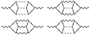
Figure 1: Representative four-loop diagrams for classes that might involve non-trivial $\gamma_{5}$ contributions. Wavy, dashed and straight lines represent gauge bosons, scalar bosons and fermions respectively.

In the literature one finds various prescriptions for the treatment of $\gamma_{5}$ in $D$ dimensions, see, e.g., Refs. tHooft:1972tcz ; Korner:1991sx ; Larin:1993tq ; Jegerlehner:2000dz ; Zerf:2019ynn . Many of these have been successfully applied in various calculations either in pure QCD or at lower loop order. In our opinion there is no practical prescription that can be applied at fourth order in perturbation theory. However, very recently in Ref. Poole:2019txl ; Poole:2019kcm Weyl consistency conditions Osborn:1989td ; Jack:1990eb ; Osborn:1991gm ; Jack:2013sha have been used in order to establish, with the help of “Osborn’s equation”, relations between coefficients of the general four-loop gauge, three-loop Yukawa and two-loop scalar beta function. It was realized in Poole:2019txl ; Poole:2019kcm that these relations fix all non-trivial $\gamma_{5}$ contributions to the four-loop gauge coupling beta function in terms of known coefficients of the three-loop Yukawa beta function. In particular, the results of Poole:2019txl ; Poole:2019kcm could resolve the ambiguity of the four-loop top Yukawa contribution to the beta function of the strong coupling constant, identified in Bednyakov:2015ooa ; Zoller:2015tha .

This observation fixes the outline for our computation; we decompose the beta functions into colour structures of the three gauge groups. We then perform an explicit computation of those parts of the renormalization constants that do not involve traces with an odd number of $\gamma_{5}$ matrices and fix the remaining parts using the results obtained in Poole:2019txl ; Poole:2019kcm . In addition, in Refs. Poole:2019txl ; Poole:2019kcm many further relations have been established that demonstrate the consistency between predictions derived from Osborn’s equation and explicit computations.

Calculation. For the computation of the gauge coupling renormalization constants, one can, in principle, use any vertex that contains the respective coupling at tree level. The renormalization constant is then obtained by

$$Z_{g_{i}} = \frac{Z_{\rm vert}}{\Pi_{k}\sqrt{Z_{k,{\rm wf}}}}\,,$$ (8)

where $Z_{\rm vert}$ stands for the renormalization constant of the vertex and $Z_{k,{\rm wf}}$ for the wave function renormalization constants ($k$ runs over all external particles). For the $\mathrm{SU}(2)$ and $\mathrm{SU}(3)$ gauge groups, it is advantageous to choose the ghost–gauge-boson vertices since one has to deal with fewer diagrams, amounting to ${\cal O}(350,000)$ for $\mathrm{SU}(2)$ and ${\cal O}(200,000)$ for $\mathrm{SU}(3)$ at four-loop order. For the $\mathrm{U}(1)$ gauge group, it is sufficient to consider the gauge boson propagator renormalization constant for which ${\cal O}(200,000)$ four-loop diagrams have to be computed. Sample Feynman diagrams for the various Green’s functions we consider are shown in Fig. 2.

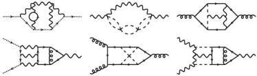
Figure 2: Sample Feynman diagrams contributing to the Green’s functions that have been used for our calculation of the gauge coupling renormalization constants. Solid, dashed, dotted, curly and wavy lines denote fermions, scalar bosons, ghosts, gluons and electroweak gauge bosons respectively.

Our calculation is based on a well-tested setup, which uses qgraf Nogueira:1991ex for the generation of the amplitudes and q2e and exp Harlander:1997zb ; Seidensticker:1999bb ; q2eexp for the mapping to integral families and generation of FORM Ruijl:2017dtg code. We use color vanRitbergen:1998pn for the computation of the $\mathrm{SU}(2)$ and $\mathrm{SU}(3)$ colour factors. Before the computation we combine diagrams with the same colour structure and integral family to form so-called “superdiagrams”, which guarantees possible cancellations at earlier stages of the calculation. This reduces the computational effort required.

In the unbroken phase of the SM, all particles are massless, and thus all two-point Green’s functions lead to massless propagator-type integrals up to four loops. Furthermore, one may set one of the external momenta of the three-point Green’s functions to zero. This is possible since the diagrams are logarithmically divergent, and thus the ultra-violet divergences, which must be computed to obtain the renormalization constants in the $\overline{\rm MS}$ scheme, are independent of kinematic quantities. Consequently, one only needs to compute massless propagator-type integrals up to four loops; this also holds for vertex corrections. For this task we use the program FORCER Ruijl:2017cxj .

In our calculation we use an anti-commuting $\gamma_{5}$, with $\gamma_{5}^{2}=1$, and set traces with an odd number of $\gamma_{5}$ occurrences to zero. These contributions to the beta functions (and thus to the gauge coupling renormalization constants) are reconstructed using the approach described in the previous section. Note that the ghost–gauge-boson vertices do not suffer from ambiguities related to $\gamma_{5}$. This allows us to reconstruct the non-trivial $\gamma_{5}$ contributions to the renormalization constants of the gauge boson wave-functions.

We retain full dependence on all three gauge parameters during the calculation. Whereas the renormalization constants for the vertices and wave functions still depend on the gauge parameters, the dependence drops out in the renormalization constants of the gauge couplings. This serves as a welcome check of our calculation.

As a further strong check we use the triple gauge boson vertices for the $\mathrm{SU}(2)$ and $\mathrm{SU}(3)$ gauge bosons to re-compute the gauge coupling renormalization constants, and find agreement. Furthermore, we verify by explicit calculation that $\mathrm{U}(1)$ loop corrections to the triple gauge boson vertex vanish after all bare Feynman diagrams are added. The calculation of these Green’s functions are significantly more costly than our default choice; for this reason we fix the gauge parameters to the Feynman gauge for these Green’s functions only.

We have performed several cross-checks of our four-loop expressions with results available in the literature. The pure gauge-fermion parts of $\beta_{2}$ and $\beta_{3}$ agree with the findings for a general Yang-Mills theory with fermions in the fundamental representation vanRitbergen:1997va ; Czakon:2004bu . Furthermore, the contributions to $\beta_{3}$ involving only the strong gauge coupling, the top quark Yukawa coupling and the quartic scalar coupling agree with Bednyakov:2015ooa ; Zoller:2015tha .

Finally, the Weyl consistency conditions from Refs. Poole:2019txl ; Poole:2019kcm represent powerful cross-checks on various coefficients in the beta functions, via their relation to the general result. The parametrization of the general four-loop gauge beta function (valid for all renormalizable four-dimensional quantum field theories) has 202 coefficients. As mentioned above, the four calculated in Poole:2019txl determine all contributions from traces over an odd number of $\gamma_{5}$ matrices, and are used directly in the computation of the beta functions. While we do not yet have a complete determination of the other 198, matching the general result to our SM calculation does uniquely fix 80; comparison with the full set of 261 consistency conditions in Poole:2019kcm (which also involve coefficients of the general three-loop Yukawa beta function) verifies these 80, and fixes another 28. Crucially, we find that these 108 coefficients (and by extension our four-loop computation) are indeed consistent with all Weyl consistency conditions, providing highly non-trivial corroboration.

Results. Our final results for the gauge coupling beta functions contain the full dependence on the gauge and Higgs self couplings and the third generation Yukawa couplings. The analytic results are available in computer-readable from progdata . Due to space restrictions we reproduce below the results for vanishing bottom and tau Yukawa couplings, $\alpha_{5}=\alpha_{6}=0$, and for numerical values of the $\mathrm{SU}(2)$ and $\mathrm{SU}(3)$ Casimir invariants. They are given by

$$\beta_{1}=\frac{\alpha^{2}_{1}}{\left(4\pi\right)^{2}}\left(\frac{82}{5}\right)+\frac{\alpha^{2}_{1}}{\left(4\pi\right)^{3}}\left(\frac{398\alpha_{1}}{25}+\frac{54\alpha_{2}}{5}+\frac{176\alpha_{3}}{5}-\frac{34\alpha_{4}}{5}\right)+\frac{\alpha^{2}_{1}}{\left(4\pi\right)^{4}}\bigg{(}-\frac{388613\alpha_{1}^{2}}{6000}+\frac{123\alpha_{1}\alpha_{2}}{40}-\frac{548\alpha_{1}\alpha_{3}}{75}$$

$$\vphantom{\bigg{[}}+\frac{789\alpha_{2}^{2}}{16}-\frac{12\alpha_{2}\alpha_{3}}{5}+\frac{1188\alpha_{3}^{2}}{5}-\frac{2827\alpha_{1}\alpha_{4}}{200}-\frac{471\alpha_{2}\alpha_{4}}{8}-\frac{116\alpha_{3}\alpha_{4}}{5}+\frac{189\alpha_{4}^{2}}{4}+\frac{54\alpha_{1}\alpha_{7}}{25}+\frac{18\alpha_{2}\alpha_{7}}{5}-\frac{36\alpha_{7}^{2}}{5}\bigg{)}$$

$$\vphantom{\bigg{[}}+\frac{\alpha^{2}_{1}}{\left(4\pi\right)^{5}}\bigg{[}-\alpha_{1}^{3}\left(\frac{143035709}{1080000}+\frac{1638851\zeta_{3}}{5625}\right)-\alpha_{1}^{2}\alpha_{2}\left(\frac{3819731}{24000}-\frac{16529\zeta_{3}}{125}\right)-\alpha_{1}^{2}\alpha_{3}\left(\frac{3629273}{6750}-\frac{720304\zeta_{3}}{1125}\right)$$

$$\vphantom{\bigg{[}}+\alpha_{1}\alpha_{2}^{2}\left(\frac{572059}{14400}-\frac{6751\zeta_{3}}{75}\right)-\frac{69\alpha_{1}\alpha_{2}\alpha_{3}}{25}+\alpha_{1}\alpha_{3}^{2}\left(\frac{333556}{675}-\frac{274624\zeta_{3}}{225}\right)-\alpha_{2}^{3}\left(\frac{117923}{2880}+\frac{3109\zeta_{3}}{5}\right)$$

$$\vphantom{\bigg{[}}-\alpha_{2}^{2}\alpha_{3}\left(\frac{41971}{90}-\frac{7472\zeta_{3}}{15}\right)-\alpha_{2}\alpha_{3}^{2}\left(\frac{1748}{3}-\frac{2944\zeta_{3}}{5}\right)+\alpha_{3}^{3}\left(\frac{6116}{15}-\frac{18560\zeta_{3}}{9}\right)+\alpha_{1}^{2}\alpha_{4}\left(\frac{8978897}{72000}+\frac{2598\zeta_{3}}{125}\right)$$

$$\vphantom{\bigg{[}}-\alpha_{1}\alpha_{2}\alpha_{4}\left(\frac{42841}{800}+\frac{1122\zeta_{3}}{25}\right)-\alpha_{1}\alpha_{3}\alpha_{4}\left(\frac{2012}{75}-\frac{408\zeta_{3}}{25}\right)-\alpha_{2}^{2}\alpha_{4}\left(\frac{439841}{960}-\frac{616\zeta_{3}}{5}\right)+\alpha_{2}\alpha_{3}\alpha_{4}\left(\frac{1468}{5}-\frac{1896\zeta_{3}}{5}\right)$$

$$\vphantom{\bigg{[}}-\alpha_{3}^{2}\alpha_{4}\left(\frac{11462}{45}-\frac{3184\zeta_{3}}{5}\right)+\alpha_{1}\alpha_{4}^{2}\left(\frac{29059}{160}-\frac{357\zeta_{3}}{25}\right)+\alpha_{2}\alpha_{4}^{2}\left(\frac{71463}{160}+\frac{639\zeta_{3}}{5}\right)+\alpha_{3}\alpha_{4}^{2}\left(\frac{1429}{5}-240\zeta_{3}\right)$$

$$\vphantom{\bigg{[}}-\alpha_{4}^{3}\left(\frac{13653}{40}+\frac{102\zeta_{3}}{5}\right)+\frac{3627\alpha_{1}^{2}\alpha_{7}}{500}+\frac{1917\alpha_{1}\alpha_{2}\alpha_{7}}{50}+\frac{889\alpha_{2}^{2}\alpha_{7}}{20}-\frac{1926\alpha_{1}\alpha_{4}\alpha_{7}}{25}-\frac{162\alpha_{2}\alpha_{4}\alpha_{7}}{5}-\frac{474\alpha_{4}^{2}\alpha_{7}}{5}$$

$$\vphantom{\bigg{[}}-\frac{1269\alpha_{1}\alpha_{7}^{2}}{25}-\frac{981\alpha_{2}\alpha_{7}^{2}}{5}+\frac{1188\alpha_{4}\alpha_{7}^{2}}{5}+\frac{624\alpha_{7}^{3}}{5}\bigg{]}~{},$$ (9)

$$\beta_{2}=\frac{\alpha^{2}_{2}}{\left(4\pi\right)^{2}}\left(-\frac{38}{3}\right)+\frac{\alpha^{2}_{2}}{\left(4\pi\right)^{3}}\left(\frac{18\alpha_{1}}{5}+\frac{70\alpha_{2}}{3}+48\alpha_{3}-6\alpha_{4}\right)+\frac{\alpha^{2}_{2}}{\left(4\pi\right)^{4}}\bigg{(}-\frac{5597\alpha_{1}^{2}}{400}+\frac{873\alpha_{1}\alpha_{2}}{40}-\frac{4\alpha_{1}\alpha_{3}}{5}$$

$$\vphantom{\bigg{[}}+\frac{324953\alpha_{2}^{2}}{432}+156\alpha_{2}\alpha_{3}+324\alpha_{3}^{2}-\frac{593\alpha_{1}\alpha_{4}}{40}-\frac{729\alpha_{2}\alpha_{4}}{8}-28\alpha_{3}\alpha_{4}+\frac{147\alpha_{4}^{2}}{4}+\frac{6\alpha_{1}\alpha_{7}}{5}+6\alpha_{2}\alpha_{7}-12\alpha_{7}^{2}\bigg{)}$$

$$\vphantom{\bigg{[}}+\frac{\alpha^{2}_{2}}{\left(4\pi\right)^{5}}\bigg{[}-\alpha_{1}^{3}\left(\frac{6418229}{72000}-\frac{21173\zeta_{3}}{375}\right)-\alpha_{1}^{2}\alpha_{2}\left(\frac{787709}{4800}-\frac{659\zeta_{3}}{25}\right)-\alpha_{1}^{2}\alpha_{3}\left(\frac{52297}{450}-\frac{2032\zeta_{3}}{15}\right)+\frac{161\alpha_{1}\alpha_{2}\alpha_{3}}{5}$$

$$\vphantom{\bigg{[}}-\alpha_{1}\alpha_{2}^{2}\left(\frac{375767}{2880}-\frac{4631\zeta_{3}}{15}\right)-\alpha_{1}\alpha_{3}^{2}\left(\frac{1748}{9}-\frac{2944\zeta_{3}}{15}\right)+\alpha_{2}^{3}\left(\frac{124660945}{15552}-\frac{78803\zeta_{3}}{9}\right)-\alpha_{2}^{2}\alpha_{3}\left(\frac{72881}{18}-\frac{16432\zeta_{3}}{3}\right)$$

$$\vphantom{\bigg{[}}+\alpha_{2}\alpha_{3}^{2}\left(\frac{10348}{3}-2560\zeta_{3}\right)+\alpha_{3}^{3}\left(\frac{1028}{3}-\frac{7040\zeta_{3}}{3}\right)+\alpha_{1}^{2}\alpha_{4}\left(\frac{465089}{4800}-\frac{498\zeta_{3}}{25}\right)-\alpha_{1}\alpha_{2}\alpha_{4}\left(\frac{102497}{480}+28\zeta_{3}\right)$$

$$\vphantom{\bigg{[}}+\alpha_{1}\alpha_{3}\alpha_{4}\left(\frac{796}{15}-\frac{376\zeta_{3}}{5}\right)-\alpha_{2}^{2}\alpha_{4}\left(\frac{500665}{576}-\frac{478\zeta_{3}}{3}\right)-\alpha_{2}\alpha_{3}\alpha_{4}\left(\frac{1444}{3}+56\zeta_{3}\right)-\alpha_{3}^{2}\alpha_{4}\left(\frac{614}{3}-336\zeta_{3}\right)$$

$$\vphantom{\bigg{[}}+\alpha_{1}\alpha_{4}^{2}\left(\frac{3161}{32}+\frac{153\zeta_{3}}{5}\right)+\alpha_{2}\alpha_{4}^{2}\left(\frac{30213}{32}-63\zeta_{3}\right)+\alpha_{3}\alpha_{4}^{2}\left(239-144\zeta_{3}\right)-\alpha_{4}^{3}\left(\frac{2143}{8}+18\zeta_{3}\right)+\frac{457\alpha_{1}^{2}\alpha_{7}}{100}$$

$$\vphantom{\bigg{[}}+\frac{69\alpha_{1}\alpha_{2}\alpha_{7}}{2}+\frac{2905\alpha_{2}^{2}\alpha_{7}}{12}-\frac{54\alpha_{1}\alpha_{4}\alpha_{7}}{5}-150\alpha_{2}\alpha_{4}\alpha_{7}-78\alpha_{4}^{2}\alpha_{7}-\frac{327\alpha_{1}\alpha_{7}^{2}}{5}-363\alpha_{2}\alpha_{7}^{2}+300\alpha_{4}\alpha_{7}^{2}+208\alpha_{7}^{3}\bigg{]}\,,$$ (10)

$$\beta_{3}=\frac{\alpha^{2}_{3}}{\left(4\pi\right)^{2}}\left(-28\right)+\frac{\alpha^{2}_{3}}{\left(4\pi\right)^{3}}\left(\frac{22\alpha_{1}}{5}+18\alpha_{2}-104\alpha_{3}-8\alpha_{4}\right)+\frac{\alpha^{2}_{3}}{\left(4\pi\right)^{4}}\bigg{(}-\frac{523\alpha_{1}^{2}}{30}-\frac{3\alpha_{1}\alpha_{2}}{10}+\frac{109\alpha_{2}^{2}}{2}+\frac{308\alpha_{1}\alpha_{3}}{15}$$

$$\vphantom{\bigg{[}}+84\alpha_{2}\alpha_{3}+130\alpha_{3}^{2}-\frac{101\alpha_{1}\alpha_{4}}{10}-\frac{93\alpha_{2}\alpha_{4}}{2}-160\alpha_{3}\alpha_{4}+60\alpha_{4}^{2}\bigg{)}$$

$$\vphantom{\bigg{[}}+\frac{\alpha^{2}_{3}}{\left(4\pi\right)^{5}}\bigg{[}-\alpha_{1}^{3}\left(\frac{6085099}{54000}-\frac{17473\zeta_{3}}{225}\right)-\alpha_{1}^{2}\alpha_{2}\left(\frac{46951}{1200}-\frac{973\zeta_{3}}{25}\right)-\alpha_{1}^{2}\alpha_{3}\left(\frac{35542}{135}-\frac{902\zeta_{3}}{9}\right)+\frac{69\alpha_{1}\alpha_{2}\alpha_{3}}{5}$$

$$\vphantom{\bigg{[}}-\alpha_{1}\alpha_{2}^{2}\left(\frac{37597}{720}-\frac{691\zeta_{3}}{15}\right)-\alpha_{1}\alpha_{3}^{2}\left(\frac{57739}{135}-\frac{32476\zeta_{3}}{45}\right)-\alpha_{2}^{3}\left(\frac{176815}{432}+935\zeta_{3}\right)+\alpha_{2}^{2}\alpha_{3}\left(\frac{3812}{9}-\frac{950\zeta_{3}}{3}\right)$$

$$\vphantom{\bigg{[}}-\alpha_{2}\alpha_{3}^{2}\left(\frac{5969}{3}-3476\zeta_{3}\right)+\alpha_{3}^{3}\left(\frac{127118}{9}-\frac{179792\zeta_{3}}{9}\right)+\alpha_{1}^{2}\alpha_{4}\left(\frac{362287}{3600}-\frac{19\zeta_{3}}{25}\right)+\alpha_{1}\alpha_{2}\alpha_{4}\left(\frac{77}{40}-54\zeta_{3}\right)$$

$$\vphantom{\bigg{[}}-\alpha_{1}\alpha_{3}\alpha_{4}\left(\frac{1283}{15}+\frac{32\zeta_{3}}{5}\right)-\alpha_{2}^{2}\alpha_{4}\left(\frac{12887}{48}-117\zeta_{3}\right)-\alpha_{2}\alpha_{3}\alpha_{4}\left(473+288\zeta_{3}\right)-\alpha_{3}^{2}\alpha_{4}\left(\frac{26836}{9}-1088\zeta_{3}\right)$$

$$\vphantom{\bigg{[}}+\alpha_{1}\alpha_{4}^{2}\left(\frac{3641}{40}+\frac{42\zeta_{3}}{5}\right)+\alpha_{2}\alpha_{4}^{2}\left(\frac{3201}{8}+90\zeta_{3}\right)+\alpha_{3}\alpha_{4}^{2}\left(1708-384\zeta_{3}\right)-\alpha_{4}^{3}\left(423+24\zeta_{3}\right)-120\alpha_{4}^{2}\alpha_{7}+144\alpha_{4}\alpha_{7}^{2}\bigg{]}\,,$$ (11)

where $\zeta_{3}$ is the Riemann zeta function evaluated at argument 3. It has been observed in Bednyakov:2015ooa ; Zoller:2015tha that at four-loop order the top quark Yukawa corrections amount to 7% of the corrections to $\beta_{3}$. It is interesting to note that the remaining terms, computed in this letter, cancel much of this contribution such that at the scale $\mu=M_{Z}$, about 99% of the four-loop coefficient is provided by the pure QCD contribution. At three loops this is not the case; here the remaining terms cancel about 40% of the pure QCD contribution and thus have a significant effect on the value. For this reason, the complete four-loop contribution to $\beta_{3}$ provides a large correction compared to the three-loop contributions. We find that the four-loop contributions to $\beta_{1}$, $\beta_{2}$ and $\beta_{3}$ amount to 8%, 5% and 127% of the three-loop contributions.

Summary. We compute analytic expressions for the four-loop gauge coupling beta functions in the SM, which require a consistent treatment of $\gamma_{5}$ in $D=4-2\epsilon$ space-time dimensions. We circumvent this problem by exploiting the findings of Refs. Poole:2019txl ; Poole:2019kcm , which fix the relevant terms through relations with known, unambiguous, lower-order results. Our calculation neglects the Yukawa contributions from the first and second generations, which are numerically small; their inclusion would not pose any practical problem. The calculation performed in this letter represents the highest full-SM loop calculation of phenomenologically relevant quantities to date.

Acknowledgements. This research was supported by the Deutsche Forschungsgemeinschaft (DFG, German Research Foundation) under grant 396021762 — TRR 257 “Particle Physics Phenomenology after the Higgs Discovery” and AET is partially supported by the Danish National Research Foundation under grant DNRF:90. FH acknowledges the support of the DFG-funded Doctoral School KSETA. CP thanks $\text{CP}^{3}$-Origins, where most of his contributions to this project were carried out under grant DNRF:90.

References

- (1) F. Bezrukov, M. Y. Kalmykov, B. A. Kniehl and M. Shaposhnikov, JHEP 1210 (2012) 140 [arXiv:1205.2893 [hep-ph]].
- (2) G. Degrassi, S. Di Vita, J. Elias-Miro, J. R. Espinosa, G. F. Giudice, G. Isidori and A. Strumia, JHEP 1208 (2012) 098 [arXiv:1205.6497 [hep-ph]].
- (3) S. Alekhin, A. Djouadi and S. Moch, Phys. Lett. B 716 (2012) 214 [arXiv:1207.0980 [hep-ph]].
- (4) E. Bagnaschi, G. Degrassi, S. Paßehr and P. Slavich, Eur. Phys. J. C 79 (2019) no.11, 910 [arXiv:1908.01670 [hep-ph]].
- (5) D. J. Gross and F. Wilczek, Phys. Rev. Lett. 30 (1973) 1343.
- (6) H. D. Politzer, Phys. Rev. Lett. 30 (1973) 1346.
- (7) D. R. T. Jones, Nucl. Phys. B 75 (1974) 531.
- (8) W. E. Caswell, Phys. Rev. Lett. 33, 244 (1974).
- (9) O. V. Tarasov and A. A. Vladimirov, Sov. J. Nucl. Phys. 25 (1977) 585 [Yad. Fiz. 25 (1977) 1104].
- (10) E. Egorian and O. V. Tarasov, Teor. Mat. Fiz. 41 (1979) 26 [Theor. Math. Phys. 41 (1979) 863].
- (11) O. V. Tarasov, A. A. Vladimirov and A. Y. Zharkov, Phys. Lett. 93B, 429 (1980).
- (12) S. A. Larin and J. A. M. Vermaseren, Phys. Lett. B 303 (1993) 334 [hep-ph/9302208].
- (13) T. van Ritbergen, J. A. M. Vermaseren and S. A. Larin, Phys. Lett. B 400 (1997) 379 [hep-ph/9701390].
- (14) M. Czakon, Nucl. Phys. B 710 (2005) 485 [hep-ph/0411261].
- (15) P. A. Baikov, K. G. Chetyrkin and J. H. Kühn, Phys. Rev. Lett. 118 (2017) no.8, 082002 [arXiv:1606.08659 [hep-ph]].
- (16) F. Herzog, B. Ruijl, T. Ueda, J. A. M. Vermaseren and A. Vogt, JHEP 1702 (2017) 090 [arXiv:1701.01404 [hep-ph]].
- (17) T. Luthe, A. Maier, P. Marquard and Y. Schroder, JHEP 1710 (2017) 166 [arXiv:1709.07718 [hep-ph]].
- (18) D. R. T. Jones, Phys. Rev. D 25 (1982) 581.
- (19) M. E. Machacek and M. T. Vaughn, Nucl. Phys. B 222 (1983) 83.
- (20) M. E. Machacek and M. T. Vaughn, Nucl. Phys. B 236 (1984) 221.
- (21) M. E. Machacek and M. T. Vaughn, Nucl. Phys. B 249 (1985) 70.
- (22) L. N. Mihaila, J. Salomon and M. Steinhauser, Phys. Rev. Lett. 108 (2012) 151602 [arXiv:1201.5868 [hep-ph]].
- (23) L. N. Mihaila, J. Salomon and M. Steinhauser, Phys. Rev. D 86 (2012) 096008 [arXiv:1208.3357 [hep-ph]].
- (24) A. V. Bednyakov, A. F. Pikelner and V. N. Velizhanin, JHEP 1301 (2013) 017 [arXiv:1210.6873 [hep-ph]].
- (25) K. G. Chetyrkin and M. F. Zoller, JHEP 1206 (2012) 033 [arXiv:1205.2892 [hep-ph]].
- (26) A. V. Bednyakov, A. F. Pikelner and V. N. Velizhanin, Phys. Lett. B 722 (2013) 336 [arXiv:1212.6829 [hep-ph]].
- (27) A. V. Bednyakov, A. F. Pikelner and V. N. Velizhanin, Phys. Lett. B 737 (2014) 129 [arXiv:1406.7171 [hep-ph]].
- (28) F. Herren, L. Mihaila and M. Steinhauser, Phys. Rev. D 97 (2018) no.1, 015016 [arXiv:1712.06614 [hep-ph]].
- (29) K. G. Chetyrkin and M. F. Zoller, JHEP 1304 (2013) 091 Erratum: [JHEP 1309 (2013) 155] [arXiv:1303.2890 [hep-ph]].
- (30) A. V. Bednyakov, A. F. Pikelner and V. N. Velizhanin, Nucl. Phys. B 875 (2013) 552 [arXiv:1303.4364 [hep-ph]].
- (31) A. V. Bednyakov, A. F. Pikelner and V. N. Velizhanin, Nucl. Phys. B 879 (2014) 256 [arXiv:1310.3806 [hep-ph]].
- (32) S. P. Martin, Phys. Rev. D 92 (2015) no.5, 054029 [arXiv:1508.00912 [hep-ph]].
- (33) K. G. Chetyrkin and M. F. Zoller, JHEP 1606 (2016) 175 [arXiv:1604.00853 [hep-ph]].
- (34) A. V. Bednyakov and A. F. Pikelner, Phys. Lett. B 762 (2016) 151 [arXiv:1508.02680 [hep-ph]].
- (35) M. F. Zoller, JHEP 1602 (2016) 095 [arXiv:1508.03624 [hep-ph]].
- (36) G. ’t Hooft and M. J. G. Veltman, Nucl. Phys. B 44 (1972) 189.
- (37) J. G. Korner, D. Kreimer and K. Schilcher, Z. Phys. C 54 (1992) 503.
- (38) S. A. Larin, Phys. Lett. B 303 (1993) 113 [hep-ph/9302240].
- (39) F. Jegerlehner, Eur. Phys. J. C 18 (2001) 673 [hep-th/0005255].
- (40) N. Zerf, arXiv:1911.06345 [hep-ph].
- (41) C. Poole and A. E. Thomsen, Phys. Rev. Lett. 123 (2019) no.4, 041602 [arXiv:1901.02749 [hep-th]].
- (42) C. Poole and A. E. Thomsen, JHEP 1909 (2019) 055 [arXiv:1906.04625 [hep-th]].
- (43) H. Osborn, Phys. Lett. B 222 (1989) 97.
- (44) I. Jack and H. Osborn, Nucl. Phys. B 343 (1990) 647.
- (45) H. Osborn, Nucl. Phys. B 363 (1991) 486.
- (46) I. Jack and H. Osborn, Nucl. Phys. B 883 (2014) 425 [arXiv:1312.0428 [hep-th]].
- (47) P. Nogueira, J. Comput. Phys. 105 (1993) 279.
- (48) R. Harlander, T. Seidensticker and M. Steinhauser, Phys. Lett. B 426 (1998) 125 [hep-ph/9712228].
- (49) T. Seidensticker, hep-ph/9905298.
-
(50)
http://sfb-tr9.ttp.kit.edu/software/html/q2eexp.html. - (51) B. Ruijl, T. Ueda and J. Vermaseren, arXiv:1707.06453 [hep-ph].
- (52) T. van Ritbergen, A. N. Schellekens and J. A. M. Vermaseren, Int. J. Mod. Phys. A 14 (1999) 41 [hep-ph/9802376].
- (53) B. Ruijl, T. Ueda and J. A. M. Vermaseren, arXiv:1704.06650 [hep-ph].
-
(54)
https://www.ttp.kit.edu/preprints/2019/ttp19-047/.