Alternative physics to understand wall turbulence:
Navier–Stokes equations with modified linear dynamics

Abstract

Despite the nonlinear nature of wall turbulence, there is evidence that the energy-injection mechanisms sustaining wall turbulence can be ascribed to linear processes. The different scenarios stem from linear stability theory and comprise exponential instabilities from mean-flow inflection points, transient growth from non-normal operators, and parametric instabilities from temporal mean-flow variations, among others. These mechanisms, each potentially capable of leading to the observed turbulence structure, are rooted in simplified theories and conceptual arguments. Whether the flow follows any or a combination of them remains unclear. In the present study, we devise a collection of numerical experiments in which the Navier-Stokes equations are sensibly modified to quantify the role of the different linear mechanisms. This is achieved by direct numerical simulation of turbulent channel flows with constrained energy extraction from the streamwise-averaged mean-flow. We demonstrate that (i) transient growth alone is not sufficient to sustain wall turbulence and (ii) the flow remains turbulent when the exponential instabilities are suppressed. On the other hand, we show that (iii) transient growth combined with the parametric instability of the time-varying mean-flow is able to sustain turbulence.

1 Introduction: linear theories of self-sustaining wall turbulence

Turbulence is a primary example of a highly nonlinear phenomenon. Nevertheless, there is ample agreement that the energy-injection mechanisms sustaining wall turbulence can be partially attributed to linear processes [1]. The different mechanisms have their origins in linear stability theory [2, 3, 4, 5, 6, 7, 8] and constitute the foundations of many control and modeling strategies [9, 10]. Despite the ubiquity of linear theories, the significance of different instabilities in fully developed turbulence remains outstanding, and its relevance is consequential to comprehend, model, and control the structure of wall-bounded turbulence by linear methods (e.g., Refs. [11, 6, 7, 12]). Here, we devise a collection of numerical experiments of turbulent flows over a flat wall in which the Navier–Stokes equations are minimally altered to suppress the energy transfer from the mean flow to the fluctuating velocities via different linear instabilities.

Several linear mechanisms have been proposed within the fluid mechanics community as plausible scenarios to rationalize the transfer of energy from the large-scale mean flow to the fluctuating velocities. Generally, it is agreed that the ubiquitous streamwise rolls (regions of rotating fluid) and streaks (regions of low and high streamwise velocity with respect to the mean) [13, 14] are involved in a quasi-periodic regeneration cycle [15, 16, 17, 18, 19, 20] and that their space-time structure plays a crucial role in sustaining shear-driven turbulence (e.g., Refs. [21, 22, 23, 3, 4, 5, 24, 18, 25, 26, 27]). Accordingly, the flow is often decomposed into two components: a base flow defined by some averaging procedure over the instantaneous flow, and the three-dimensional fluctuations (or perturbations) about that base flow. In this manner, the ultimate cause maintaining turbulence is conceptualized as the energy transfer from the base flow to the fluctuating flow. Various base flows have been proposed in the literature depending on the number of flow directions and period of time to average the instantaneous flow. Here, we select as base flow the instantaneous streamwise-averaged velocity $U(y,z,t)$ with zero wall-normal ($V=0$) and spanwise ($W=0$) flow, where $y$ and $z$ are the wall-normal and spanwise directions. Figure 1 illustrates this flow decomposition.

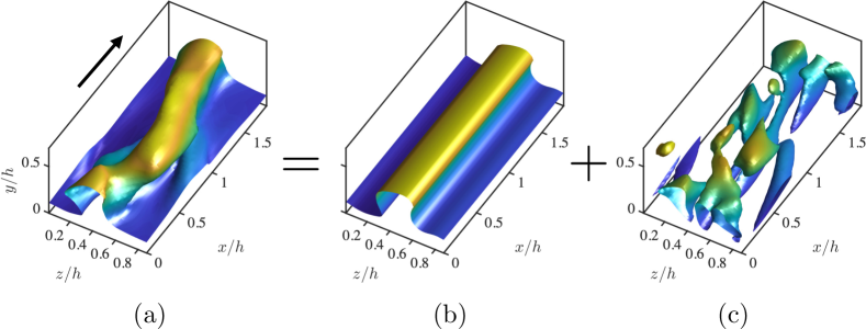
Figure 1: Decomposition of the instantaneous flow into a streamwise mean base flow and fluctuations. Instantaneous isosurface of streamwise velocity for (a) the total flow $u$, (b) the streak base flow $U$, and (c) the absolute value of the fluctuations $|u^{\prime}|$. The values of the isosurfaces are 0.8 (a and b) and 0.1 (c) of the maximum streamwise velocity. Colors represent the distance to the wall located at $y=0$. The arrow in panel (a) indicates the mean flow direction.

The linear mechanisms proposed to explain the energy transfer from the mean to the fluctuating flow can be categorized into: (i) modal inflectional instability of the mean streamwise flow, (ii) non-modal transient growth, and (iii) non-modal transient growth assisted by parametric instability of the time-varying mean streamwise flow.

In mechanism (i), it is hypothesized that the energy is transferred from the mean profile $U(y,z,t)$ to the fluctuating flow through a modal inflectional instability in the form of strong spanwise flow variations [3, 4], corrugated vortex sheets [28], or intense localized patches of low-momentum fluid [29, 30]. Inasmuch as the instantaneous realizations of the streaky flow are strongly inflectional, the flow $U(y,z,t)$ is invariably unstable at a frozen time $t$ [27]. These inflectional instabilities are markedly robust and their excitation has been proposed to be the mechanism that replenishes the perturbation energy of the turbulent flow [3, 4, 29, 28, 31, 30]. Consequently, the exponential instability of the streak is thought to be central to the maintenance of wall turbulence.

Mechanism (ii), transient growth, involves the redistribution of fluid near the wall by streamwise vortices leading to the formation of streaks via the Orr/lift-up mechanism [32, 33, 23, 34, 18]. In this case, the mean flow, while exponentially stable, supports the growth of perturbations for a period of time due to the non-normality of the linear operator that governs the evolution of fluctuations. This process is referred to as non-modal transient growth (e.g., Refs. [23, 6, 35, 36]). Additional studies suggest that the generation of streaks is due to the structure-forming properties of the linearized Navier–Stokes operator, independent of any organized vortices [37], but the non-modal transient growth is still invoked. The transient growth scenario gained even more popularity since the work by Schoppa & Hussain [5] (see also Ref. [38]), who argued that transient growth may be the most relevant mechanism not only for streak formation but also for their eventual breakdown. Schoppa & Hussain [5] showed that most streaks detected in actual wall-turbulence simulations are indeed exponentially stable. Instead, the loss of stability of the streaks is better explained by transient growth of perturbations that leads to vorticity sheet formation and nonlinear saturation.

Finally, mechanism (iii) has been proposed in recent years by Farrell, Ioannou and coworkers [24, 26]. They adopted the perspective of statistical state dynamics (SSD) to develop a tractable theory for the maintenance of wall turbulence. Within the SSD framework, the perturbations are maintained by an essentially time-dependent, parametric, non-normal interaction of the fluctuations and the streak, rather than by the inflectional instability of the streaky flow discussed above (see also Ref. [39]).

The scenarios (i), (ii), and (iii), although consistent with the observed turbulence structure [19], are rooted in simplified theoretical arguments. Whether the flow follows these or any other combination of mechanisms for maintaining the turbulent fluctuations is still to be established. In this study, we evaluate the contribution of each linear mechanism by direct numerical simulation of channel flows with constrained energy extraction from the mean flow.

The study is organized as follows: Section 2 contains the numerical details of the simulations. The results are presented in Section 3, which is further subdivided into three subsections each devoted to the investigation of one linear mechanism. Finally, conclusions and future directions are offered in Section 4.

2 Numerical experiments of minimal channel units

To investigate the role of different linear mechanisms, we examine data from spatially and temporally resolved simulations of an incompressible turbulent channel flow driven by a constant mean pressure gradient. Hereafter, the streamwise, wall-normal, and spanwise directions of the channel are denoted by $x$, $y$, and $z$, respectively, and the corresponding flow velocity components and pressure by $u$, $v$, $w$, and $p$. The density of the fluid is $\rho$ and the channel height is $h$. The wall is located at $y=0$, where no-slip boundary conditions apply, whereas free stress and no penetration conditions are imposed at $y=h$. The streamwise and spanwise directions are periodic. The grid resolution of the simulations in $x$, $y$, and $z$ is $64\times 90\times 64$, respectively, which is fine enough to resolve all the scales of the fluid motion.

The simulations are characterized by the non-dimensional Reynolds number, defined as the ratio between the largest and the smallest length-scales of the flow, $h$ and $\delta_{v}=\nu/u_{\tau}$, respectively, where $\nu$ is the kinematic viscosity of the fluid and $u_{\tau}$ is the characteristic velocity based on the friction at the wall [40]. The Reynolds number selected is $\mathrm{Re}_{\tau}=\delta/\delta_{v}\approx 180$, which provides a sustained turbulent flow at an affordable computational cost [41]. In all cases, the flow is simulated for at least $100h/u_{\tau}$ units of time, which is orders of magnitude longer than the typical lifetime of individual energy-containing eddies [42]. The streamwise, wall-normal, and spanwise sizes of the computational domain are $L_{x}^{+}\approx 337$, $L_{y}^{+}\approx 186$, and $L_{z}^{+}\approx 168$, respectively, where the superscript $+$ denotes quantities normalized by $\nu$ and $u_{\tau}$. Jimenez & Moin [22] showed that turbulence in such domains contains an elementary flow unit comprised of a single streamwise streak and a pair of staggered quasi-streamwise vortices, that reproduce the dynamics of the flow in larger domains. Hence, the current numerical experiment provides a fundamental testbed for studying the self-sustaining cycle of wall turbulence.

The simulations are performed with a staggered, second-order, finite differences scheme [43] and a fractional-step method [44] with a third-order Runge-Kutta time-advancing scheme [45]. The solution is advanced in time using a constant time step such that the Courant–Friedrichs–Lewy condition is below 0.5. The code has been presented in previous studies on turbulent channel flows [46, 47, 48]. The streamwise and spanwise resolutions are $\Delta x^{+}\approx 6.5$ and $\Delta z^{+}\approx 3.3$, respectively, and the minimum and maximum wall-normal resolutions are $\Delta y_{\mathrm{min}}^{+}\approx 0.2$ and $\Delta y_{\mathrm{max}}^{+}\approx 6.1$. All the simulations were run for at least $100h/u_{\tau}$ after transients.

We focus on the dynamics of the fluctuating velocities $\bm{u}^{\prime}\equiv(u^{\prime},v^{\prime},w^{\prime})$, defined with respect to the streak base flow

$$U(y,z,t)\equiv\frac{1}{L_{x}}\int_{0}^{L_{x}}u(x,y,z,t)\,\mathrm{d}x,$$ (1)

such that $u^{\prime}\equiv u-U$, $v^{\prime}\equiv v$, and $w^{\prime}\equiv w$. We have not included in the base flow the contributions from the streamwise average $w$ and $w$ components, as is traditionally done in the study of stability of the streaky flow [49, 4, 5]. The fluctuating velocity vector $\bm{u}^{\prime}\equiv(u^{\prime},v^{\prime},w^{\prime})$ is governed by

$$\frac{\partial\bm{u}^{\prime}}{\partial t}=\mathcal{L}(U)\bm{u}^{\prime}+\bm{N}(\bm{u}^{\prime}),$$ (2)

where $\mathcal{L}$ is the linearized Navier–Stokes operator for the fluctuating state vector about the instantaneous $U(y,z,t)$ (see Figure 1b) and $\bm{N}$ collectively denotes the nonlinear terms (which are quadratic with respect to fluctuating flow fields). Both $\mathcal{L}$ and $\bm{N}$ account for the kinematic divergence-free condition $\bm{\nabla}\cdot\bm{u}^{\prime}=0$. The corresponding equation of motion for $U(y,z,t)$ is obtained by averaging the Navier–Stokes equations in the streamwise direction.

We consider three numerical experiments. First, we simulate the Navier–Stokes equations without any modification, in which the linear instabilities of perturbations are naturally allowed. We refer to this case as the “regular channel”. The two additional experiments entail a modification of the Navier–Stokes equations and they are described in the sections below.

3 Wall turbulence with constrained linear mechanisms

3.1 Wall turbulence without exponential instability of the streaks

The exponential instabilities of the instantaneous streamwise mean flow at a given time are obtained by eigenanalysis of the matrix representation of the operator $\mathcal{L}$ about the instantaneous base flow $U$,

$$\mathcal{L}(U)=\mathcal{Q}\Lambda\mathcal{Q}^{-1},$$ (3)

where $\mathcal{Q}$ consists of the eigenvectors organized in columns and $\Lambda$ is the diagonal matrix of associated eigenvalues, $\lambda_{j}+i\omega_{j}$. The base flow is unstable when any of the growth rates $\lambda_{j}$ is positive. Figure 2 shows a representative example of the streamwise velocity of an unstable eigenmode. The predominant eigenmode has the typical sinuous structure of positive and negative patches of velocity flanking the velocity streak side by side, which may lead to its subsequent meandering and breakdown.

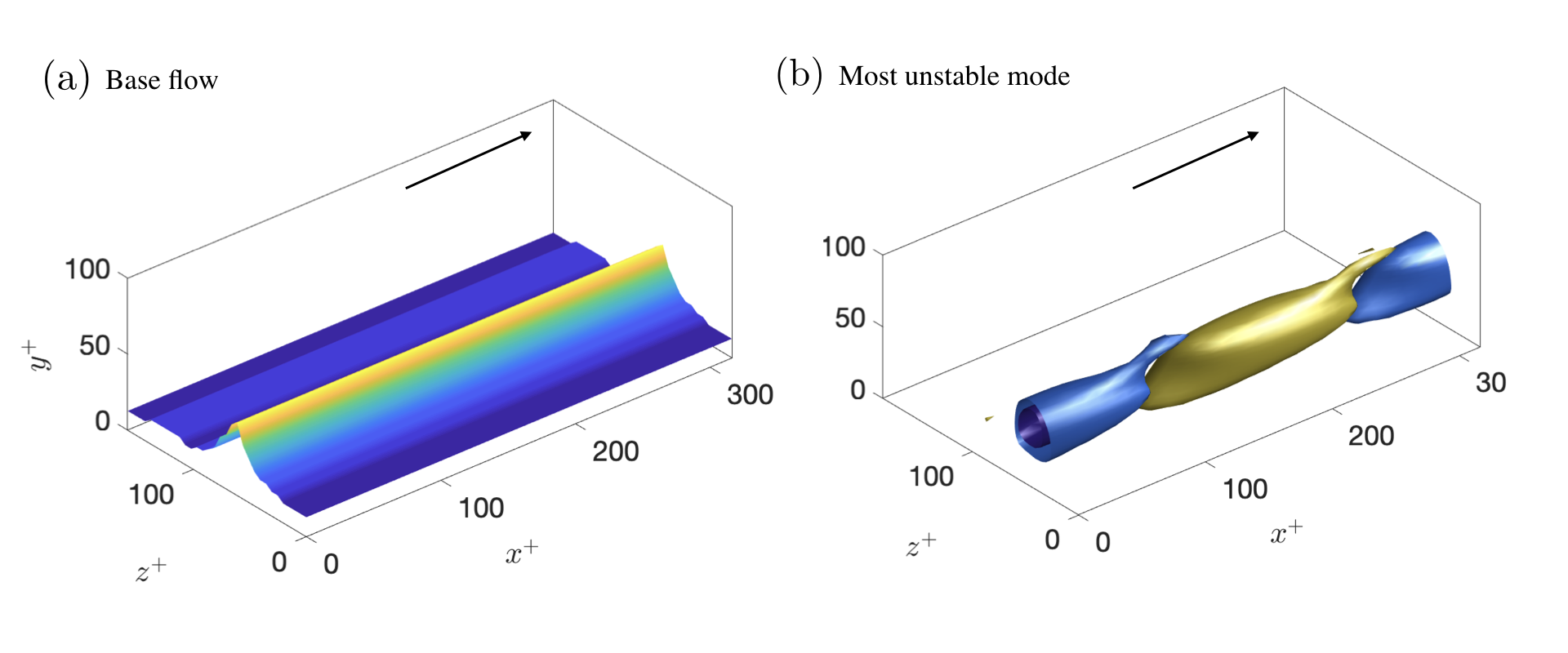
Figure 2: Representative exponential instability of the streak. (a) Instantaneous isosurface of the base flow $U$. The value of the isosurface is $0.8$ of the maximum. (b) Isosurface of the instantaneous streamwise velocity for the eigenmode associated with the most unstable eigenvalue $\lambda_{\mathrm{max}}h/u_{\tau}\approx 3$ at $t=5.1h/u_{\tau}$. The values of the isosurface are $-0.5$ (blue) and $0.5$ (yellow) of the maximum streamwise velocity.

Figure 3 shows the probability density functions of the growth rate of the four least stable eigenvalues of $\mathcal{L}(U)$. On average, the operator $\mathcal{L}$ contains 2 to 3 unstable eigenmodes at any given instant. The time-history of the maximum growth rate supported by $\mathcal{L}$, denoted by $\lambda_{\mathrm{max}}$, is shown in Figure 4(a). The flow is exponentially unstable ($\lambda_{\mathrm{max}}>0$) 70% of the time. The corresponding kinetic energy of the perturbations averaged over the channel is shown in Figure 4(b).

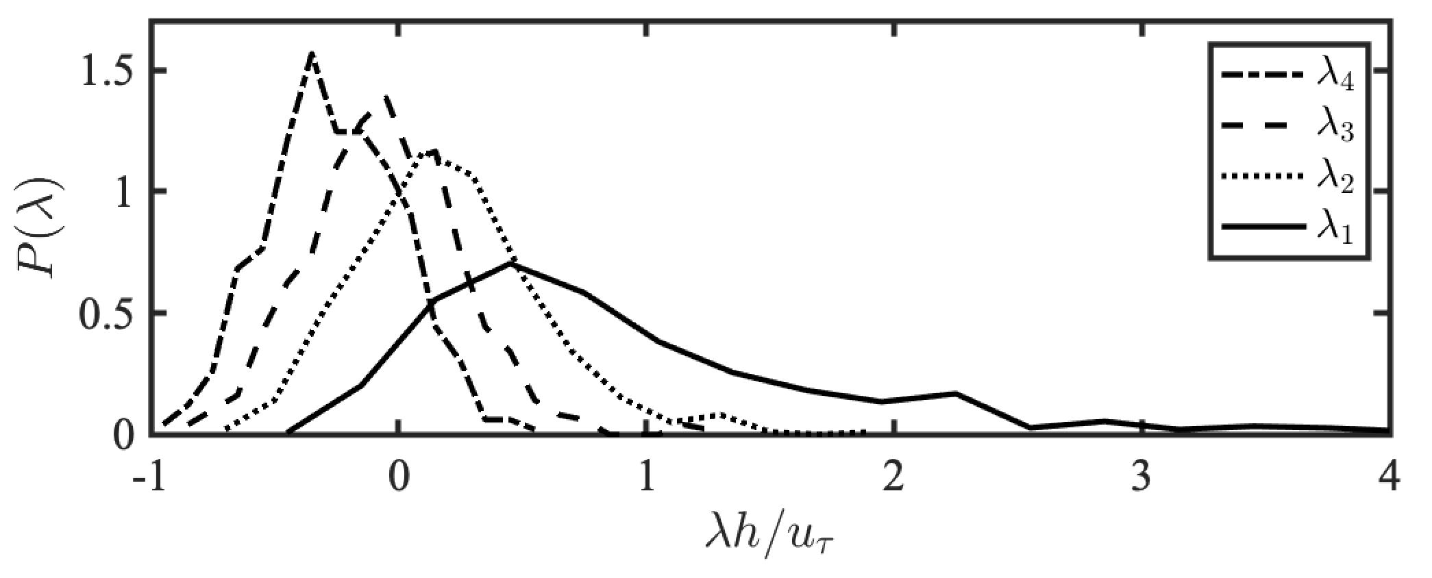
Figure 3: Probability density functions of the growth rate of the four least stable eigenvalues of $\mathcal{L}(U)$, $\lambda_{1}>\lambda_{2}>\lambda_{3}>\lambda_{4}$.

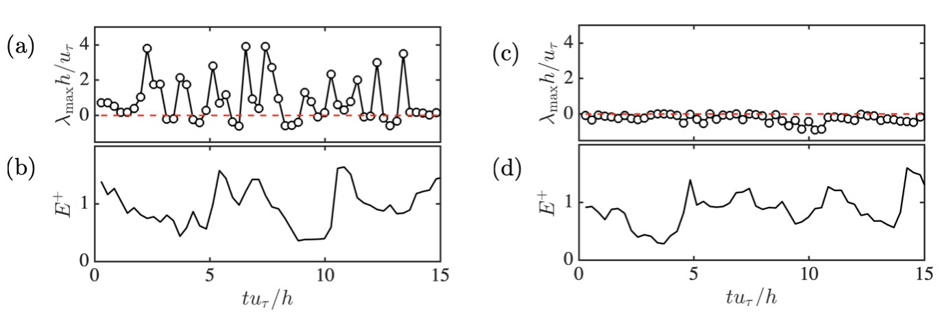
Figure 4: (a,c) The time-history of the most unstable eigenvalue $\lambda_{\rm max}$ of (a) $\mathcal{L}$ for the regular channel flow and (c) $\tilde{\mathcal{L}}$ for the channel flow with suppressed exponential instabilities. (b,d) The time-history of the kinetic energy of the perturbations $E=\bm{u}^{\prime}\cdot\bm{u}^{\prime}/2$ averaged over the channel domain for (b) the regular channel flow and (d) for the channel flow with suppressed exponential instabilities.

Rigorously, we expect the linear instability to manifest in the flow only when $\lambda_{\mathrm{max}}$ is much larger than time rate of change of $U$, defined as $\lambda_{U}\equiv(\mathrm{d}E_{U}/\mathrm{d}t)/(2E_{U})$ with $E_{U}\equiv 1/(L_{y}L_{z})\int_{0}^{L_{y}}\int_{0}^{L_{z}}(1/2)U^{2}\,\mathrm{d}y\mathrm{d}z$ the streak energy. The ratio $\lambda_{\mathrm{max}}/\lambda_{U}$ for $\lambda_{\mathrm{max}}>0$ is on average around $10$, i.e., the time-changes of the streak $U$ are ten times slower than the maximum growth rate predicted by the linear stability analysis. Hence, the exponential growth of disturbances is supported for a non-negligible fraction of the flow history, and exponential instabilities stand as a potential mechanism sustaining wall turbulence. Note that the argument above does not imply that exponential instabilities are necessarily relevant for the flow, but only that they could be realizable in terms of characteristic time-scales.

For the second numerical experiment, we modify the operator $\mathcal{L}$ so that all the unstable eigenmodes are rendered neutral for all times. We refer to this case as the “channel with suppressed exponential instabilities” and we inquire whether turbulence is sustained in this case. The approach is implemented by replacing $\mathcal{L}$ at each time-instance by the exponentially-stable operator

$$\tilde{\mathcal{L}}=\mathcal{Q}\tilde{\Lambda}\mathcal{Q}^{-1},$$ (4)

where $\tilde{\Lambda}$ is the stabilized version of $\Lambda$ obtained by setting the real part of all unstable eigenvalues of $\Lambda$ equal to zero. We do not modify the equation of motion for $U(y,z,t)$. The stable counterpart of $\mathcal{L}$ in Eq. (4), $\tilde{\mathcal{L}}$, represents the smallest intrusion into the system to achieve exponentially stable wall turbulence at all times while leaving other linear mechanisms almost intact (we discuss this further in Section 3.2). Figure 4(c) shows the maximum modal growth rate of $\tilde{\mathcal{L}}$ at selected times with the instabilities successfully neutralized. It was verified that turbulence persists when $\mathcal{L}$ is replaced by $\tilde{\mathcal{L}}$ (Figure 4d).

The main result of this section is presented in Figure 5, which compares the mean velocity profiles and turbulence intensities for the regular channel and the channel with suppressed exponential instabilities. The statistics are compiled for the statistical steady state after any initial transients. Notably, the turbulent channel flow without exponential instabilities is capable of sustaining turbulence. The difference of roughly 15%–25% in the turbulence intensities between the cases indicates that, even if the linear instability of the streak manifests in the flow, it is not a requisite for maintaining turbulent fluctuations. The new flow equilibrates at a state with augmented streamwise fluctuations (Figure 5b) and depleted cross flow (Figure 5c,d). The outcome is consistent with the occasional inhibition of the streak meandering or breakdown via exponential instability, which enhances the streamwise velocity fluctuations, whereas wall-normal and spanwise turbulence intensities are diminished due to a lack of vortices succeeding the collapse of the streak.

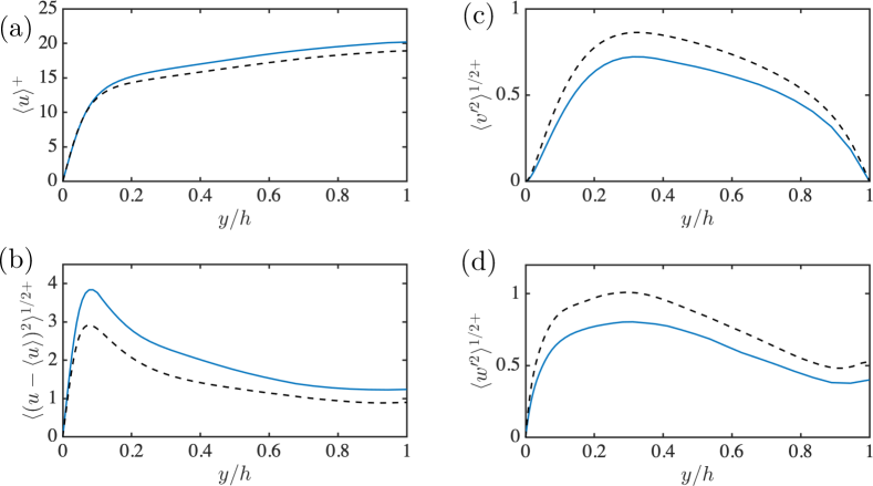
Figure 5: (a) Streamwise mean velocity profile as a function of the wall-normal distance and (b) streamwise, (c) wall-normal, and (d) spanwise root-mean-squared fluctuating velocities for the regular channel (            ) and the channel with suppressed exponential instabilities (   ). The Reynolds number of both simulations is $\mathrm{Re}_{\tau}=186$. Angle brackets represent averaging in the homogeneous directions and time.

3.2 Wall turbulence exclusively supported by transient growth

We quantify the transient growth supported by $U(y,z,t_{0})$ at a fixed time $t_{0}$ as the mechanism energizing the fluctuating velocities. The potential effectiveness of transient growth is characterized by the optimal gain, $G$, defined as

$$G(t=T)=\frac{\bm{u}^{\prime\dagger}\exp(\mathcal{L}^{\dagger}T)\exp(\mathcal{L}T)\bm{u}^{\prime}}{\bm{u}^{\prime\dagger}\bm{u}^{\prime}},$$ (5)

where $(\cdot)^{\dagger}$ denotes conjugate transpose, and $T$ is the time-horizon for optimal gain. The square of the largest singular value of the linear propagator

$$\exp(\mathcal{L}T)=\mathcal{M}\Sigma\mathcal{N}^{\dagger},$$ (6)

provides the maximum gain, $G_{\mathrm{max}}$, where the columns of $\mathcal{M}$ and of $\mathcal{N}$ are the input modes (or left-singular vectors) and output modes (or right-singular vectors) of $\exp(\mathcal{L}T)$, respectively, and $\Sigma$ is a diagonal matrix, whose entries are the singular values of $\exp(\mathcal{L}T)$ denoted by $\sigma_{j}$ [23, 50].

Figure 6 provides a visual representation of the input and output modes associated with the maximum optimal gain for one selected instant. The example displays a backwards-leaning perturbation (input mode) tilted forward by the mean shear (output mode). The process is reminiscent of the linear Orr/lift-up mechanism driven by continuity and the wall-normal transport of momentum characteristic of the bursting process and streak formation [51, 52, 34, 1].

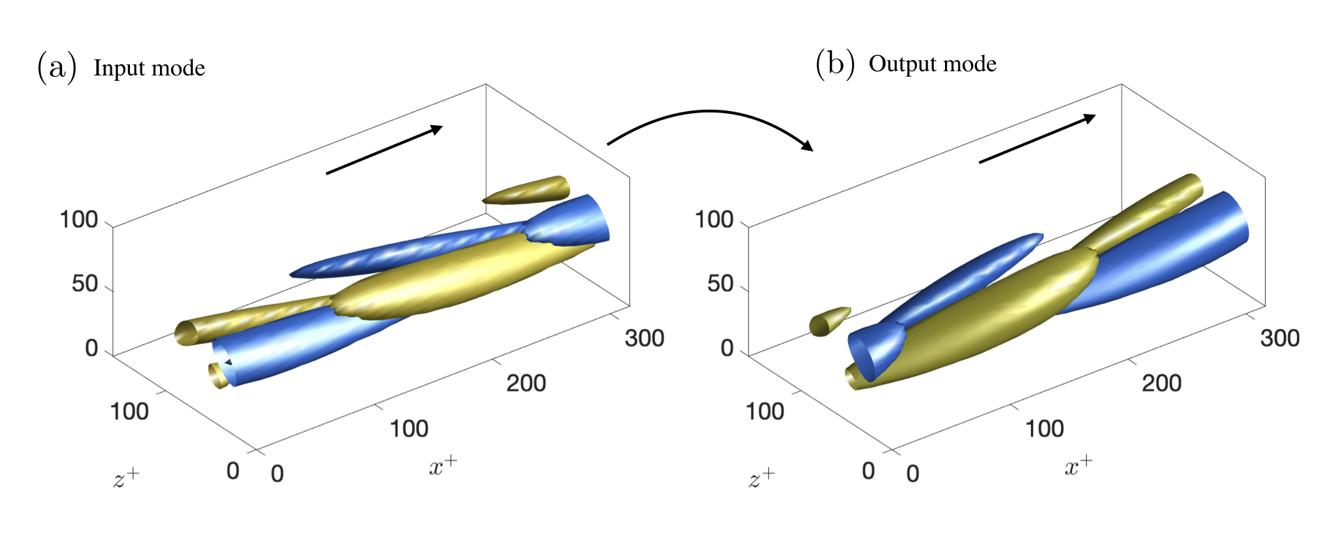
Figure 6: Representative input and output modes associated with transient growth of the streak. Isosurfaces of (a) the input and (b) the output wall-normal velocity mode associated with the largest singular value of $\mathcal{L}(U)$ at $t=5h/u_{\tau}$. The isosurface are $-0.5$ (blue) and $0.5$ (yellow) of the maximum wall-normal velocity. The gain is $G_{\mathrm{max}}=110$. The result is for the regular channel.

The maximum optimal gain for $T=0.5h/u_{\tau}$ is included in Figure 7 as a function of the reference time $t_{0}$. The results are for the channel with suppressed exponential instabilities, which are on average 10% lower than the maximum optimal gains for the regular channel (as discussed below). The gain attains amplification values of the input mode of the order of 100. Therefore, transient growth supported by the “frozen” mean streamwise flow $U$ stands as a tenable candidate to sustain wall turbulence. It is worth noting that the gains $G_{\mathrm{max}}$ due to the non-normality of an instantaneous mean flow with spanwise/crosstream structure $U(y,z,t)$ are remarkably large. This is in contrast with the gains traditionally reported for the mean velocity profile defined as the average streamwise velocity in all homogeneous directions and time, for which $G_{\mathrm{max}}$ is limited to a more modest factor of 10 [6, 53].

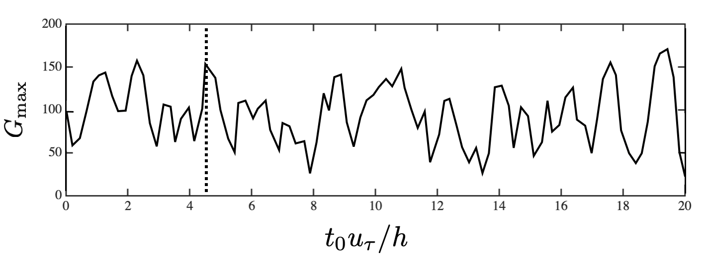
Figure 7: Maximum optimal gain ($G_{\mathrm{max}}$) supported by $U(y,z,t_{0})$ as a function of the fixed time $t_{0}$ and for a time horizon $T=0.5u_{\tau}/h$. The results are for the channel with suppressed exponential instabilities. The vertical dashed line represents the time selected for Fig. 8.

The effect of non-modal transient growth as a main source for energy injection to the fluctuating velocities is assessed by “freezing” the base flow $U(y,z,t_{0})$ at the instant $t_{0}$. In order to steer clear of the effect of exponential instabilities, the numerical experiment is performed for the channel with suppressed exponential instabilities. Simulations are then continued for $t>t_{0}$. This procedure was repeated for 100 different $t_{0}$. The set-up disposes of energy transfers that are due to both modal and parametric instabilities, while maintaining the transient growth of perturbations. The expected scenario consistent with sustained turbulence [5] is the non-modal amplification of perturbations until saturation followed by nonlinear scattering and generation of new disturbances.

The evolution of the root-mean-squared fluctuating velocities for one of the experiments is shown in Figure 8, which contains instances from $t=t_{0}$ to $t=t_{0}+10h/u_{\tau}$. The particular $t_{0}$ selected is highlighted in Figure 7 and corresponds to a gain of $\sim$150. After freezing the base flow, turbulence decays and reaches a quasi-laminar state with residual turbulence intensities required to support the prescribed $U(y,z,t_{0})$. This behavior was observed for all of the one hundred cases investigated. Although not shown here, another hundred additional cases were investigated again by fixing $U(y,z,t_{0})$, but initializing the flow field with random perturbations, rather than utilizing as initial condition the already-existing fluctuating velocities at $t=t_{0}$. The intensities of the random perturbations were adjusted to be 10% higher than their values in the regular channel. All the additional simulations decayed similarly to the cases reported above. Consequently, our results suggest that turbulence is not exclusively supported by transient growth, at least when the magnitude of the perturbations corresponds to those typically encountered at the low Reynolds number used here. The outcome of this experiment does not imply that transient growth is inconsequential for wall turbulence, but merely that additional linear ingredients are needed to attain fully self-sustaining turbulence.

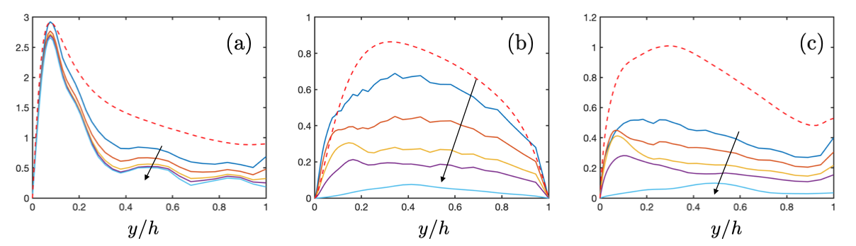
Figure 8: Turbulent channel exclusively supported by transient growth. Root-mean-squared (a) streamwise, (b) wall-normal, and (c) spanwise fluctuating velocities. The dashed line is for the regular channel and solid lines represent different times of a turbulent channel exclusively supported by transient growth from $t=t_{0}$ to $t=t_{0}+10h/u_{\tau}$, where $t_{0}$ is the instant at which the mean flow is frozen in time. The arrow indicates the direction of time.

To finalize our analysis on transient growth, we discuss briefly the implications of stabilizing the eigenvalues of $\mathcal{L}$ as discussed in Section 3.1. Due to the non-normal nature of $\mathcal{L}$, the suppression of exponential instabilities by Eq. (4) inevitably entails the modification of the non-normal characteristics of the operator. The impact on the amount of transient growth supported by $\mathcal{L}$ is quantified in Figure 9, which shows the maximum gain of $\mathcal{L}$ and $\tilde{\mathcal{L}}$ for different time horizons $T$. The decrease in the maximum gain is about 15% for $T\approx 0.6h/u_{\tau}$, but negligible for $T<0.4h/u_{\tau}$. In a preliminary work [27], we had proposed to incorporate the linear friction $-\mu\bm{u}^{\prime}$ into Eq. (2) in an attempt to damp all the unstable eigenvalues of $\mathcal{L}$. The results in Ref. [27] showed that turbulence was not sustained for the values of $\mu$ necessary to stabilize $\mathcal{L}$. However, a detailed analysis of the impact of the linear damping on transient growth shows that the decrease in the gains of $\mathcal{L}$ due to the drag term $-\mu\bm{u}^{\prime}$ is proportional to $\exp(-2\mu T)$. Hence, values of $\mu$ necessary to neutralize the exponential instabilities of $\mathcal{L}$ are highly disruptive of the transient growth, which might be the cause for the lack of sustained turbulence in Ref. [27]. The maximum gain of $\mathcal{L}-\mu\mathcal{I}$, where $\mathcal{I}$ is the identity operator, is also included in Figure 9.

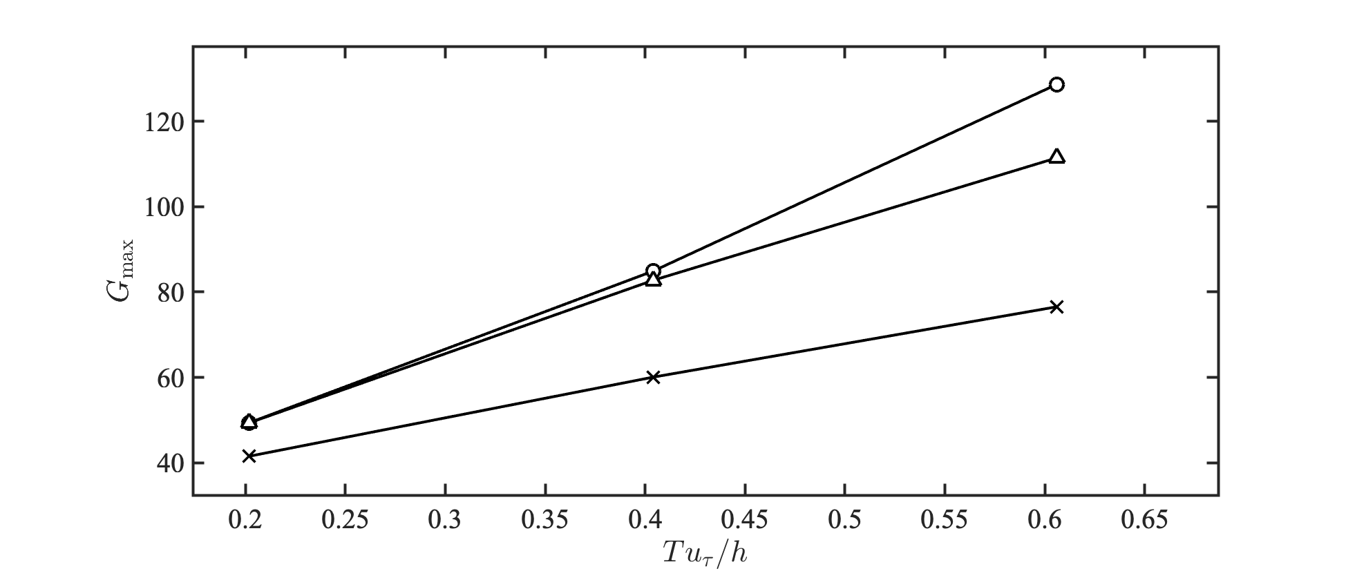
Figure 9: Maximum optimal gain, $G_{\mathrm{max}}$, attained at the time $t=T$ for the regular channel ($\circ$), channel with suppressed exponential instabilities ($\scriptstyle\triangle$), and channel with linear damping with $\mu=0.43u_{\tau}/h$ ($\times$).

3.3 The parametric instability: transient growth enhancement

The maintenance of turbulence by transient growth assisted by parametric instability was demonstrated in Section 3.1. Here, we review some aspects of the parametric amplification mechanisms by analyzing the results from the channel with suppressed exponential instabilities.

Parametric instability of the streak relies on an endogenous and essentially non-modal growth process that is inherent to time-dependent dynamical systems. The mechanism is analogous to the classic instability of a damped harmonic oscillator with periodically varying restoring force, in which the time-dependent variations of the eigenbasis has the potential to altering the instantaneous linear stability properties of the system. To clarify this process, let us reformulate the linear dynamics of Eq. (2) for a time period $T>0$ in terms of the propagator $\mathcal{P}_{t\rightarrow t+T}$ as

$$\bm{u}^{\prime}_{\mathrm{linear}}(t+T)=\mathcal{P}_{t\rightarrow t+T}\bm{u}^{\prime}(t).$$ (7)

The propagator $\mathcal{P}_{t\rightarrow t+T}$ represents the cumulative effect along the time $T$ of the linear operator $\tilde{\mathcal{L}}$. As such, it can be obtained by the discrete approximation under the assumption of small $\Delta t$ as

$$\mathcal{P}_{t\rightarrow t+T}\approx\exp\left[\tilde{\mathcal{L}}(t+n\Delta t)\Delta t\right]\dotsb\exp\left[\tilde{\mathcal{L}}(t+\Delta t)\Delta t\right]\exp\left[\tilde{\mathcal{L}}(t)\Delta t\right],$$ (8)

where $T=n\Delta t$, with $n$ a positive integer.

To evaluate the instabilities arising from the parametric mechanism, we reconstruct the propagator for the channel with suppressed exponential instabilities. A time-series of the base mean flow was stored and used to estimate $\mathcal{P}_{t\rightarrow t+T}$ following Eq. (8) with $T=h/u_{\tau}$. This estimation is then used to compute the largest singular value of $\mathcal{P}_{t\rightarrow t+T}$, which has a value equal to $\sigma_{\mathrm{max}}\approx 50$. The largest singular value $\sigma_{\mathrm{max}}$ can be compared to the non-parametric counterpart assuming a frozen mean flow

$$\mathcal{P}_{t\rightarrow t+T}^{0}=\exp\left[\tilde{\mathcal{L}}(t_{0})T\right],$$ (9)

which yields a value of $\sigma_{\mathrm{max}}^{0}\approx 10$. This result reveals the existence of enhanced growth rates owing to the time-variation of the streak reflected on $\tilde{\mathcal{L}}(t)$. Moreover, for $T\rightarrow\infty$, the growth rate of $\mathcal{P}_{t\rightarrow t+T}^{0}$ tends to $0$, as the operator $\tilde{\mathcal{L}}(t_{0})$ is exponentially stable. On the contrary, a time-varying $\tilde{\mathcal{L}}$ can produce finite exponential growth for an arbitrary $T$. It is here important to note that if the operators $\tilde{\mathcal{L}}(t)$ at each instance were also normal (additionally to being stable), parametric instability would not arise. This simple but revealing example illustrates how a time-dependent $U$ together with non-modal growth may provide the additional energy injection into the fluctuations to attain self-sustaining turbulence.

4 Conclusions

We have investigated the energy injection from the streamwise-averaged mean flow to the turbulent fluctuations. This energy transfer is believed to be correctly represented by the linearized Navier–Stokes equations, and three potential linear mechanisms have been considered, namely, exponential instability of the streamwise mean $U(y,z,t)$, non-modal transient growth, and non-modal transient growth supported by parametric instability.

We have devised two numerical experiments of a turbulent channel flow in which the linear operator is altered to neutralize one or various linear mechanisms for energy extraction. In the first experiment, the linear operator is modified to render any exponential instabilities of the streaks stable, thus precluding the energy transfer from the mean to the fluctuations via exponential growth. In the second experiment, we simulated turbulent channel flows with prescribed exponentially stable mean streamwise flow frozen in time, suppressing in that manner any potential parametric and exponential instabilities. Our results establish that wall turbulence with realistic mean velocity and turbulence intensities persists even when exponential instabilities are suppressed. On the contrary, turbulence decays when the energy transfer from the base flow to the fluctuating field occurs only via transient growth. These results argue in favor of the parametric-instability scenario proposed by Farrell, Ioannou, and co-workers as the basic mechanism sustaining wall turbulence [24, 26, 39].

Our conclusions are preliminary and refer to the dynamics of wall turbulence in channels computed using minimal flow units, chosen as simplified representations of naturally occurring wall turbulence. The approach presented in this study paves the path for future investigations at high-Reynolds-numbers turbulence obtained for larger unconstraining domains, in addition to extensions to different flow configurations in which the role of instabilities remains elusive.

References

References

- [1] J. Jiménez, “How linear is wall-bounded turbulence?,” Phys. Fluids, vol. 25, p. 110814, 2013.
- [2] W. C. Reynolds and A. K. M. F. Hussain, “The mechanics of an organized wave in turbulent shear flow. Part 3. Theoretical models and comparisons with experiments,” J. Fluid Mech., vol. 54, no. 2, pp. 263–288, 1972.
- [3] J. M. Hamilton, J. Kim, and F. Waleffe, “Regeneration mechanisms of near-wall turbulence structures,” J. Fluid Mech., vol. 287, pp. 317–348, 1995.
- [4] F. Waleffe, “On a self-sustaining process in shear flows,” Phys. Fluids, vol. 9, no. 4, pp. 883–900, 1997.
- [5] W. Schoppa and F. Hussain, “Coherent structure generation in near-wall turbulence,” J. Fluid Mech., vol. 453, pp. 57–108, 2002.
- [6] J. C. Del Álamo and J. Jiménez, “Linear energy amplification in turbulent channels,” J. Fluid Mech., vol. 559, pp. 205–213, 2006.
- [7] Y. Hwang and C. Cossu, “Linear non-normal energy amplification of harmonic and stochastic forcing in the turbulent channel flow,” J. Fluid Mech., vol. 664, pp. 51–73, 2010.
- [8] Y. Hwang and C. Cossu, “Self-sustained processes in the logarithmic layer of turbulent channel flows,” Phys. Fluids, vol. 23, no. 6, p. 061702, 2011.
- [9] J. Kim and T. R. Bewley, “A linear systems approach to flow control,” Annu. Rev. Fluid Mech., vol. 39, pp. 383–417, 12 2006.
- [10] P. Schmid and D. Henningson, Stability and Transition in Shear Flows. Applied Mathematical Sciences, Springer New York, 2012.
- [11] M. Högberg, T. R. Bewley, and D. S. Henningson, “Linear feedback control and estimation of transition in plane channel flow,” J. Fluid Mech., vol. 481, pp. 149–175, 2003.
- [12] P. Morra, O. Semeraro, D. S. Henningson, and C. Cossu, “On the relevance of Reynolds stresses in resolvent analyses of turbulent wall-bounded flows,” J. Fluid Mech., vol. 867, pp. 969–984, 2019.
- [13] P. S. Klebanoff, K. D. Tidstrom, and L. M. Sargent, “The three-dimensional nature of boundary-layer instability,” J. Fluid Mech., vol. 12, no. 1, pp. 1–34, 1962.
- [14] S. J. Kline, W. C. Reynolds, F. A. Schraub, and P. W. Runstadler, “The structure of turbulent boundary layers,” J. Fluid Mech., vol. 30, no. 4, pp. 741–773, 1967.
- [15] R. L. Panton, “Overview of the self-sustaining mechanisms of wall turbulence,” Prog. Aerosp. Sci., vol. 37, no. 4, pp. 341–383, 2001.
- [16] R. J. Adrian, “Hairpin vortex organization in wall turbulence,” Phys. Fluids, vol. 19, no. 4, p. 041301, 2007.
- [17] A. J. Smits, B. J. McKeon, and I. Marusic, “High-Reynolds number wall turbulence,” Annu. Rev. Fluid Mech., vol. 43, no. 1, pp. 353–375, 2011.
- [18] J. Jiménez, “Cascades in wall-bounded turbulence,” Annu. Rev. Fluid Mech., vol. 44, pp. 27–45, 2012.
- [19] J. Jiménez, “Coherent structures in wall-bounded turbulence,” J. Fluid Mech., vol. 842, p. P1, 2018.
- [20] A. Lozano-Durán, H. Bae, and M. Encinar, “Causality of energy-containing eddies in wall turbulence,” J. Fluid Mech., vol. 882, p. A2, 2019.
- [21] J. Kim, S. J. Kline, and W. C. Reynolds, “The production of turbulence near a smooth wall in a turbulent boundary layer,” J. Fluid Mech., vol. 50, pp. 133–160, 1971.
- [22] J. Jiménez and P. Moin, “The minimal flow unit in near-wall turbulence,” J. Fluid Mech., vol. 225, pp. 213–240, 4 1991.
- [23] K. M. Butler and B. F. Farrell, “Optimal perturbations and streak spacing in wall-bounded turbulent shear flow,” Phys. Fluids A, vol. 5, p. 774, 1993.
- [24] B. F. Farrell and P. J. Ioannou, “Dynamics of streamwise rolls and streaks in turbulent wall-bounded shear flow,” J. Fluid Mech., vol. 708, pp. 149–196, 2012.
- [25] N. C. Constantinou, A. Lozano-Durán, M.-A. Nikolaidis, B. F. Farrell, P. J. Ioannou, and J. Jiménez, “Turbulence in the highly restricted dynamics of a closure at second order: comparison with DNS,” J. Phys.: Conf. Series, vol. 506, p. 012004, apr 2014.
- [26] B. F. Farrell, P. J. Ioannou, J. Jiménez, N. C. Constantinou, A. Lozano-Durán, and M.-A. Nikolaidis, “A statistical state dynamics-based study of the structure and mechanism of large-scale motions in plane poiseuille flow,” J. Fluid Mech., vol. 809, pp. 290–315, 2016.
- [27] A. Lozano-Durán, M. Karp, and N. C. Constantinou, “Wall turbulence with constrained energy extraction from the mean flow,” Center for Turbulence Research - Annual Research Briefs, pp. 209–220, 2018.
- [28] G. Kawahara, J. Jiménez, M. Uhlmann, and A. Pinelli, “Linear instability of a corrugated vortex sheet – a model for streak instability,” J. Fluid Mech., vol. 483, pp. 315–342, 2003.
- [29] P. Andersson, L. Brandt, A. Bottaro, and D. S. Henningson, “On the breakdown of boundary layer streaks,” J. Fluid Mech., vol. 428, pp. 29–60, 2001.
- [30] M. J. P. Hack and P. Moin, “Coherent instability in wall-bounded shear,” J. Fluid Mech., vol. 844, pp. 917–955, 2018.
- [31] M. J. P. Hack and T. A. Zaki, “Streak instabilities in boundary layers beneath free-stream turbulence,” J. Fluid Mech., vol. 741, pp. 280–315, 2014.
- [32] M. T. Landahl, “Wave breakdown and turbulence,” SIAM J. Appl. Math, vol. 28, pp. 735–756, 1975.
- [33] B. F. Farrell and P. J. Ioannou, “Optimal excitation of three-dimensional perturbations in viscous constant shear flow,” Phys. Fluids, vol. 5, no. 6, pp. 1390–1400, 1993.
- [34] J. Kim and J. Lim, “A linear process in wall-bounded turbulent shear flows,” Phys. Fluids, vol. 12, no. 8, pp. 1885–1888, 2000.
- [35] P. J. Schmid, “Nonmodal stability theory,” Annu. Rev. Fluid Mech., vol. 39, no. 1, pp. 129–162, 2007.
- [36] C. Cossu, G. Pujals, and S. Depardon, “Optimal transient growth and very large–scale structures in turbulent boundary layers,” J. Fluid Mech., vol. 619, pp. 79–94, 2009.
- [37] S. I. Chernyshenko and M. F. Baig, “The mechanism of streak formation in near-wall turbulence,” J. Fluid Mech., vol. 544, pp. 99–131, 2005.
- [38] M. de Giovanetti, H. Sung, and Y. Hwang, “Streak instability in turbulent channel flow: the seeding mechanism of large-scale motions,” J. Fluid Mech., vol. 832, pp. 483–513, 2017.
- [39] B. F. Farrell, D. F. Gayme, and P. J. Ioannou, “A statistical state dynamics approach to wall turbulence,” Philos. Trans. Royal Soc. A, vol. 375, p. 20160081, 03 2017.
- [40] S. B. Pope, Turbulent Flows. Cambridge University Press, 2000.
- [41] J. Kim, P. Moin, and R. Moser, “Turbulence statistics in fully developed channel flow at low Reynolds number,” J. Fluid Mech., vol. 177, no. 1, pp. 133–166, 1987.
- [42] A. Lozano-Durán and J. Jiménez, “Time-resolved evolution of coherent structures in turbulent channels: characterization of eddies and cascades,” J. Fluid. Mech., vol. 759, pp. 432–471, 2014.
- [43] P. Orlandi, Fluid Flow Phenomena: A Numerical Toolkit. Fluid Flow Phenomena: A Numerical Toolkit, Springer, 2000.
- [44] J. Kim and P. Moin, “Application of a fractional-step method to incompressible Navier-Stokes equations,” J. Comp. Phys., vol. 59, pp. 308–323, 1985.
- [45] A. A. Wray, “Minimal-storage time advancement schemes for spectral methods,” tech. rep., NASA Ames Research Center, 1990.
- [46] A. Lozano-Durán and H. J. Bae, “Turbulent channel with slip boundaries as a benchmark for subgrid-scale models in LES,” Center for Turbulence Research - Annual Research Briefs, pp. 97–103, 2016.
- [47] H. J. Bae, A. Lozano-Durán, S. T. Bose, and P. Moin, “Turbulence intensities in large-eddy simulation of wall-bounded flows,” Phys. Rev. Fluids, vol. 3, p. 014610, Jan 2018.
- [48] H. J. Bae, A. Lozano-Durán, S. T. Bose, and P. Moin, “Dynamic slip wall model for large-eddy simulation,” J. Fluid Mech., vol. 859, pp. 400–432, 2019.
- [49] S. C. Reddy and D. S. Henningson, “Energy growth in viscous channel flows,” J. Fluid Mech., vol. 252, pp. 209–238, 1993.
- [50] B. F. Farrell and P. J. Ioannou, “Generalized Stability Theory. Part I: Autonomous Operators,” J. Atmos. Sci., vol. 53, no. 14, pp. 2025–2040, 1996.
- [51] W. M. Orr, “The stability or instability of the steady motions of a perfect liquid and of a viscous liquid. Part II: A viscous liquid,” Math. Proc. Royal Ir. Acad., vol. 27, pp. 69–138, 1907.
- [52] T. Ellingsen and E. Palm, “Stability of linear flow,” Phys. Fluids, vol. 18, no. 4, pp. 487–488, 1975.
- [53] G. Pujals, M. García-Villalba, C. Cossu, and S. Depardon, “A note on optimal transient growth in turbulent channel flows,” Phys. Fluids, vol. 21, no. 1, p. 015109, 2009.