Visualizing Planar and Space Implicit Real Algebraic Curves with Singularities^∗

CHEN Changbo^a,b $\cdot$ WU Wenyuan^a,b $\cdot$ FENG Yong^a,b Address: ^aChongqing Key Laboratory of Automated Reasoning and Cognition, Chongqing Institute of Green and Intelligent Technology, Chinese Academy of Sciences, Chongqing 400714, China
^bUniversity of Chinese Academy of Sciences, Beijing 100049, China
Email: chenchangbo@cigit.ac.cn, wuwenyuan@cigit.ac.cn, yongfeng@cigit.ac.cn ^∗This research was supported by NSFC (11771421, 11671377, 61572024), CAS “Light of West China” Program, cstc2018jcyj-yszxX0002 of Chongqing and the Key Research Program of Frontier Sciences of CAS (QYZDB-SSW-SYS026).

We present a new method for visualizing implicit real algebraic curves inside a bounding box in the $2$-D or $3$-D ambient space based on numerical continuation and critical point methods. The underlying techniques work also for tracing space curve in higher-dimensional space. Since the topology of a curve near a singular point of it is not numerically stable, we trace only the curve outside neighborhoods of singular points and replace each neighborhood simply by a point, which produces a polygonal approximation that is $\varepsilon$-close to the curve. Such an approximation is more stable for defining the numerical connectedness of the complement of the projection of the curve in $\mathbb{R}^{2}$, which is important for applications such as solving bi-parametric polynomial systems. The algorithm starts by computing three types of key points of the curve, namely the intersection of the curve with small spheres centered at singular points, regular critical points of every connected components of the curve, as well as intersection points of the curve with the given bounding box. It then traces the curve starting with and in the order of the above three types of points. This basic scheme is further enhanced by several optimizations, such as grouping singular points in natural clusters, tracing the curve by a try-and-resume strategy and handling “pseudo singular points”. The effectiveness of the algorithm is illustrated by numerous examples. This manuscript extends our preliminary results that appeared in CASC 2018.

Continuation method, critical point method, real algebraic curve, singularity

1 Introduction

Visualizing an implicit plane or space real algebraic curve is a classical and fundamental problem in computational geometry and computer graphics. There have been many works on this topic both in $2$-D [1, 2, 3, 4, 5, 6, 7, 8] and $3$-D [9, 10, 11] cases. In the literature, a correct visualization usually requires two conditions: $(i)$ the generated polygonal approximation is $\varepsilon$-close to the curve, and $(ii)$ the approximation is “topologically correct”, which often means that the approximation is isotopic to the curve. There are also many works [9, 12, 13, 14] focusing only on $(ii)$.

Different techniques [15, 16] exist for visualizing plane and space curves, such as implicit-to-parametric conversion, curve continuation and space subdivision. Symbolic or hybrid symbolic-numeric approaches stand out for being capable of computing the exact topology and many of them are variants of cylindrical algebraic decomposition. For continuation based approach, several difficulties arise, such as finding at least one seed point from each connected component, dealing with curve jumping and handling singularities. Each of the three problems has its own interests. For instance, there are several approaches for computing at least one witness points for a real variety, either symbolically [17, 18, 19] or numerically [20, 21, 22]. Different techniques for robustly tracing curves are proposed [23, 24, 25, 26, 21]. Techniques for handling singularities also exist [27, 28, 29].

For curves with singularities, observe that condition $(ii)$ is numerically ill-posed, since a slight perturbation may completely change the topology of the curve nearby a singular point, see Example 2.5 for instance. On the other hand, in many applications, such as solving bi-parametric polynomial systems, condition $(ii)$ is unnecessary. Let us illuminate this point now. For a given bi-parametric polynomial system, one can compute a border curve [30, 31], or a border polynomial [32] or discriminant variety [33] in general in the parametric space, where the complement of the curve is a disjoint union of connected open cells, such that above each cell the number of solutions of the system is constant and the solutions are continuous functions of parameters with disjoint graphs. Let $B$ be a border curve and $\mathaccent 869{B}$ be a polygonal approximation $\varepsilon$-close to it. In [30], we introduced the notion of $\varepsilon$-connectedness and showed that two points are $\varepsilon$-connected w.r.t. $\mathaccent 869{B}$ implies that they are connected w.r.t. $B$, which in turn implies that the parametric system has the same number of solutions at the two points. Thus an $\varepsilon$-approximation of the border curve meeting only condition $(i)$ is good enough for the purpose of solving parametric systems. The curve tracing subroutine in [30] relies on perturbation to handle singularities. In this work, we develop a perturbation free algorithm. The algorithm traces only the curve outside neighborhoods of singular points and replace each neighborhood simply by a point. Such produced approximation is more stable for defining the numerical connectedness of the complement of the curve than those approximations preserving the topology around singular points.

The paper is organized as follows. In Section 2, we formalize the problem and provide a theoretical base algorithm to guarantee $\varepsilon$-closeness based on a robust curve tracing method. Several strategies for improving the numerical stability of tracing is proposed in Section 3, such as tracing the curve away from the singular points rather than towards it, tracing the curve by a try-and-resume strategy, classifying singular points into natural clusters [34], and handling “pseudo singular points”. The theoretical algorithm may require the step size to be very small. In Section 4, we present a more practical algorithm based on optimizations in Section 3. Instead of preventing curve jumping, it maintains a simple data structure to detect curve jumping. The effectiveness of the algorithm is demonstrated through several nontrivial examples in Section 5. Finally, in Section 6, we draw the conclusion and point out some possible future directions to improve the current work. Compared with our CASC 2018 paper [35], our algorithm is now fully generalized to plot curve in $n$-dimensional ambient space. In particular, its effectiveness is demonstrated though visualizing space curves in $3$-D space in Section 5. Another new contribution of the paper is that we propose effective heuristic strategies to handle “pseudo singular points” in Section 3. Last but not least, we provide a proof of Theorem 2.4.

2 A theoretical base algorithm

It is highly nontrivial for continuation methods to guarantee that the polygonal chains are $\varepsilon$-close to the curve even when the curve contains no singular points. Robust tracing without curve jumping must be involved. In the literature, there are several techniques [23, 24, 25] that can solve this. Here we combine the technique of $\alpha$-theory [23, 24] with a technique developed in [21], which has been used to estimate the error of numerically computed border curve in [30]. In particular, we have Theorem 2.4, which provides a way to obtain $\varepsilon$-approximation of a regular section of a curve.

2.1 Preliminary

We first recall some well-known results which are important for the rest of the paper.

Throughout this paper, let $F=\{f_{1},\ldots,f_{n-1}\}\subseteq\mathbb{R}[x_{1},\ldots,x_{n}]$, $B\subset\mathbb{R}^{n}$ be a bounded box and $\varepsilon\in\mathbb{R}$ be a given precision. Let $\mathcal{J}_{F}$ be the Jacobian of $F$, or simply $\mathcal{J}$ if no confusion arises. We assume that $\mbox{{\rm dim}$(V_{\mathbb{C}}(F))$}=\mbox{{\rm dim}$(V_{\mathbb{R}}(F))$}=1$ and at almost all points of $V_{\mathbb{C}}(F)$, $\mathcal{J}$ has full rank $n-1$. Let $M_{i}$, $i=1,\ldots,{n}$, be respectively the submatrix of $\mathcal{J}$ by removing the $i$-th column of $\mathcal{J}$. Let $\Delta_{i}$, $i=1,\ldots,n$, be the determinant of $M_{i}$. Then the zero set of $F\cup\{\Delta_{1},\ldots,\Delta_{n}\}$ in $\mathbb{R}^{n}$ is the set of singular points of $V_{\mathbb{R}}(F)$, which is finite under our assumptions. Denote by ${\sf SingularPoints}(F,B)$ an operation which computes the set of singular points of $V_{\mathbb{R}}(F)$ inside $B$.

Let $W$ be a closed smooth component of $V_{\mathbb{R}}(F)$. Let $L:{a}{x}=d$ be a hyperplane in $\mathbb{R}^{n}$. Let ${x}^{*}$ be any point of $W$. The distance from $x^{*}$ to $L$ is given by $\displaystyle\delta({x}^{*})=\frac{|{a}{x}^{*}-d|}{\|{a}\|_{2}}$. By the method of Lagrange multipliers, the local extrema of the constrained optimization problem ${\rm min}~{}\delta({x})$ subject to $F({x})=0$ can be obtained by solving the system $G:=F\cup\{\mathcal{J}^{t}\lambda=a\}$, where $\lambda=(\lambda_{1},\ldots,\lambda_{n})$ are introduced new variables. Let $(x^{0},\lambda^{0})$ be a point of $V_{\mathbb{R}}(G)$ such that $\mathcal{J}_{F}$ has full rank at $x^{0}$, then by Proposition $2.2$ of [36], for almost all choices of $a$ in $\mathbb{R}^{n}$, $(x^{0},\lambda^{0})$ is an isolated point of $V_{\mathbb{R}}(G)$. Therefore, we can apply homotopy continuation method to find such isolated points. Denote by ${\sf WitnessPoints}(F,B)$ an operation which finds all such $x^{0}\in B$, denoted by $S$. If $x^{0}\in W$, $\mathcal{J}_{F}$ has full rank at $x^{0}$, thus $x^{0}\in S$. In other words, $S$ contains at least one point (called witness point) from each closed smooth component $W$ of $V_{\mathbb{R}}(F)$. Note that it is possible that $S$ may also contain witness points of non-closed components of $V_{\mathbb{R}}(F)$.

Let $\mathcal{J}(p)=U\Sigma V^{T}$ be the singular value decomposition (SVD) of $\mathcal{J}$ at a regular point $p$ of $V_{\mathbb{R}}(F)$, where $U$ and $V$ are orthogonal matrices of dimension $(n-1)\times(n-1)$ and $n\times n$ and $\Sigma={\rm diag}(\sigma_{1},\ldots,\sigma_{n-1})\in\mathbb{R}^{(n-1)\times n}$, where $\sigma_{1}>\cdots>\sigma_{n-1}>0$. The Eckhart-Young Theorem says that $\displaystyle\sigma_{i}=\underset{{\rm rank}(B)=i-1}{{\rm min}}\|\mathcal{J}-B\|_{2}$, $i=1,\ldots,n-1$. Therefore, the smallest singular value $\sigma_{n-1}$ measures the 2-norm distance of $\mathcal{J}$ to the set of all rank-deficient matrices. In other words, it tells how $\mathcal{J}$ is close to be singular.

Let $V=[v_{1}\mid\dots\mid v_{n}]$, where each $v_{i}$ is a column vector. By $\mathcal{J}(p)=U\Sigma V^{T}$, we have $\mathcal{J}(p)v_{n}=0$. That is $v_{n}$ is a tangent vector which can be chosen as the direction to trace the curve. We define an operator ${{t}}$ which computes $v_{n}$ from $\mathcal{J}(p)$, that is $v_{n}={{t}}(\mathcal{J}(p))$. More precisely, to trace the curve, we adopt a predictor-corrector method. In the predictor step, we choose a step size $h>0$ and compute the predictor point $q=p+hv_{n}$. In the corrector step, we apply Newton iterations $\displaystyle q_{i+1}=q_{i}-\bigg{(}\begin{smallmatrix}{\mathcal{J}(q_{i})}\\ {{{t}}(\mathcal{J}(q_{i}))^{T}}\end{smallmatrix}\bigr{)}^{-1}\bigl{(}\begin{smallmatrix}{F(q_{i})}\\ 0\end{smallmatrix}\bigg{)}$, $i\geq 0$, with $q_{0}=q$, until a stopping criterion is met.

Definition 2.1.

Let $X$ and $Y$ be two non-empty subsets of a metric space $(M,d)$. The Hausdorff distance $d_{H}(X,Y)$ is defined by

$$d_{H}(X,Y)={\rm max}\{{\rm sup}_{x\in X}{\rm inf}_{y\in Y}d(x,y),{\rm sup}_{y\in Y}{\rm inf}_{x\in X}d(x,y)\}.$$

Given $F=\{f_{1},\ldots,f_{n-1}\}\subseteq\mathbb{R}[x_{1},\ldots,x_{n}]$ with $\mbox{{\rm dim}$(V_{\mathbb{R}}(F))$}=1$, a finite box $B\subset\mathbb{R}^{n}$ and a given precision $\varepsilon\in R$. A set ${\cal S}$ of polygonal chains contained in $B$ is called an $\varepsilon$-approximation of $V_{\mathbb{R}}(F)$ if $d_{H}(\cup_{P\in{\cal S}}P,V_{\mathbb{R}}(F)\cap B)\leq\varepsilon$ holds.

2.2 Robust tracing of regular curve

Let $D$ be the unit disk centered at the origin. Let $B$ be a bounding box of $\mathbb{R}^{n}$. W.l.o.g, we assume that $B\subset D$ and that $K(F)={\rm max}(\{\lVert\nabla\mathcal{J}_{ij}(z)\rVert)\mid z\in D\})\leq 1$ holds, which can always be achieved by shifting and rescaling.

Let $\mathaccent 869{{z}_{0}}$ be an approximate point of $V_{\mathbb{R}}(F)$, such that there exists a $\tau$ to make the intersection of $\lVert z-\mathaccent 869{z_{0}}\rVert\leq\tau$ and $V_{\mathbb{R}}(F)$ have only one connected component and the line in the gradient direction of $F$ at $\mathaccent 869{z_{0}}$ have only one intersection point $z_{0}$ with the component, see Fig. 1. We call $z_{0}$ the associated exact point of $\mathaccent 869{z_{0}}$ on $V_{\mathbb{R}}(F)$.

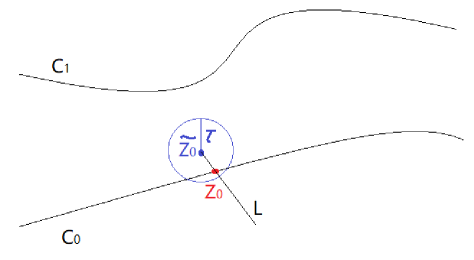
Figure 1: The associated exact point of an approximate point of the curve.

Next, we recall a result proved in [21] (Theorem 3.9).

Lemma 2.2.

Let $\sigma_{0}$ be the smallest singular value of $\mathcal{J}_{F}(z_{0})$. Let $\rho\geq 1$ and $\omega(\rho):=\sqrt{2\left(2\,\rho-1\right)\left(2\,\rho-2\,\sqrt{\rho\,\left(\rho-1\right)}-1\right)}$. Note that $\omega(\rho)$ is a monotone decreasing function with limit $1$ as $\rho\rightarrow+\infty$. Assume that $2\rho>3\omega$ holds (which is true for any $\rho\geq 1.6$). Let $\mu=\sqrt{n(n-1)}$ and $\displaystyle s_{0}=\frac{\sigma_{0}}{2\mu\rho_{0}}$, $\rho_{0}\geq 1.6$.

As illustrated in Fig. 2, let $L_{0}$ be a hyperplane which is perpendicular to the tangent line of $V_{\mathbb{R}}(F)$ at $z_{0}$ of distance $s_{0}$ to $z_{0}$. Let $z_{1}$ be a zero of $V_{\mathbb{R}}(F)\cap L_{0}$. Then $z_{1}$ is on the same component with $z_{0}$ if and only if

$$\|{z}_{1}-{z}_{0}\|_{2}<\omega(\rho_{0})\cdot s_{0}.$$ (1)

Now, let $L_{1}$ be a hyperplane which is perpendicular to the tangent line of $V_{\mathbb{R}}(F)$ at $z_{1}$ of distance $s_{1}$ to $z_{1}$ such that $z_{0}$ is a zero of $V_{\mathbb{R}}(F)\cap L_{1}$. Let $\sigma_{1}$ be the smallest singular value of $\mathcal{J}_{F}(z_{1})$. If there exists a $\rho_{1}\geq 1.6$ such that $\displaystyle s_{1}=\frac{\sigma_{1}}{2\mu\rho_{1}}$, by Lemma 2.2, $\|{z}_{1}-{z}_{0}\|_{2}<\omega(\rho_{1})\cdot s_{1}$ holds, as $z_{0}$ is on the same component with $z_{1}$. If such $\rho_{1}$ does not exist, we can always increase the value of $\rho_{0}$, thus reduce the step size $s_{0}$ such that the condition $\rho_{1}\geq 1.6$ is satisfied. Indeed, by Weyl’s theorem [37], $|\sigma_{1}-\sigma_{0}|\leq\|\mathcal{J}(z_{1})-\mathcal{J}(z_{0})\|_{2}$. By Lemma 1 of [30], $\|\mathcal{J}(z_{1})-\mathcal{J}(z_{0})\|_{2}\leq\mu\|{z}_{1}-{z}_{0}\|_{2}$. Thus $|\sigma_{1}-\sigma_{0}|\leq\mu\|{z}_{1}-{z}_{0}\|_{2}$. As $z_{1}$ approaches $z_{0}$, reducing $s_{1}$ implies increasing $\rho_{1}$.

To sum up, one can find $\rho_{i}\geq 1.6$ such that $\displaystyle s_{i}=\frac{\sigma_{i}}{2\mu\rho_{i}}$ and $\|{z}_{1}-{z}_{0}\|_{2}<\omega(\rho_{i})\cdot s_{i}$, for $i=0,1$. Let $\rho^{*}={\rm min}(\rho_{0},\rho_{1})\geq 1.6$. Let $h=\|{z}_{1}-{z}_{0}\|_{2}$. We define a cone with $z_{0}$ as the apex, the tangent line at $z_{0}$ as the axis, and the angle deviating from the axis being $\displaystyle\theta:=\arccos\bigg{(}\frac{1}{\omega(\rho^{*})}\bigg{)}$. By above analysis, the curve from $z_{0}$ to $z_{1}$ must be in this cone when the step size is small. Similarly, we can construct another cone with $z_{1}$ as the apex, the tangent line at $z_{1}$ as the axis, and the angle deviating from the axis being $\displaystyle\theta:=\arccos\bigg{(}\frac{1}{\omega(\rho^{*})}\bigg{)}$, such that it contains the curve from $z_{1}$ back to $z_{0}$. Figure 2 illustrates the two cones and the curve contained in them.

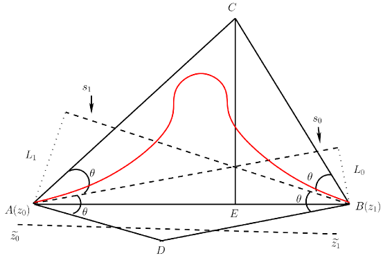
Figure 2: A 2D image illustrating the intersection of two cones.

From Figure 2, we know that $|CE|<|AE|\tan(2\theta)$ and $|CE|<|EB|\tan(2\theta)$ hold. Since $|AE|+|EB|=h$, we deduce that $\displaystyle|CE|<\frac{h}{2}\tan(2\theta)=\frac{h}{2}\tan\bigg{(}2\arccos\bigg{(}1/\omega(\rho_{*})\bigg{)}\bigg{)}$.

To summarize, we have the following lemma.

Lemma 2.3.

Use notations in the above analysis, let ${\cal C}_{z_{0}z_{1}}$ be the curve segment between $z_{0}$ and $z_{1}$ in $V_{\mathbb{R}}(F)$. Let $\sigma={\rm max}(\sigma_{0},\sigma_{1})$. The Hausdorff distance between $C_{z_{0}z_{1}}$ and the segment $\overline{{z}_{0}{z}_{1}}$ is at most $\displaystyle\frac{\omega(\rho_{*})\sigma}{4\mu\rho_{*}}\tan\bigg{(}2\arccos\bigg{(}\frac{1}{\omega(\rho_{*})}\bigg{)}\bigg{)}$.

In practice, $\rho_{1}$ and $z_{1}$ cannot be obtained exactly as before. But one can always apply interval arithmetic to obtain an approximation $\mathaccent 869{z_{1}}$ such that the associated exact point of $\mathaccent 869{z_{1}}$, called $z_{1}$ satisfies Lemma 2.3.

Assume that $\|z_{1}-\mathaccent 869{z_{1}}\|_{2}\leq\tau$. As before, by Weyl’s theorem [37] and Lemma 1 of [30], we have $\sigma_{i}\leq\mu\tau+\mathaccent 869{\sigma_{i}}$, $i=1,2$. Let $\mathaccent 869{\sigma}={\rm max}(\mathaccent 869{\sigma_{0}},\mathaccent 869{\sigma_{1}})$. Combining with Lemma 2.3, we have the following result.

Theorem 2.4.

The Hausdorff distance between $C_{z_{0}z_{1}}$ and the segment $\overline{\mathaccent 869{z}_{0}\mathaccent 869{z}_{1}}$ is at most

$$\tan\bigg{(}2\arccos\bigg{(}\frac{1}{\omega(\rho_{*})}\bigg{)}\bigg{)}\frac{\omega(\rho_{*})}{4\mu\rho_{*}}(\mu\tau+\mathaccent 869{\sigma})+\tau,$$

which is no greater than $\displaystyle 1.082\tau+0.082\frac{\mathaccent 869{\sigma}}{\mu}$ since $\rho_{*}\geq 1.6$.

2.3 Handling singularities

It is a well known fact that tracing a curve near singularities is difficult, as illustrated in Fig 3.

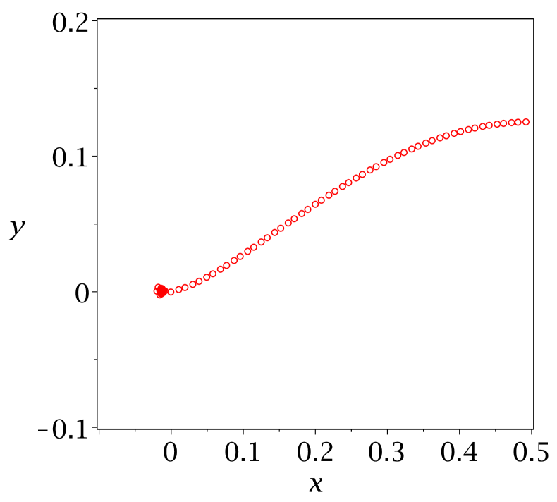
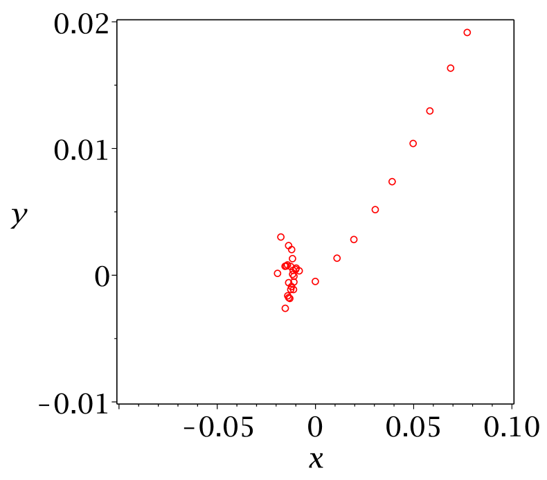
Figure 3: Tracing the curve near a singular point.

The left subfigure illustrates tracing the zero of $f={y}^{2}-\left(-{x}^{2}+x\right)^{3}$ starting with a regular point, where the right subfigure zooms in the part of the left subfigure near the origin, which is a singular point. We see that it may be difficult for curve tracing to escape out of the area near the origin, as near the origin, Newton’s method requires to solve a linear system $Az=b$ with a very large condition number. As a result, the errors are radically amplified.

Even worse, the topology of the curve near singularities is not numerically stable, as illustrated by Example 2.5.

Example 2.5.

Let $f:=x^{2}-y^{2}$. A slight perturbation of its coefficients changes completely the local topology near its singular point $(0,0)$, as depicted in Fig. 4.

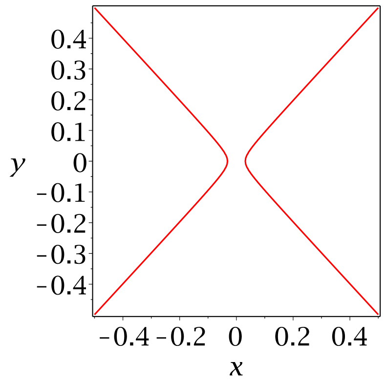
Plot of $f-0.001$.

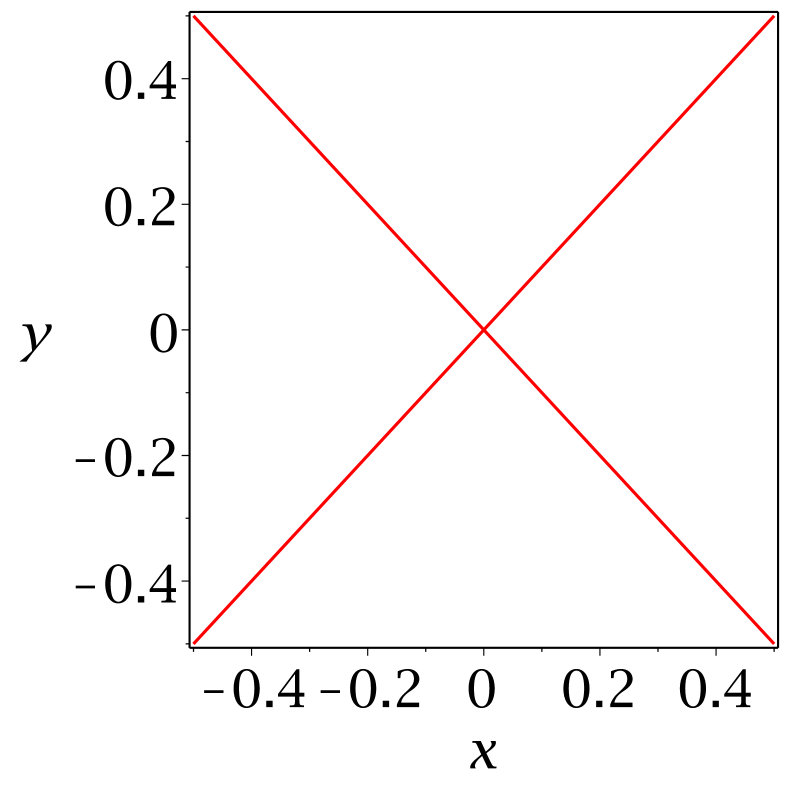
Plot of $f$.

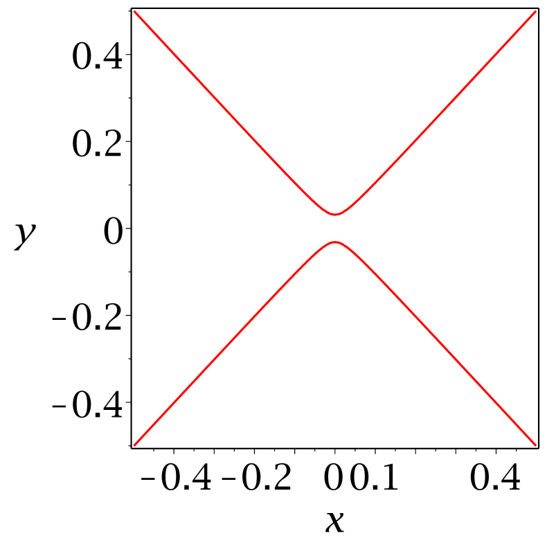
Plot of $f+0.001$.

Figure 4: Plot of $f$ and its perturbations.

So instead of tracing through a singular point, we bypass it. Before presenting an algorithm, we first use a simple example to illustrate the main idea.

Example 2.6.

Consider the polynomial $f:=6\,x{y}^{7}+85\,{x}^{4}{y}^{3}-60\,{x}^{2}{y}^{5}-32\,{x}^{2}{y}^{3}+14\,{x}^{4}-35\,{y}^{4}.$ Its real zero set is displayed in Fig. 5 as the red curve.

It has three connected components inside the box $-3\leq x\leq 3,-4\leq y\leq 2$. The component on the top has an isolated singular point $(0,0)$, colored in green. To plot this component, we first draw a circle centered at the origin, which has four intersection points with the curve, colored in black. Then we trace the four branches starting with the four black points until meeting the boundary. Next we plot the component at the left bottom corner. To do that, we start with a blue point, which is an intersection point of the curve with a boundary of the box, and trace the curve until meeting a boundary of the box. At last, we plot the closed component at the right bottom corner. To do that, we compute critical points of the curve in $x$-direction and get two yellow points. Starting with any point of them, trace the curve until meeting the point itself. Finally we plot the singular point. See the right subfigure of Fig. 5 for a visualization of the approximation.

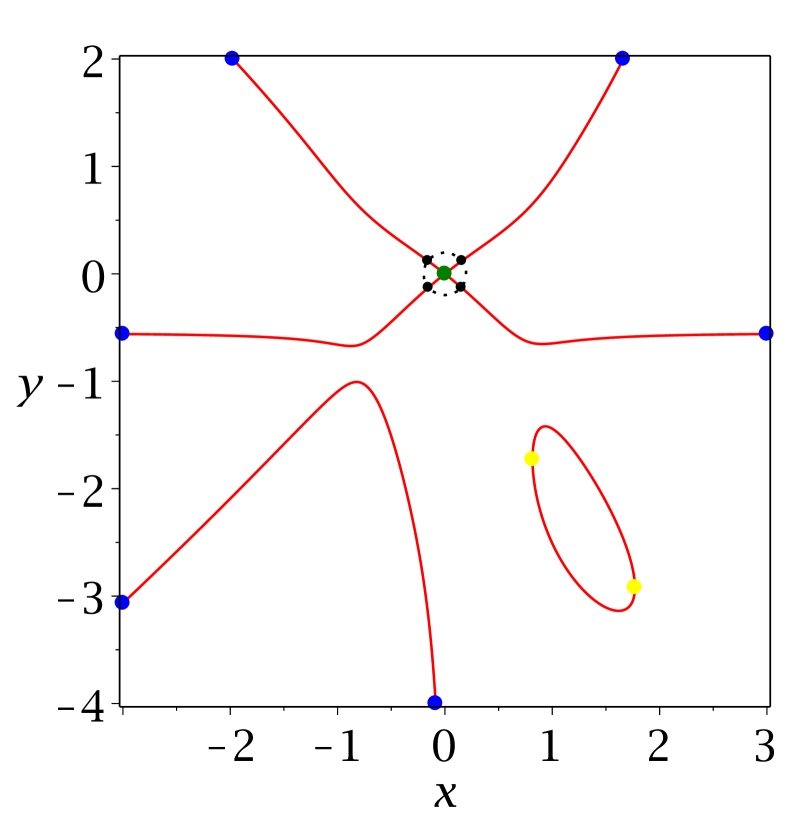
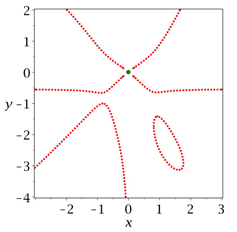
Figure 5: Left: the curve and key points. Right: an approximation of the curve ($\varepsilon=0.4$).

Note that the above procedure plots the whole curve inside the box except the part in a small neighborhood of the origin, which is simply replaced by a point. Such an approximation is numerically more stable than describing exactly the topology near the origin, as illustrated by Example 2.5. Moreover, in applications such as solving parametric polynomial systems, the curve is a border curve and such an approximation suffices to answer exactly the number of real solutions of the parametric system in an open cell of the complement of the curve.

Algorithm ApproxPlotBase

Input: a finite set of polynomials $F=\{f_{1},\ldots,f_{n-1}\}\in\mathbb{Q}[x_{1},\ldots,x_{n}]$; a bounding box $B\subset\mathbb{R}^{n}$, and a given precision $\varepsilon$.

Output: an $\varepsilon$-approximation of $V_{\mathbb{R}}(F)$.

Assumptions: $(i)$ the singular points are not on the boundary of the box $B$; $(ii)$ the distance between two singular points is at least $\varepsilon$;

Compute the singular points $S_{0}={\sf SingularPoints}(F,B)$.

Compute the intersection of the curve with spheres centered at the singular points with radius less than $\varepsilon/2$ . Set $S_{1}$ to be the set of these points, called fencing points (around singular points). We denote by ${\sf FencingPoints}$ an operation to compute such points. Let $\Delta$ be the set of balls associated with these spheres.

Compute the intersection of the curve with the boundaries. Set $S_{2}$ to be the set of these points.

Compute the witness points of $V_{R}(F)$ (inside $B$) $S_{3}:={\sf WitnessPoints}(F,B)$. Remove from $S_{3}$ points that are already inside any balls in $\Delta$.

Starting with a point in $S_{1}$, trace the curve robustly based on Theorem 2.4 until meeting ($\varepsilon$-close to) a point in $S_{1}$ or $S_{2}$. Remove the starting point and the corresponding points met in $S_{1}$ or $S_{2}$. Repeat Step $(5)$ until $S_{1}=\emptyset$. Let the resulting set of polygonal chains be $P_{1}$.

If $S_{2}\neq\emptyset$, starting with a point in $S_{2}$, trace the curve robustly until meeting a point in $S_{2}$. Remove the point met in $S_{2}$. Repeat Step $(6)$ until $S_{2}=\emptyset$. Let the resulting set of polygonal chains be $P_{2}$.

Remove points of $S_{3}$ which are already on the computed curve.

If $S_{3}\neq\emptyset$, starting with a point in $S_{3}$, trace the curve robustly until closed curves are found. Remove point met during the tracing from $S_{3}$. Repeat Step $(8)$ until $S_{3}=\emptyset$. Let the resulting set of polygonal chains be $P_{3}$.

Return $S_{0}\cup P_{1}\cup P_{2}\cup P_{3}$.

Remark 2.7.

Assumption $(i)$ can relaxed by slightly shrinking or expanding the box. Assumption $(ii)$ can be relaxed by grouping the singular points into clusters. See Section 3 for details.

Theorem 2.8.

One can control errors of staring points and prediction-correction in the above tracing algorithm, such that Algorithm ApproxPlotBase computes an $\varepsilon$-approximation of $V_{\mathbb{R}}(F)$.

Proof 2.9.

We remark that to obtain an $\varepsilon$-approximation of the curve, one must have one witness point from each connected component of the curve. If a component is a solitary point, it must be in $S_{0}$. For the other components which intersect with the boundary or have singular points, the starting points are in $S_{2}$ and $S_{1}$ respectively. Note that although $S_{3}$ may not contain witness points for every connected component of $V_{\mathbb{R}}(F)$, it must contain at least one witness points for each smooth closed component of $V_{\mathbb{R}}(F)$. By the assumptions, the polynomial systems with zero sets $S_{i}$, $i=0,\ldots,3$ are all zero-dimensional. If the interval Newton method [38] converges, the error of solving these zero-dimensional systems and the error of Newton iterations (in the corrector step), as well as the distance between the curve and the polygonal chains can be controlled to be much less than $\varepsilon$ by Theorem 2.4. Otherwise, one can reduce the step size until the $\alpha$-theory [23, 24] guarantees the convergence of Newton iterations. Moreover, by Theorem 2.4, curve jumping can be avoided. Finally note that in the $\varepsilon/2$-neighborhood of the singular points, the distance between the curve and the polygonal chains are less than $\varepsilon$. Thus, an $\varepsilon$-approximation of $V_{\mathbb{R}}(f)$ can be computed.

3 Improvements

In this section, we propose several strategies for improving the numerical stability of the tracing algorithm in last section. These improvements lead to a practical algorithm presented in next section.

3.1 Choice of tracing direction

This first strategy is plotting the curve in the direction away from the singular points rather than towards the singular point. In practice, the former can better avoid curve jumping, as illustrated by Fig. 6.

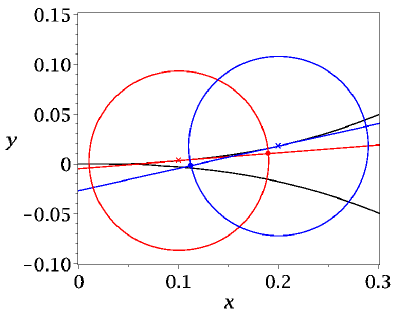
Figure 6: Jump is more likely to happen when tracing towards singular points.

In this figure, the black curve is the locus of $f:=x^{5}-y^{2}.$ To trace the upper branch, we have two possible starting points, namely the red $\times$ point, say $z_{0}$, and the blue $\times$ point, say $z_{1}$. If we start from $z_{0}$ and move in the tangent direction towards $z_{1}$ in step size $0.09$, we get a red $\bullet$ point close to the upper branch, with which as an initial point, Newton iteration converges to a point still in the upper branch. However, if we start from $z_{1}$ and move in the tangent direction towards $z_{0}$ in step size $0.09$, we get a blue $\bullet$ point close to the lower branch. As a result, Newton iteration converges to a point in the lower branch.

This justifies why we first start with fencing points around singular points instead of the boundary points to trace the curve, as shown by Line $20$ of Algorithm 1. However, this first strategy does not consider the situation that there are two singular points in the same component, for which a try-stop-resume strategy is needed, as illustrated by examples in next subsection.

3.2 A try-stop-resume tracing strategy

Example 3.1.

Consider again the polynomial $f:={y}^{2}-\left(-{x}^{2}+x\right)^{3}.$ It is a closed curve with two singular points $(0,0)$ and $(1,0)$.

In Fig. 7, the algorithm first plots the red points starting from two fencing points near $(0,0)$ and stops when the singular values drop (at the two $\times$ points, which are called front points). See also line $37$ of Algorithm 2 for an implementation. It then starts from the two fencing points near $(1,0)$ and plots the blue points, which happen to meet the front points before singular values drop. Checking if front points are met is implemented in Algorithm 2 from line $32$ to $35$.

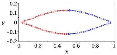
Figure 7: Try to plot the curve away from the singular points and stop when singular values drop.

The above example does not need the resuming step. Consider another one.

Example 3.2.

Consider

$$\begin{array}[]{rl}f:=&-3375\,{y}^{14}-4050\,{x}^{4}{y}^{9}+108\,{y}^{13}-1215\,{x}^{8}{y}^{4}-648\,{x}^{2}{y}^{9}\\ &+2700\,{y}^{11}+1620\,{x}^{4}{y}^{6}+1296\,{x}^{4}{y}^{5}-5400\,{x}^{2}{y}^{7}-3240\,{x}^{6}{y}^{2}\\ &-1170\,{y}^{8}-864\,{x}^{6}y-810\,{x}^{4}{y}^{3}-720\,{x}^{2}{y}^{4}+4000\,{y}^{6}\\ &+2400\,{x}^{4}y+540\,{y}^{5}+720\,{x}^{4}-1080\,{x}^{2}y-135\,{y}^{2}+800.\end{array}$$

The locus of $f$ is visualized in Fig. 8. During the try phase, the algorithm starts with the fencing points at the bottom and plots the red point. After all red parts have been plotted, it resumes and plots the blue parts and finally the green parts. In this way, it avoids directly tracing from the left singular point to the right one. The resuming step is implemented at line $21$ in Algorithm 1, which calls Algorithm 2 with the value of first argument $cwp$ replaced by front points ($front$).

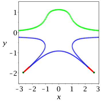
Figure 8: Try to plot the curve away from the singular points and stop when singular values drop and resume.

3.3 Handling clustered singular points

The third improvement is to take clustered singular points into consideration. We borrow the notion of natural cluster from [34] on Voronoi vertices. Given a set $S$ of singular points of $Z_{\mathbb{R}}(f)$ in a bounding box $B$. For any disk $D(z,r)$ centered at $z$ of radius $r$, let $\Delta_{S}(z,r)$ be the set of points in $S$ contained in $D(z,r)$. If it is not empty, we call it a cluster of $S$. It is called a natural cluster if $D(z,r)$ and $D(z,3r)$ contains exactly the same set of points of $S$. We call $D(z,r)$ an associated disk of $\Delta_{S}(z,r)$. Note that the associated disks of two different natural clusters are disjoint and the distance between their centers are at least $3r$. For a given $S$, it is easy to generate a set of disjoint natural clusters and their associated disks. For instance, one can first sort the singular points in an ascending order by the minimal distances from the point to the other points. One can then check if the points form natural clusters of radius $r$ incrementally. If not, we reduce the radius $r$ by half and repeat the above procedure. Let $d$ be the minimal distances among points in $S$. One can always obtain natural clusters of radius less than $d/3$. Let ${\sf NatualClusters}$ be such an operation, which takes $S$ and $\varepsilon/2$ as input and return a set ${\cal C}$ of natural clusters of radius $\delta$. It is called at line $6$ of Algorithm 1. Let’s consider an example.

Example 3.3.

Let $g:=-28\,{x}^{4}yz+58\,x{y}^{5}-65\,x{y}^{2}{z}^{3}+23\,{x}^{4}y+24\,{x}^{3}yz-64\,{x}^{2}{z}^{3}-32\,xy{z}^{3}-72\,x{y}^{2}z+6\,{z}^{4}+56\,xyz+1$ and $f$ be the discriminant of $g$ w.r.t. $z$, which is an irreducible polynomial in $\mathbb{Q}[x,y]$. A visualization of it in the box $-1\leq x\leq 1,-1\leq y\leq 1$ is depicted in Fig. 9. The two points $(-0.9257645305e-1,0.7100519895)$ and $(-0.6009009066e-1,0.7790657631)$ on the top of Fig. 9 form a natural cluster of radius $0.1$. Note that near the left bottom corner of the box, the curve is plotted with a larger step size than the other parts.

A second example for natural clusters is illustrated by Fig. 12 in Section 5.

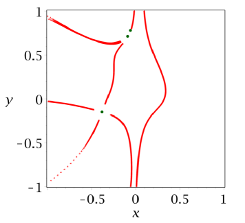
Figure 9: Plotting the curve with the help of natural clusters.

3.4 Computing singular points under perturbation

The fourth improvement is to take into account the fact that sometimes the coefficients of input polynomials may be given approximately. As a result, as illustrated by an example earlier, an exact computation of singular points may be impossible. Consequently, we may fail to find Jacobian numerically singular parts of the curve if we directly compute the singular points. Thus, in the following, we propose a method to numerically computing singular points.

We start by considering the case of plane curve defined by a polynomial $f\in\mathbb{R}[x_{1},x_{2}]$. We are interested in computing an $\varepsilon$-approximation of $V_{\mathbb{R}}(f)$. Suppose that we are given a $\tau\leq\varepsilon$ perturbation to $f$ and let $g=f-\tau$ be the perturbed polynomial. Assume that $V_{\mathbb{R}}(g)$ is nonempty and the Hausdorff distance between $V_{\mathbb{R}}(g)$ and $V_{\mathbb{R}}(f)$ is $\ll\varepsilon$.

According to Sard’s theorem, for almost all such $\tau$, any point of $V_{\mathbb{R}}(g)$ is a regular point of the map $f$, which implies that $V_{\mathbb{R}}(g)$ is a smooth manifold of dimension one (we assumed that $V_{\mathbb{R}}(g)$ is nonempty).

Let $S:=\{q\mid q\mbox{~{}is a critical point of~{}}g\mbox{~{}and~{}}|g(q)|\leq\varepsilon\}$. Let $p$ be a singular point of $f$. We have $|g(p)|=|f(p)-\tau|=|\tau|\leq\varepsilon$, which implies that $p\in S$. On the other hand, since $d_{H}(V_{R}(f),V_{\mathbb{R}}(g))\ll\varepsilon$, we have $d_{H}(p,V_{\mathbb{R}}(g))\ll\varepsilon$. Thus from a given polynomial $g$, we get an approximation point $p$ of $g=0$ ($d_{H}(p,V_{\mathbb{R}}(g))\ll\varepsilon$), which turns to be a true singular point of its nearby polynomial $f=g+\tau$. We call such point a “pseudo singular point” of $V_{\mathbb{R}}(g)$. Note that the set $S$ contains all such points (and possibly others).

To summarize, if the constant coefficient of $f$ is slightly perturbed, in practice we can compute $S$ and use the point of $S$ to compute fencing points.

In general, let $F=\{f_{1},\ldots,f_{n-1}\}$ be the set of polynomials defining the curve. Let $G=\{g_{1},\ldots,g_{n-1}\}$ be a small perturbation of $F$. Finding “pseudo singular points” of $V_{\mathbb{R}}(G)$ is a difficult problem. Instead, we propose the following heuristic strategy to compute $S$, which works well in practice.

Let $J$ be the Jacobian matrix of $G$. Let $J_{i}$, $i=1,\ldots,n$ be the submatrix of $J$ by deleting $i$-th column. Let $\Delta_{i}$ be the determinant of $J_{i}$. Then the critical points of $G:\mathbb{R}^{n}\rightarrow\mathbb{R}^{n-1}$ are the zeros of the system $\Delta:=\{\Delta_{1},\ldots,\Delta_{n}\}$, whose dimension in general is expected to be $n-2$. Let $E_{i}:=\{g_{1},\ldots,g_{i-1},g_{i+1},g_{n-1}\}\cup\Delta$. Let $S:=\cup_{i=1}^{n-1}\{q\mid q\in V_{\mathbb{R}}(E_{i})\mbox{~{}and~{}}|g_{i}(q)|\leq\varepsilon\}$. We denote by ${\sf PseudoSingularPoints}$ an operation to compute such $S$, which is called by Algorithm 1 at line $5$. It is possible that $S$ has identical points or points very close, which can be resolved by the natural cluster technique presented in last subsection.

4 A practical algorithm

In Section 2, we presented a theoretical algorithm to compute an $\varepsilon$-approximation of a curve, which may not be practical due to the small step size chosen. In practice, one has to make a compromise between efficiency and accuracy. Based on the improvement strategies in last section, next we develop a more practical algorithm. Instead of preventing curve jumping, in the algorithms below, we maintain a simple data structure to record if a start point has been visited. If a point is visited more than once, then there is a possible curve jumping.

Remark 4.1.

The main features of Algorithm ApproxPlot, such as tracing the curve away from the singular points, and grouping the singular points into natural clusters and the try-and-resume strategy has been explained in last section. Another feature of the algorithm is to detect curve jumping by counting the number of times that a fencing point or boundary point is visited.

To achieve this, each fencing point, boundary point, or new front point generated due to the drop of singular value, is treated as an object with four attributes $(q,v,s,c)$, where $q$ is the point itself, $v$ is the tracing direction, $s$ is the singular value of $J_{F}(q)$ and $c$ counts the times that $q$ is visited. For an object $ob$, the notation $ob.q$ means taking the value of the attribute $q$. Each $q$ should be visited one and only one time. If its visiting time $c>1$, there is a possible curve jumping at $q$. It is easy to check that if there is no curve jumping, after executing Algorithm PlotMain, the value of any $c$ (counting visiting times of a fencing point or boundary point) can not be greater than $1$. Moreover, if the numerical errors are well controlled, after executing line $22$ of Algorithm ApproxPlot, all the points in $rwp$ will only be on the closed components of the curve. Thus the value of any $c$ can not increase after executing Algorithm PlotOval. Finally we remark that the algorithm may not detect curve jumping errors caused by exchanging branches during tracing.

Input: A finite set of polynomials $F=\{f_{1},\ldots,f_{n-1}\}\in\mathbb{R}[x_{1},\ldots,x_{n}]$. A bounding box $B\subset\mathbb{R}^{n}$. A precision $\varepsilon>0$.

Output: An $\varepsilon$-approximation of $F^{-1}(0)$ in $B$.

1 begin

2       if $F$’s coefficients are known exactly then

3             let $S_{0}={\sf SingularPoints}(F,B)$;

4            

5       else

6             let $S_{0}={\sf PseudoSingularPoints}(F,B,\varepsilon)$;

7            

8      let ${\cal C},\delta:={\sf NatualClusters}(S_{0},\varepsilon/2)$;

9       $cwp:=\emptyset$; $bwp:=\emptyset$;

10       for each natural cluster $C\in{\cal C}$ do

11             let $p$ be the center point of $C$;

12             for each $q\in{\sf FencingPoints}(p,\delta)$ do

13                   let $s$ be the smallest singular value of ${\mathcal{J}}_{F}(q)$;

14                   let $v:=q-p$; let $c:=0$; add $(q,v,s,c)$ to $cwp$;

15                  

16            

17      for each point $q$ of $F^{-1}(0)\cap\partial B$ do

18             let $s$ be the smallest singular value of ${\mathcal{J}}_{F}(q)$;

19             let $v$ be the tangent vector of $F^{-1}(0)$ towards the interior of $B$;

20             let $c:=0$; add $(q,v,s,c)$ to $bwp$;

21            

22      let $\Delta$ be the union of balls associated with the natural clusters;

23       rescale the coefficients of $F$ if necessary;

24       set $rwp:={\sf WitnessPoints}(F,B)\setminus\Delta$;

       /* Note that below the function PlotMain is called multiple times with different arguments and flags. */

25       $S_{1},front:={\sf PlotMain}(F,B,cwp,bwp,rwp,\delta,try)$;

26       $S_{2}:={\sf PlotMain}(F,B,front,bwp,rwp,\delta,resume)$;

27       $S_{3}:={\sf PlotMain}(F,B,bwp,cwp,rwp,\delta,boundary)$;

28       $S_{4}:={\sf PlotOval}(F,B,rwp,cwp\cup bwp,\delta)$;

29       if $F$’s coefficients are known exactly then

30             return $\{\cup_{i=0}^{4}S_{i}\}$;

31            

32       else

33             return $\{\cup_{i=1}^{4}S_{i}\}$;

34            

35      

36

Algorithm 1 ${\sf ApproxPlot}$

1 begin

2       $S:=\emptyset$; $front:=\emptyset$;

3       for $j$ to $|cwp|$ do

4             $P:=\emptyset$; $(q,v,s,c):=cwp[j]$;

5             if $cwp[j].c>0$ then next; else $cwp[i].c:=1$;

6             $mb:=false$; $mc:=false$; $mf:=false$;

7            

8            while $q\in B$ do

9                  

10                  $s^{\prime}:=s$; $q^{\prime}:=q$; $v^{\prime}:=v$; $P:=P\cup\{q\}$;

11                   choose step size $h\leq\delta/2$ according to $\delta$ and $s$;

                   $q:=q+hv$;// Predictor step

12                  

13                  with $q$ as initial point, apply Newton iterations to update $q$;

14                   let $s$ be the smallest singular value of $J_{F}(q)$; let $v:={{t}}(J_{F}(q))$;

15                   if $v\bullet v^{\prime}<0$ then  $v:=-v$ ;

16                   remove any element of $rwp$ on $\overline{q^{\prime}q}$;

17                   for $i$ to $|bwp|$ do

18                         if $(bwp[i].v)\bullet v<0\wedge bwp[i].q\in\overline{q^{\prime}q}$ then

19                               if $bwp[i].c>0$ then

20                                     report curve jump error;

21                                    

22                               else

23                                     $P:=P\cup\{bwp[i].q\}$;

24                                    

25                              $mb:=true$; $bwp[i].c:=bwp[i].c+1$; break;

26                              

27                        

28                  if $mb$ then break;

29                  

30                  for $i$ to $|cwp|$ do

31                         if $i\neq j$ and $(cwp[i].v)\bullet v<0$ and $cwp[i].q\in\overline{q^{\prime}q}$ then

32                               if $cwp[i].c>0$ then

33                                     report curve jump error;

34                                    

35                               else if tag is ’resume’ or ’try’ then

36                                     $P:=P\cup\{cwp[i].q\}$;

37                                    

38                              $mc:=true$; $cwp[i].c:=cwp[i].c+1$; break;

39                              

40                        

41                  if $mc$ then break;

42                  

43                  if tag=’try’ then

44                         for $i$ to $|front|$ do

45                               if $front[i].v\bullet v<0$ and $front[i].q\in\overline{q^{\prime}q}$ then

46                                     $P:=P\cup\{front[i].q\}$; $mf:=true$; remove $front[i]$ from $front$;

47                                     break;

48                                    

49                              

50                        if $mf$ then break;

51                        

52                        if $s<s^{\prime}$ then

53                               add $(q,v,s,0)$ to $front$;break;

54                              

55                        

56                  

57            $S:=S\cup\{P\}$;

58            

59      if tag=’try’ then return $S$, $front$ else return $S$;

60

Algorithm 2 ${\sf PlotMain}(F,B,cwp,bwp,rwp,\delta,tag)$

1 begin

2       $S:=\emptyset$;

3      

4      while $rwp\neq\emptyset$ do

5             $P:=\emptyset$;

6             choose $p\in rwp$ and set $rwp:=rwp\setminus\{p\}$; $k:=0$; $q:=p$;

7             let $s$ be the smallest singular value of $J_{F}(q)$;

8             let $v:={{t}}(J_{F}(q))$;

9            

10            $mt:=false$;

11            

12            while $q\in B$ do

13                  

14                  $k:=k+1$; $q^{\prime}:=q$; $v^{\prime}:=v$; $P:=P\cup\{q\}$;

15                  

16                  choose step size $h\leq\delta/2$ according to $\delta$ and $s$;

17                  

18                  $q:=q+hv$;

19                  

20                  with $q$ as initial point, apply Newton iterations to update $q$;

21                  

22                  let $s$ be the smallest singular value of $J_{F}(q)$;

23                   let $v:={{t}}(J_{F}(q))$;

24                  

25                  if $v\bullet v^{\prime}<0$ then  $v:=-v$ ;

26                   if $k>2$ and $p\in\overline{q^{\prime}q}$ then

27                         break;

28                        

29                  remove any element of $rwp$ other than $p$ on $\overline{q^{\prime}q}$;

30                   for $i$ to $|wp|$ do

31                         if $(wp[i].v)\bullet v<0\wedge wp[i].q\in\overline{q^{\prime}q}$ then

32                               if $wp[i].c>0$ then

33                                     report curve jump error;

34                                    

35                              $mt:=true$; $wp[i].c:=wp[i].c+1$; break;

36                              

37                        

38                  if $mt$ then break;

39                  

40            $S:=S\cup\{P\}$;

41            

42      return $S$;

43      

44

Algorithm 3 ${\sf PlotOval}(F,B,rwp,wp,\delta)$

5 Experimentation

In this section, we provide some nontrivial examples to illustrate the effectiveness of our method. Example 5.1 is the discriminant of a random trivariate polynomial. Example 5.2 is the resultant of two random trivariate polynomials. To make a fair comparison with the Plots:-implicitplot command of Maple $18$, all polynomials are plotted using their irreducible factors.

We have implemented our algorithm in Maple. In the algorithms of last section, there are several places where ones needs to solve zero-dimensional polynomial systems, namely computing singular points, computing fencing points around singular points, computing boundary points and computing witness points. For the first three, we find that it is more robust to call a symbolic solver and use RootFinding:-Isolate of Maple. For the last one, we find it is more efficient to use homotopy based methods and we implemented a Maple interface to hom4ps2 [39]. The experimental results in this section were obtained on an Fedora laptop (Intel i7-7500U CPU @ 2.70GHz, 16.0 GB total memory). A preliminary implementation of ApproxPlot is available at http://www.arcnl.org/cchen/software.

5.1 Visualizing planar curve

Example 5.1.

Let $f$ be the same polynomial as in Example 3.3. Visualizations of $it$ by Plot:-implicitplot in Maple and ApproxPlot is depicted in Fig. 10. The option for Plot:-implicitplot is grid=[300,300], gridrefine=6, crossingrefine=4 and the time spent is $34.3$ seconds. The option for ApproxPlot is $\varepsilon=0.5$ and the time spent is $42.7$ seconds. For this example, the initial radius $\varepsilon/2$ suffices to dividing the $4$ singular points into $3$ natural clusters. The polynomial $f$ has branches very close to each other and the algorithm detects curve jumping.

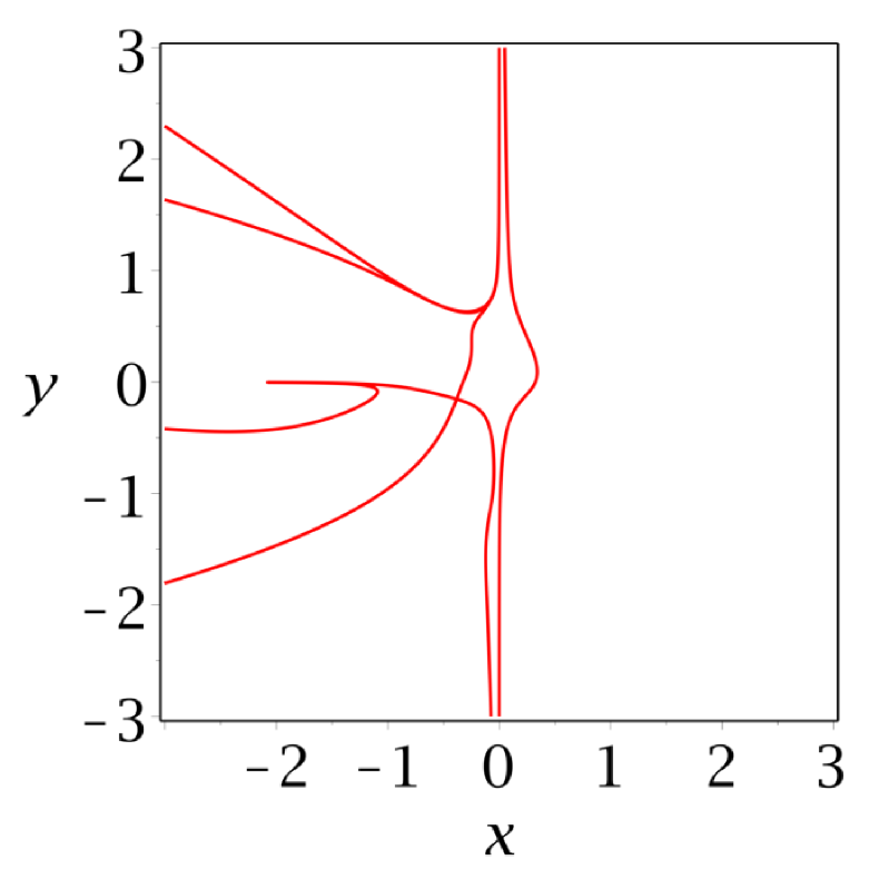
By Maple Plot:-implicitplot.

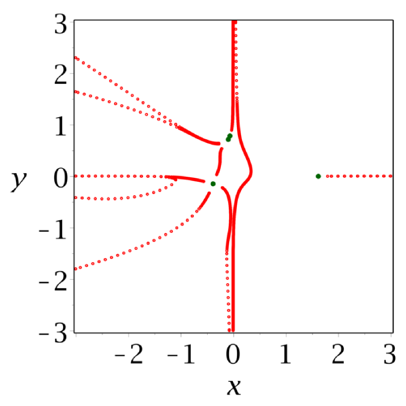
By ApproxPlot.

Figure 10: Visualization of Example 5.1.

Example 5.2.

Let $f_{1}:=72\,{y}^{2}{z}^{5}+26\,{x}^{2}y{z}^{3}-84\,{x}^{2}{y}^{2}-73\,x{z}^{2}+6,f_{2}:=-24\,{x}^{4}{z}^{2}-35\,y{z}^{3}+43\,y{z}^{2}-66\,{z}^{3}+3$. Let $f$ be the resultant of $f_{1}$ and $f_{2}$ w.r.t. $z$. A visualization of it is depicted in Fig. 11. The polynomial $f$ has branches very close to each other and the algorithm detects curve jumping. The option for Plot:-implicitplot is grid=[300,300],gridrefine=6,crossingrefine=6 and the time spent is $36.4$ seconds. The option for ApproxPlot is $\varepsilon=0.5$ and the time spent is $32.5$ seconds. For this example, the initial radius for finding clusters is $0.25$, which finally gets updated to $0.0625$ to find $7$ natural clusters for $10$ singular points, see Fig. 12.

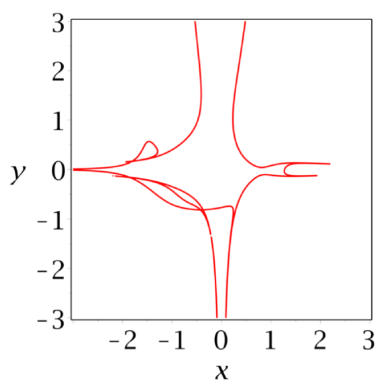
By Maple.

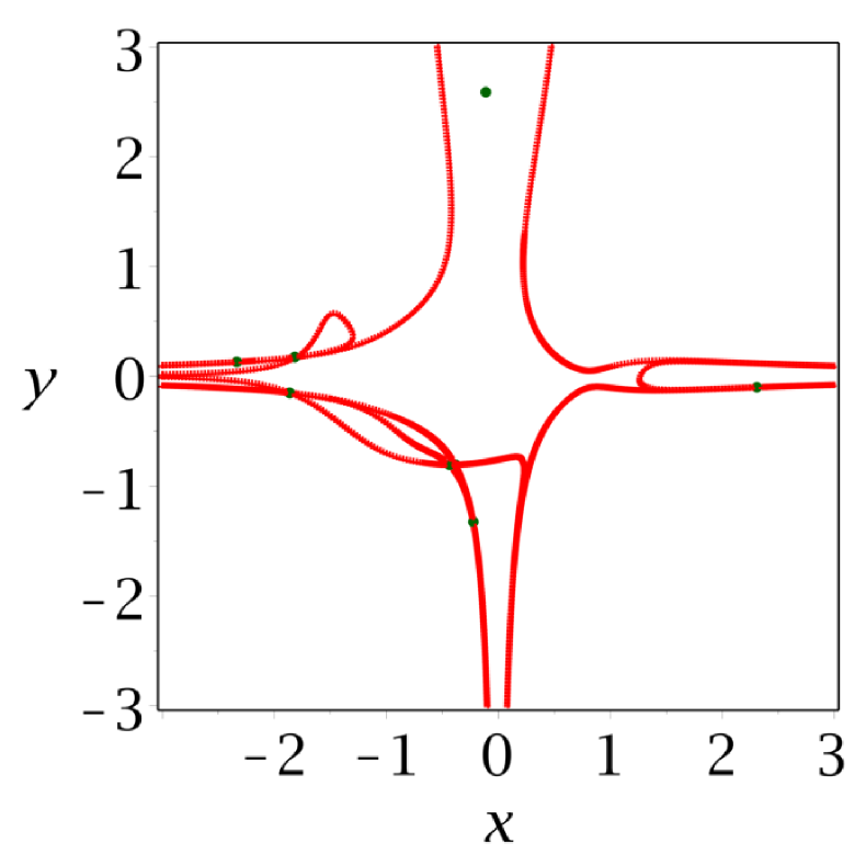
By ApproxPlot.

Figure 11: Visualization of Example 5.2.

The seven natural clusters.

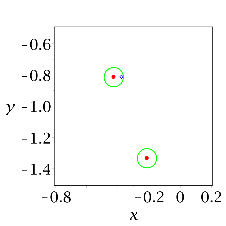
A close-up view of two natural clusters.

Figure 12: Natural clusters for Example 5.2.

5.2 Visualizing space curve

Example 5.3.

Let $f:=\{3\,{x}^{7}{y}^{4}z+{y}^{12}+{z}^{12}-{y}^{5}{z}^{6}-5\,{x}^{7}{y}^{2}z+5\,x{y}^{3}{z}^{6}-8\,{x}^{3}yz-8\,{y}^{3}-y{z}^{2}+10\}$ be a randomly generated trivariate polynomial. Let $\displaystyle F:=\bigg{\{}\frac{\partial f}{\partial z},\frac{\partial f}{\partial y}\bigg{\}}$. A visualization of it is depicted in Fig. 13. The option for plots:-intersectplot is $grid=[60,60,60]$ and the time spent is $33.5$ seconds. The option for ApproxPlot is $\varepsilon=0.2$ and the time spent is $22.2$ seconds. No curve jumping is reported by ApproxPlot. As we can see, Maple has issues when visualizing the parts on the plane $y=-3$ and $y=3$.

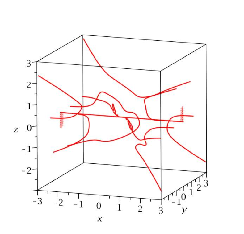
By Maple plots:-intersectplot.

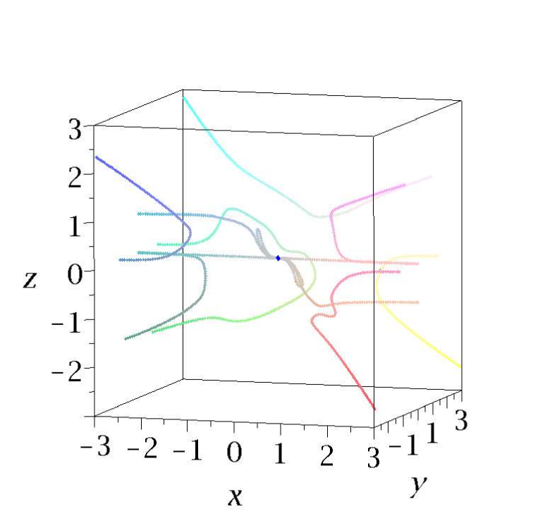
By ApproxPlot.

Figure 13: Visualization of Example 5.3.

Example 5.4.

Let $f:=-51\,{x}^{12}yz+31\,{x}^{4}y{z}^{8}+68\,{x}^{11}z-10\,{x}^{5}{y}^{4}{z}^{3}+{z}^{12}+91\,{x}^{5}{y}^{2}{z}^{3}-81\,{y}^{5}+10$ and $\displaystyle F:=\bigg{\{}f,\frac{\partial f}{\partial z}\bigg{\}}$. A visualization of it is depicted in Fig. 14. The option for plots:-intersectplot is $grid=[60,60,60]$ and the time spent is $40.5$ seconds. The option for ApproxPlot is $\varepsilon=0.2$ and the time spent is $27.3$ seconds. No curve jumping is reported by ApproxPlot. As we can see, Maple clearly has visualization issues.

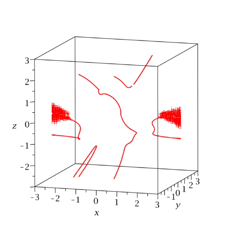
By Maple plots:-intersectplot.

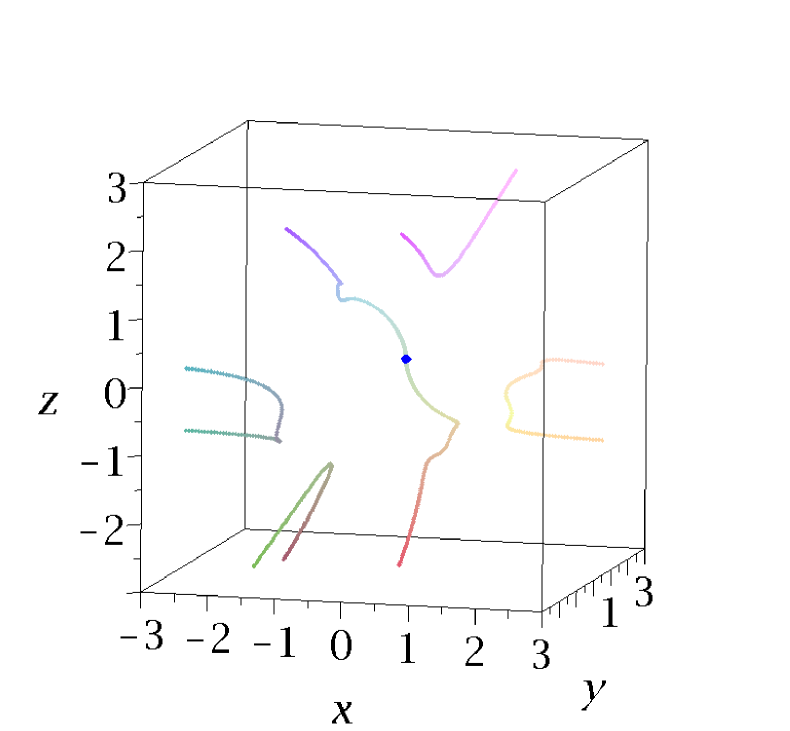
By ApproxPlot.

Figure 14: Visualization of Example 5.4.

Example 5.5.

We consider a famous surface called Barth Decic [40] defined by

$$\begin{array}[]{rl}f:=&8\,\left(-{r}^{4}{y}^{2}+{x}^{2}\right)\left(-{r}^{4}{z}^{2}+{y}^{2}\right)\left(-{r}^{4}{x}^{2}+{z}^{2}\right)\left({x}^{4}-2\,{x}^{2}{y}^{2}-2\,{x}^{2}{z}^{2}+{y}^{4}-2\,{y}^{2}{z}^{2}+{z}^{4}\right)\\ &+\left(3+5\,r\right)\left(-{w}^{2}+{x}^{2}+{y}^{2}+{z}^{2}\right)^{2}\left({x}^{2}+{y}^{2}+{z}^{2}-\left(2-r\right){w}^{2}\right)^{2}{w}^{2}\end{array}$$

and $\displaystyle F:=\bigg{\{}f,\frac{\partial f}{\partial z}\bigg{\}}$.

We consider the case that $w=1$ and $r=2$. The polynomial $\displaystyle\frac{\partial f}{\partial z}$ has two irreducible factors, one of them is $z$. Let $F_{1}=[f,z]$ and $\displaystyle F_{2}=\bigg{[}f,1/z\cdot\frac{\partial f}{\partial z}\bigg{]}$. We plot $F_{1}$ and $F_{2}$ separately and display them together. The option for plots:-intersectplot is $grid=[80,80,80]$ and the total time spent is $108.7+154.8=263.5$ seconds.

The option for ApproxPlot is $\varepsilon=0.1$ and the time spent is $1704.3$ seconds. No curve jumping is reported by ApproxPlot. A visualization of it is depicted in Fig. 15. As we can see, Maple clearly has visualization issues.

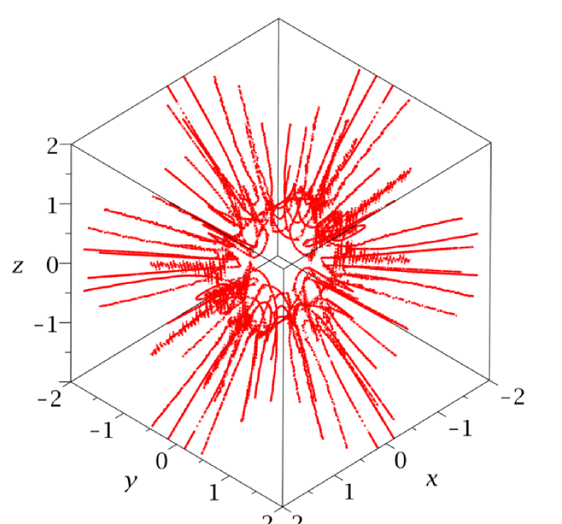
By Maple plots:-intersectplot.

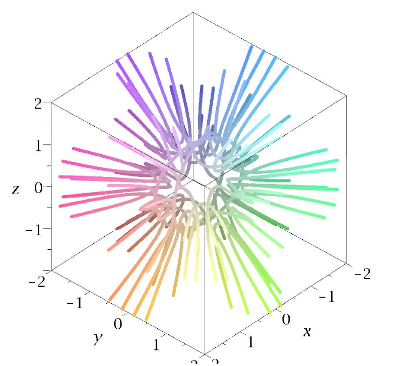
By ApproxPlot.

Figure 15: Visualization of Example 5.5.

Example 5.6.

We consider a famous surface called Barth Sextic [40] defined by $f:=4\,\left({r}^{2}{x}^{2}-{y}^{2}\right)\left({r}^{2}{y}^{2}-{z}^{2}\right)\left({r}^{2}{z}^{2}-{x}^{2}\right)-\left(1+2\,r\right)\left(-{w}^{2}+{x}^{2}+{y}^{2}+{z}^{2}\right)^{2}{w}^{2}$ and $\displaystyle F:=\bigg{\{}f,\frac{\partial f}{\partial z}\bigg{\}}$. Consider the case that $w=1$ and $\displaystyle r=\frac{\sqrt{5}+1}{2}$. The option for plots:-intersectplot is $grid=[100,100,100]$, $maxlev=8$ and the time spent is $107.7$ seconds. The option for ApproxPlot is $\varepsilon=0.1$. There are two ways to plot the curve by ApproxPlot. One is to use an approximate value of $r$ and plot the curve in $\mathbb{R}^{3}$. In such case, an exact computation shows that there are no singular points. As a result, there is curve jumping and some part of the curve is missing after tracing. Instead, we use the technique of pseudo singular points, and no curve jumping is reported. The time spent is $76.7$ seconds. Another method is to encode the algebraic number $r$ by its defining polynomial $r^{2}-r-1$. We then trace the curve defined by $\displaystyle\bigg{\{}f,\frac{\partial f}{\partial z}\bigg{\}},r^{2}-r-1$ in $\mathbb{R}^{4}$ and take its projection in $\mathbb{R}^{3}$. The time spent in this way is $118.3$ seconds. No curve jumping is reported by ApproxPlot. A visualization of the space curve is depicted in Fig. 16.

Example 5.7.

Consider $Endra\ss$ Octic surface [40] defined by

$$\begin{array}[]{rl}f:=&64\,\left(-{w}^{2}+{x}^{2}\right)\left(-{w}^{2}+{y}^{2}\right)\left(\left(x+y\right)^{2}-2\,{w}^{2}\right)\left(\left(x-y\right)^{2}-2\,{w}^{2}\right)\\ &-\bigg{(}-4\,\left(1+\sqrt{2}\right)\left({x}^{2}+{y}^{2}\right)^{2}+\left(8\,\left(2+\sqrt{2}\right){z}^{2}+2\,\left(2+7\,\sqrt{2}\right){w}^{2}\right)\left({x}^{2}+{y}^{2}\right)\\ &-16\,{z}^{4}+8\,\left(1-2\,\sqrt{2}\right){z}^{2}{w}^{2}-\left(1+12\,\sqrt{2}\right){w}^{4}\bigg{)}^{2}\end{array}$$

and $\displaystyle F:=\bigg{\{}f,\frac{\partial f}{\partial z}\bigg{\}}$. We consider the case that $w=1$. The algebraic number $\sqrt{2}$ is replaced by its approximation. The option for plots:-intersectplot is $grid=[100,100,100]$ and the time spent is $219.3$ seconds. For ApproxPlot, we use the technique of pseudo singular points. Choosing $\varepsilon=0.1$, the time spent is $643.1$ seconds with curve jumping reported. Setting $\varepsilon=0.05$, the time spent is $1921.6$ seconds and no curve jumping is reported. Visualization of the curve using the two values of $\varepsilon$ is similar and is depicted in Fig. 17.

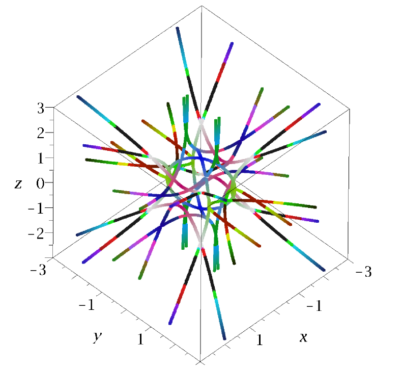
By ApproxPlot (plots:-intersectplot can achieve similar effect).

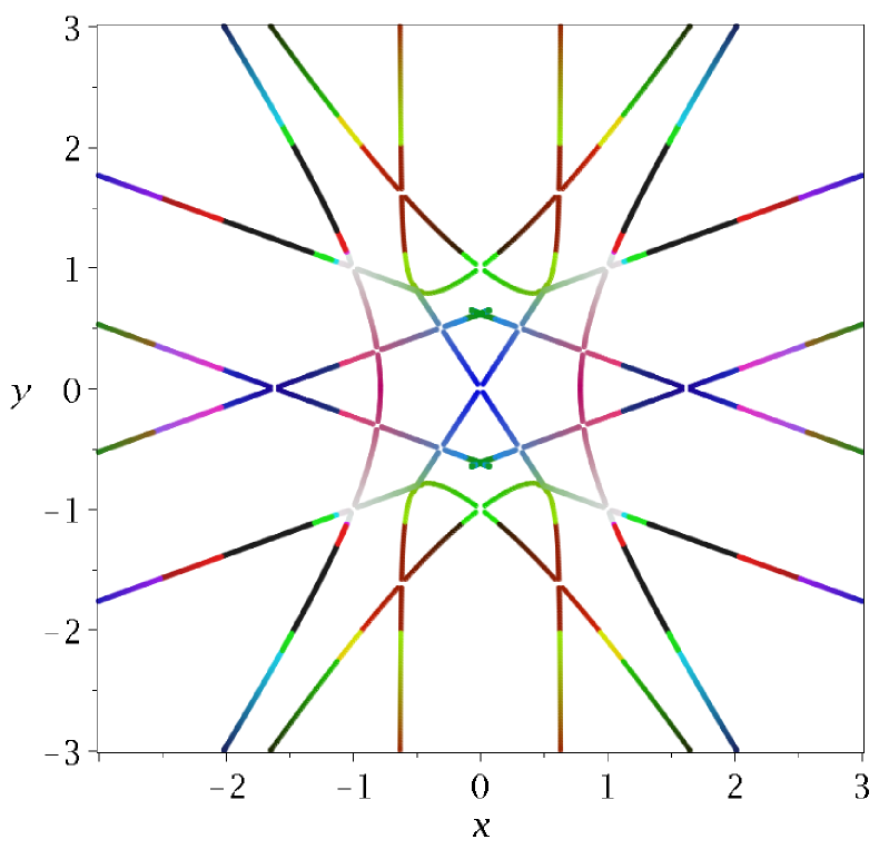
Projection on $(x,y)$ space.

Figure 16: Visualization of Example 5.6.

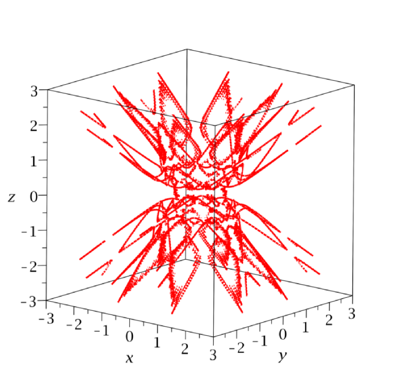
By Maple plots:-intersectplot.

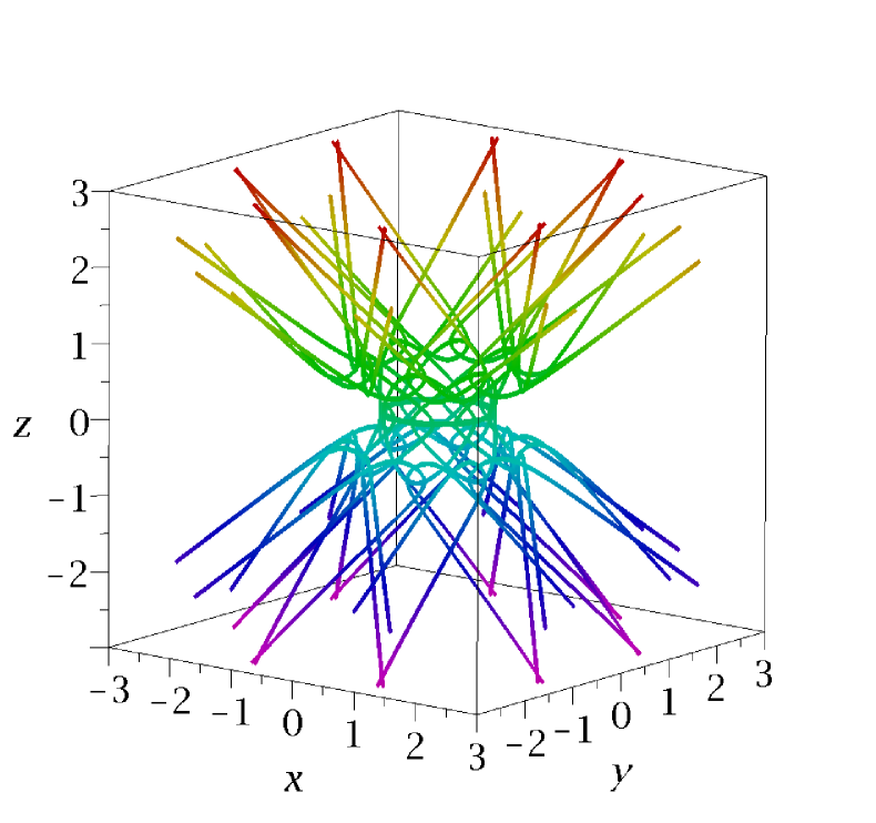
By ApproxPlot.

Figure 17: Visualization of Example 5.7.

6 Conclusion and future work

In this paper, we presented algorithms for visualizing planar and space implicit algebraic curves with singularities. The theoretical algorithm guarantees the polygonal approximation $\varepsilon$-close to the curve. We introduced several strategies to turn the theoretical algorithm to be practical and illustrate its effectiveness by examples. One bottleneck of the algorithm is the computation of singular points, whose efficiency might be improved if the curve is known to be the resultant or discriminant of two polynomials [14].

The algorithm presented in this paper can also be used for tracing space curves with singularities in ambient space with dimension $>3$, which is important for plotting border curves of parametric systems. An efficient algorithm for computing isolated singular points will be important for this method.

From a numeric point of view, singular points are not stable w.r.t. perturbation. A small perturbation may transform a singular point to be exactly nonsingular but still be ill-conditioned in the numerical sense. We proposed heuristic strategies treating these “pseudo-singular” cases and “true-singular” cases in the same away. A limitation of current method is that we assume that the corank of the Jacobian matrix is one. A possible direction to remove such assumptions is to generalize the penalty method for computing witness points in [22] to tracing curves.

- [1] Bresenham J, A linear algorithm for incremental digital display of circular arcs, 1977, Commun. ACM, 20(2):100–106.
- [2] Chandler R, A tracking algorithm for implicitly defined curves, 1988, IEEE Comput. Graph. Appl., 8(2):83–89.
- [3] Hong H, An efficient method for analyzing the topology of plane real algebraic curves, 1996, Mathematics and Computers in Simulation, 42(4):571 – 582.
- [4] Lopes H, Oliveira J, and Figueiredo L, Robust adaptive polygonal approximation of implicit curves, 2002, Computers & Graphics, 26(6):841 – 852.
- [5] Emeliyanenko P, Berberich E, and Sagraloff M, Visualizing arcs of implicit algebraic curves, exactly and fast, Advances in Visual Computing, 2009, 608–619.
- [6] O. Labs, A List of Challenges for Real Algebraic Plane Curve Visualization Software, Nonlinear Computational Geometry, 2010, 137–164.
- [7] Burr M, Choi S, Galehouse B, and Yap C, Complete subdivision algorithms, ii: Isotopic meshing of singular algebraic curves, 2012, Journal of Symbolic Computation, 47(2):131 – 152.
- [8] Jin K, Cheng J, and Gao X, On the topology and visualization of plane algebraic curves, Proceedings of CASC, 2015, 245–259.
- [9] Daouda D, Mourrain B, and Ruatta O, On the computation of the topology of a non-reduced implicit space curve, Proceedings of ISSAC, 2018, 47–54.
- [10] Jin K and Cheng J, Isotopic epsilon-meshing of real algebraic space curves, Proceedings of SNC, 2014, 118–127.
- [11] Stussak C, On reliable visualization algorithms for real algebraic curves and surfaces, PhD thesis, Universitäts- und Landesbibliothek Sachsen-Anhalt, Halle (Saale), 2013.
- [12] Cheng J, Lazard S, Peñaranda L, Pouget M, Rouillier F, and Tsigaridas E, On the topology of real algebraic plane curves, 2010, Mathematics in Computer Science, 4(1):113–137.
- [13] Seidel R and Wolpert N, On the exact computation of the topology of real algebraic curves, Proceedings of the Twenty-first Annual Symposium on Computational Geometry, 2005, 107–115.
- [14] Imbach R, Moroz G, and Pouget M, A certified numerical algorithm for the topology of resultant and discriminant curves, 2017, Journal of Symbolic Computation, 80:285 – 306.
- [15] Gomes A, A continuation algorithm for planar implicit curves with singularities, 2014, Computers & Graphics, 38:365 – 373.
- [16] Brake D, Bates D, Hao W, Hauenstein J, Sommese A, and Wampler C, Algorithm 976: Bertini_real: Numerical decomposition of real algebraic curves and surfaces, 2017, ACM Trans. Math. Softw., 44(1):10:1–10:30.
- [17] Collins G, Quantifier elimination for real closed fields by cylindrical algebraic decompostion, Automata Theory and Formal Languages 2nd GI Conference, 1975, 134–183.
- [18] Rouillier F, Roy M, and Safey El Din M, Finding at least one point in each connected component of a real algebraic set defined by a single equation, 2000, Journal of Complexity, 16(4):716 – 750.
- [19] Chen C, Davenport J, May J, Moreno Maza M, Xia B, Xiao R, Triangular decomposition of semi-algebraic systems, J. Symb. Comp., 49:3–26, 2013.
- [20] Hauenstein J, Numerically computing real points on algebraic sets, 2012, Acta Applicandae Mathematicae, 125(1):105–119.
- [21] Wu W, Reid G, and Feng Y, Computing real witness points of positive dimensional polynomial systems, 2017, Theoretical Computer Science, 681:217 – 231.
- [22] Wu W, Chen C, and Reid G, Penalty function based critical point approach to compute real witness solution points of polynomial systems, Proceeding of CASC, 2017, 377–391.
- [23] Blum L, Cucker F, Shub M, and Smale S, Complexity and Real Computation, Springer-Verlag, New York, 1998.
- [24] Beltrán C and Leykin A, Robust certified numerical homotopy tracking, 2013, Foundations of Computational Mathematics, 13(2):253–295.
- [25] Martin B, Goldsztejn A, Granvilliers L, and Jermann C, Certified parallelotope continuation for one-manifolds, 2013, SIAM Journal on Numerical Analysis, 51(6):3373–3401.
- [26] Yu Y, Yu B, and Dong B, Robust continuation methods for tracing solution curves of parameterized systems, 2014, Numerical Algorithms, 65(4):825–841.
- [27] Bajaj C and Xu G, Piecewise rational approximations of real algebraic curves, 1997, Journal of Computational Mathematics, 15(1):55–71.
- [28] Leykin A, Verschelde J, and Zhao A, Newton’s method with deflation for isolated singularities of polynomial systems, 2006, Theoretical Computer Science, 359(1):111 – 122.
- [29] Chen C, Wu W, and Feng Y, Full rank representation of real algebraic sets and applications, Proceeding of CASC, 2017, 51–65.
- [30] Chen C and Wu W, A numerical method for computing border curves of bi-parametric real polynomial systems and applications, Proceeding of CASC, 2016, 156–171.
- [31] Chen C and Wu W, A numerical method for analyzing the stability of bi-parametric biological systems, Proceeding of SYNASC, 2016, 91–98.
- [32] Yang L and Xia B, Real solution classifications of a class of parametric semi-algebraic systems, Proceeding of A3L, 2005, 281–289.
- [33] Lazard D and Rouillier F, Solving parametric polynomial systems, 2007, J. Symb. Comput., 42(6):636–667.
- [34] Bennett H, Papadopoulou E, and Yap C, Planar minimization diagrams via subdivision with applications to anisotropic voronoi diagrams, 2016, Eurographics Symposium on Geometry Processing, 35(5):229–247.
- [35] Chen C and Wu W, A continuation method for visualizing planar real algebraic curves with singularities, 2018, Proceeding of CASC, 2018, 99–115.
- [36] Wu W and Reid G, Finding points on real solution components and applications to differential polynomial systems. Proceeding of ISSAC, 2013, 339–346.
- [37] Stewart G, Perturbation theory for the singular value decomposition, SVD and Signal Processing, II: Algorithms, Analysis and Applications, 1990, 99–109.
- [38] Shen F, Wu W, and Xia B, Real root isolation of polynomial equations based on hybrid computation, Proceeding of ASCM 2012, 2012, 375–396.
- [39] Lee T, Li T, and Tsai C, Hom4ps-2.0: a software package for solving polynomial systems by the polyhedral homotopy continuation method, 2008, Computing, 83(2):109.
- [40] Duzhin S and Weisstein E, Ordinary double point, From MathWorld–A Wolfram Web Resource.