The turbulent stress spectrum in the inertial and subinertial ranges

Abstract

For velocity and magnetic fields, the turbulent pressure and, more generally, the squared fields such as the components of the turbulent stress tensor, play important roles in astrophysics. For both one and three dimensions, we derive the equations relating the energy spectra of the fields to the spectra of their squares. We solve the resulting integrals numerically and show that for turbulent energy spectra of Kolmogorov type, the spectral slope of the stress spectrum is also of Kolmogorov type. For shallower turbulence spectra, the slope of the stress spectrum quickly approaches that of white noise, regardless of how blue the spectrum of the field is. For fully helical fields, the stress spectrum is elevated by about a factor of two in the subinertial range, while that in the inertial range remains unchanged. We discuss possible implications for understanding the spectrum of primordial gravitational waves from causally generated magnetic fields during cosmological phase transitions in the early universe. We also discuss potential diagnostic applications to the interstellar medium, where polarization and scintillation measurements characterize the square of the magnetic field.

1. Introduction

In aeroacoustics, the stress tensor of the turbulent velocity field plays an important role in sound generation. Its theory goes back to the work of Lighthill (1952a, b), whose equation is also used in astrophysics to describe the heating of stellar coronae by pressure waves excited in the outer convection zones of stars (Stein, 1967). Similarly, in the early universe, the velocity stress and also the combined stress of velocity and magnetic fields can be responsible for driving primordial gravitational waves (Kamionkowski et al., 1994; Durrer et al., 2000). In that case, it is important to relate spectra of the turbulence to the spectra of the kinetic and magnetic stresses in order to compute the spectrum of the gravitational waves (Gogoberidze et al., 2007; Roper Pol et al., 2019).

Empirically, it was known that a velocity or magnetic field with a Kolmogorov-type power law spectrum produces a similar spectrum for the stress, except that in the subinertial range, where the spectral energy increases with wavenumber $k$, the spectral slope of the stress never increases with $k$ faster than for white noise (Roper Pol et al., 2019), even if the turbulence has a blue spectrum. This has important implications for understanding the gravitational wave production at very low frequencies from primordial magnetic fields. Such magnetic fields can be generated at the electroweak phase transition (see Subramanian, 2016, for a review), but their spectrum would be steeper than that of white noise (Durrer & Caprini, 2003) and could not readily explain the shallower white noise spectrum of the stress.

There are different conventions for expressing energy spectra. In this paper, we always present the energy per uniform (linear as opposed to logarithmic) wavenumber interval, so the mean energy density is therefore $\int_{0}^{\infty}E(k)\,{\rm d}k$. In three dimensions, a white noise spectrum is then proportional to $k^{2}$. At some wavenumber $k_{*}$, the spectral energy begins to decline again. The value of $k_{*}$ determines the scale where most of the energy resides. At an even higher wavenumber $k_{\rm D}$, dissipation becomes important and the spectral energy falls off exponentially. The spectral range from $k_{*}$ to $k_{\rm D}$ is called the inertial range. Its spectral slope is determined by the nature of turbulence. For Kolmogorov turbulence, it would be proportional to $k^{-5/3}$. The spectral range below $k_{*}$ is called the subinertial range. Here, the flow tends to be completely uncorrelated, and this is what determines its spectral slope.

In the early universe, when it was just $10^{-11}\,{\rm s}$ old, magnetic fields are believed to have been produced with a blue subinertial range spectrum proportional to $k^{4}$ (Durrer & Caprini, 2003). This is because the magnetic field is divergence free, so the magnetic field itself does not have a white noise spectrum, but it must be the magnetic vector potential that does. Since the magnetic field is the curl of the vector potential, the spectrum of magnetic energy has an extra $k^{2}$ factor as compared to white noise, which is the reason why the magnetic energy spectrum is steeper than that of white noise.

There are other applications where the knowledge of the spectrum of a squared function is important. An example is the magnetic pressure, which can lead to a modulation of the gas pressure and the gas density in the interstellar medium and hence to interstellar scintillation (Lithwick & Goldreich, 2001). Similarly, the square of the magnetic field perpendicular to the line of sight affects dust polarization as well as synchrotron radiation. Both dust and synchrotron emission, as well as interstellar scintillation can provide useful turbulence diagnostics in astrophysics, provided we understand the relationship between the spectra of the magnetic field and its square.

The purpose of the present paper is to derive the relationship between the spectrum of the turbulence and that of the resulting stress. Our calculations are independent of the physical model of the turbulence and apply equally to fluid and magnetohydrodynamic turbulence. With the help of several examples, we illustrate the detailed crossover behavior between different power laws. In all cases, we ignore the temporal evolution of the fluctuations. The temporal correlations are important for the radiation produced by turbulence, e.g., the gravitational waves Gogoberidze et al. (2007), where the turbulent stress tensor enters as a source in the wave equation. Studying this in detail will be the subject of a separate investigation. Here we focus instead on the specific relationships between the spectra of a field and that of its stress found in the numerical simulations of Roper Pol et al. (2019). To illustrate the nature of the problem, it is useful to begin with a simple example of a one-dimensional scalar field and turn then to three-dimensional cases for scalar and vector fields, with and without helicity. The calculations are relatively straightforward, but we are not aware of earlier work addressing this question.

2. A one-dimensional example

Let us consider the fluctuations of a scalar field (e.g., temperature, chemical concentration, etc) $\theta(x)$ as a function of position $x$. We write $\theta(x)$ in terms of its Fourier transform as

$$\theta(x)=\int\tilde{\theta}(k)\,e^{{\rm i}kx}\frac{{\rm d}k}{2\pi}.$$ (1)

Due to spatial homogeneity, the correlation function of the field can be written as

$$\langle\tilde{\theta}(k)\tilde{\theta}^{\ast}(k^{\prime})\rangle=2\pi E(k)\,\delta(k-k^{\prime}),$$ (2)

where $E(k)$ is the energy spectrum of $\theta$. Its Fourier transform yields the two-point correlation function,

$$\langle\theta(x)\theta(x^{\prime})\rangle=\int E(k)\,e^{{\rm i}k(x-x^{\prime})}\frac{{\rm d}k}{2\pi},$$ (3)

and therefore

$$\langle\theta^{2}(x)\rangle=\int E(k)\frac{{\rm d}k}{2\pi}.$$ (4)

Consider now the fluctuations of the squared field

$$\phi(x)=\theta^{2}(x).$$ (5)

We are interested in the two-point correlation function of $\phi(x)$. We now make an important simplifying assumption (for which a physical justification will be provided later) that the four-point correlation function of $\theta$ can be split into two-point correlation functions analogously to the Gaussian rule. We then obtain

$$\langle\phi(x)\phi(x^{\prime})\rangle=\langle\theta^{2}\rangle^{2}+2\langle\theta(x)\theta(x^{\prime})\rangle^{2}.$$ (6)

In order to find the energy spectrum of $\phi$, we Fourier transform Equation (6) to obtain

$$\langle\phi(x)\phi(x^{\prime})\rangle=\int F(k)e^{{\rm i}k(x-x^{\prime})}\frac{{\rm d}k}{2\pi},$$ (7)

where

$$F(k)=2\pi\langle\theta^{2}\rangle^{2}\delta(k)+2\int E(k-k^{\prime})E(k^{\prime})\frac{{\rm d}k^{\prime}}{2\pi}.$$ (8)

The first term could be removed by subtracting the average of $\langle\theta^{2}\rangle^{2}$.

Let us assume we know the spectrum $E(k)$. Our question concerns the resulting spectrum $F(k)$. Specifically, we may think of a piece-wise power law of the form $E(k)\propto k^{\alpha}$, where $\alpha$ is positive for $0<k<k_{*}$, and negative for $k_{*}\leq k\leq k_{\rm D}$, so that the energy is contained mostly at the scale $k_{*}^{-1}$, which is the outer scale of fluctuations. We expect $F(k)$ to be asymptotically also of piecewise power law form, $F(k)\propto k^{\beta}$ within a certain $k$-range. For $k>0$ we have

$$F(k)=2\int_{-\infty}^{\infty}E(k^{\prime})\,E(k-k^{\prime})\,\frac{{\rm d}k^{\prime}}{2\pi},$$ (9)

where we have highlighted the fact that the integration over $k^{\prime}$ goes from $-\infty$ to $+\infty$.

At small wavenumbers $k\ll k_{*}$, the integral in Equation (9) is dominated by the scales $k^{\prime}$ comparable to the outer scale $k_{*}$, so we may expand

$$E(k^{\prime}-k)\approx E(k^{\prime})-k\frac{{\rm d}E(k^{\prime})}{{\rm d}k^{\prime}}+\frac{1}{2}k^{2}\frac{{\rm d}^{2}E(k^{\prime})}{{\rm d}k^{\prime 2}}.$$ (10)

We then obtain from Equation (9) the asymptotic behavior of $F(k)$ at small wavenumbers as $F(k)\approx c_{1}-c_{2}k^{2}$, where $c_{1}$ and $c_{2}$ are positive constants. This means that the spectrum $F(k)$ is flat at small $k$, that is, $\beta=0$.

In order to find the asymptotic behavior at large wavenumbers, $k\gg k_{1}$, we note that, if the energy spectrum in this interval is $E(k)\propto k^{\alpha}$, and $-3<\alpha<-1$, then the correlation function of $\theta$ behaves at small scales as

$$\frac{\langle\theta(x)\theta(x^{\prime})\rangle}{\langle\theta^{2}\rangle}\approx 1-\left|\frac{x-x^{\prime}}{L}\right|^{-\alpha-1},$$ (11)

where $L\sim 1/k_{1}$ is a scale comparable to the outer scale of the fluctuations. The square of this correlation function then scales as

$$\frac{\langle\theta(x)\theta(x^{\prime})\rangle^{2}}{\langle\theta^{2}\rangle^{2}}\approx 1-2\left|\frac{x-x^{\prime}}{L}\right|^{-\alpha-1},$$ (12)

where we have expanded the right-hand side in the small parameter $|x-x^{\prime}|/L$. Therefore, asymptotically at large $k$, the spectrum $F(k)\sim k^{\beta}$ should scale with the same scaling exponent as the original energy spectrum $E(k)$, that is, $\beta=\alpha$.

Expressions (11) and (12) allow us to provide a physical motivation for splitting the fourth-order correlation functions of $\theta$ in the pair-wise ones in formula (6). For that, consider the Fourier component of the $\phi$ field,

$$\phi(k)=\int\tilde{\theta}(k^{\prime})\tilde{\theta}(k-k^{\prime})\frac{{\rm d}k^{\prime}}{2\pi}.$$ (13)

One can ask what typical wavenumbers $k^{\prime}$ and $k-k^{\prime}$ contribute to this integral. The first possibility would be to have both wavenumbers of the same order, $k^{\prime}\sim k-k^{\prime}\sim k/2$. The second possibility is to have one of these numbers much larger than the other one, say $k^{\prime}\approx k$ and $k-k^{\prime}\approx 0$. Since for the Kolmogorov spectrum, the intensity of fluctuations declines rapidly with wavenumber, the dominant contribution is expected to come from the second possibility. This means that the fluctuating fields $\tilde{\theta}(k)$ contributing to the integral (13) have rather disparate wavenumbers. Since the assumption of locality of Kolmogorov turbulence implies that the small-scale fluctuations are uncorrelated from the large-scale ones, we may average the $\tilde{\theta}$ fields in $\phi$ independently, which formally leads to the “Gaussian splitting rule” resulting in Equation (6).

To illustrate the resulting slope of $F(k)$ for given $E(k)$, we consider as a first example

$$E(k)=\left\{\!\!\begin{array}[]{ll}&k^{-2}\quad\mbox{for $1\leq k\leq 100$},\\ &0\quad\quad\mbox{otherwise}.\end{array}\right.$$ (14)

We compute the convolution in Equation (9) through multiplication of the Fourier transformed quantities, i.e., through their autocorrelation function,

$$\tilde{F}(x)=|\tilde{E}(x)|^{2},$$ (15)

where $\tilde{E}(x)=\int e^{{\rm i}kx}E(k)\,{\rm d}k/2\pi$, and likewise for $\tilde{F}(x)$. Note that the Fourier integral is carried out from $-\infty$ to $+\infty$ and that $E(k)$ is symmetric about $k=0$. We evaluate the integral in Equation (9) numerically. The energy-carrying wavenumber in our example is $k_{*}\equiv 1$.

The result is plotted in Figure 1. We see that in the range $5<k<100$, we have $F(k)\approx E(k)$. At $k=2$, the profile of $F(k)$ has a sharp dip, which results in a local maximum at $k\approx 3$, before approaching $E(k)$. At small values of $k$, however, $F(k)$ always has a flat spectrum.

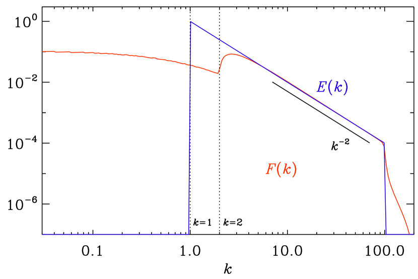
Figure 1.— Numerically computed $F(k)$ (red) for $E(k)=k^{-2}$ (blue) for $1\leq k\leq 100$ (and zero otherwise). The vertical solid and dotted lines mark $k=1$ and $2$, respectively.

In our second example, we define the spectrum as

$$E(k)=\frac{|k|^{\alpha_{1}}}{[1+|k|^{(\alpha_{1}-\alpha_{2})q}]^{1/q}}e^{-(|k|/k_{\rm D})^{2}},$$ (16)

where we allow for an exponential cutoff at the dissipation wavenumber $k_{\rm D}=100$ and a power law subinertial range of the form $k^{\alpha_{1}}$ with $\alpha_{1}=10$, $4$, $2$, $1$, and $0$. Here we have included the exponents $q$ and $1/q$ with $q=4$ to sharpen the cross-over between the subinertial range and the inertial range power laws. Furthermore, $\alpha_{2}=-5/3$ is the exponent chosen for the Kolmogorov-type inertial range.

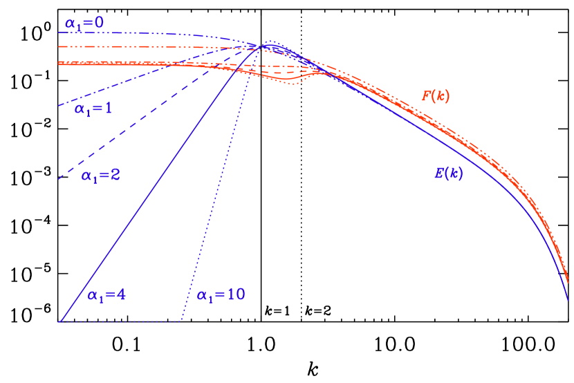
Figure 2.— Similar to Figure 1, but for different subinertial range slopes: $\alpha_{1}=0$ (triple-dot-dashed), $1$ (dot-dashed), $2$ (dashed), $4$ (solid), and $10$ (dotted).

The result is plotted in Figure 2. In all these cases, we see that $F(k)$ has a flat spectrum for $k\lesssim 0.5$. We see that the dip at $k=2$ has disappeared for $\alpha_{1}=0$, but it becomes stronger when $\alpha_{1}$ is large and $\beta_{1}$ develops a white noise spectrum for small $k$.

3. The three-dimensional case

Next, we consider fully three-dimensional examples. In the case of a scalar field, $\theta(\bm{r})$, the derivation is similar to the one-dimensional case. The Fourier transform of the field is defined as

$$\theta(\bm{r})=\int\tilde{\theta}(\bm{k})e^{{\rm i}\bm{k}\cdot\bm{r}}\frac{{\rm d}^{3}k}{(2\pi)^{3}}.$$ (17)

Then, given the correlation function of the fields

$$\langle\tilde{\theta}(\bm{k})\tilde{\theta}^{*}(\bm{k}^{\prime})\rangle=(2\pi)^{3}I(\bm{k})\delta(\bm{k}-\bm{k}^{\prime}),$$ (18)

one derives the correlation function of the quadratic field $\phi(\bm{r})=\theta^{2}(\bm{r})$ in the form

$$\langle\phi(\bm{r})\phi(\bm{r}^{\prime})\rangle=\int H(\bm{k})\frac{{\rm d}^{3}k}{(2\pi)^{3}},$$ (19)

where

$$H(\bm{k})=(2\pi)^{3}\langle\theta^{2}\rangle^{2}\delta(\bm{k})+2\int\!I(\bm{k}^{\prime})I(\bm{k}-\bm{k}^{\prime})\frac{{\rm d}^{3}k^{\prime}}{(2\pi)^{3}}.\quad$$ (20)

3.1. Nonhelical vector fields

The situation is qualitatively similar for a vector field. Let us consider an incompressible vector field $\bm{u}(\bm{r})$, representing a velocity or magnetic field. Its Fourier transform is defined as

$$\bm{u}(\bm{r})=\int\tilde{\bm{u}}(\bm{k})\,e^{{\rm i}\bm{k}\cdot\bm{r}}\frac{{\rm d}^{3}k}{(2\pi)^{3}}.$$ (21)

We assume that the distribution of this field is homogeneous and isotropic, so that its correlation function is given by

$$\langle\tilde{u}^{i}(\bm{k})\tilde{u}^{*j}(\bm{k}^{\prime})\rangle=(2\pi)^{3}I(\bm{k})\delta(\bm{k}-\bm{k}^{\prime})P_{ij}(\bm{k}),$$ (22)

where we have denoted $P_{ij}(\bm{k})=\delta_{ij}-k_{i}k_{j}/k^{2}$. The energy of this field then satisfies

$$\langle u^{2}(\bm{r})\rangle=\int 2I(\bm{k})\frac{{\rm d}^{3}k}{(2\pi^{3})}.$$ (23)

Similarly to the one-dimensional case, we are interested in the correlation function of the quadratic field $\phi^{ij}({\bf r})=u^{i}(\bm{r})u^{j}(\bm{r})$. Assuming that the four-point correlation functions of the $u$-field can be split into the two-point ones by using the Gaussian rule, we get

$$\langle\phi^{ij}(\bm{k})\phi^{*lm}(\tilde{\bm{k}})\rangle=$$

$$\delta(\bm{k})\delta(\tilde{\bm{k}})\int I(\bm{k}^{\prime})I(\bm{k}^{\prime\prime})P_{ij}(\bm{k}^{\prime})P_{lm}({\bf k}^{\prime\prime}){\rm d}^{3}k^{\prime}{\rm d}^{3}k^{\prime\prime}+$$

$$\delta(\bm{k}-{\tilde{\bm{k}}})\int I(\bm{k}-\bm{k}^{\prime})I(\bm{k}^{\prime})P_{il}(\bm{k}-\bm{k}^{\prime})P_{jm}(\bm{k}^{\prime}){\rm d}^{3}k^{\prime}+$$

$$\delta(\bm{k}-{\tilde{\bm{k}}})\int I(\bm{k}-\bm{k}^{\prime})I(\bm{k}^{\prime})P_{im}(\bm{k}-\bm{k}^{\prime})P_{jl}(\bm{k}^{\prime}){\rm d}^{3}k^{\prime}.\quad$$ (24)

As an example, consider the correlation function of energy fluctuations,

$$\frac{\langle\phi^{ii}(\bm{k})\phi^{*ll}(\tilde{\bm{k}})\rangle}{(2\pi)^{3}}=\delta(\bm{k})\langle u(\bm{r})^{2}\rangle^{2}+2\delta(\bm{k}-\tilde{\bm{k}})H(\bm{k}),\;$$ (25)

where

$$H(\bm{k})=\int I(\bm{k}^{\prime})I(\bm{k}-\bm{k}^{\prime})\left[1+\frac{[\bm{k}^{\prime}\cdot(\bm{k}-\bm{k}^{\prime})]^{2}}{k^{\prime 2}(\bm{k}-\bm{k}^{\prime})^{2}}\right]\!\frac{{\rm d}^{3}k^{\prime}}{(2\pi)^{3}}.$$ (26)

In a statistically isotropic case, instead of the power spectrum $I({k})$, it is convenient to use the energy spectrum $E({k})=4\pi k^{2}I({k})$, and similarly $F(k)=4\pi k^{2}H(k)$. The above equation then becomes

$$F(k)=\int E(k^{\prime})E(\kappa)\frac{k^{2}}{\kappa^{2}}\left[1+\frac{(k\mu-k^{\prime})^{2}}{\kappa^{2}}\right]\frac{{\rm d}k^{\prime}\,{\rm d}\mu}{(2\pi)^{3}},$$ (27)

where

$$\kappa=|\bm{k}-\bm{k}^{\prime}|=\sqrt{k^{2}+k^{\prime 2}-2kk^{\prime}\mu},$$ (28)

and $\mu=\bm{k}\cdot\bm{k}^{\prime}/kk^{\prime}$ is the cosine of the angle between $\bm{k}$ and $\bm{k}^{\prime}$.

3.2. Helical vector fields

For completeness, we also consider a more general case, when the system is not mirror invariant. In this case, the field correlation function has an extra term,

$$\langle\tilde{u}^{i}(\bm{k})\tilde{u}^{*j}(\bm{k}^{\prime})\rangle=(2\pi)^{3}I(k)\delta(\bm{k}-\bm{k}^{\prime})P_{ij}(\bm{k})$$

$$-(2\pi)^{3}J(k)\delta(\bm{k}-\bm{k}^{\prime})\epsilon_{ijl}{\rm i}k^{l}/k.$$ (29)

The last term in this expression is responsible for the helicity of the field. In particular, it enters the helicity integral

$$\int\langle(\bm{\nabla}\times\bm{u})\cdot\bm{u}\rangle\,{\rm d}^{3}x=2\int k\,J(k)\frac{{\rm d}^{3}k}{(2\pi)^{3}},$$ (30)

which would be zero in a mirror-invariant case. The helicity spectral function $J(k)$ is not necessarily positive, but it has to satisfy the realizability condition $|J(k)|\leq I(k)$. The generalization of our results to the helical case is straightforward; it is achieved by replacing the non-helical terms $I(k)P_{ij}({\bf k})$ in Eq. (3.1) by their helical counterparts $I(k)P_{ij}({\bf k})-J(k)\epsilon_{ijl}{\rm i}k^{l}/k$. For example, in the correlation function of the energy fluctuations (25) we will need to replace the $H({\bf k})$ function (26) by the general expression

$$H(\bm{k})=\int I(\bm{k}^{\prime})I(\bm{k}-\bm{k}^{\prime})\left[1+\frac{[\bm{k}^{\prime}\cdot(\bm{k}-\bm{k}^{\prime})]^{2}}{k^{\prime 2}(\bm{k}-\bm{k}^{\prime})^{2}}\right]\!\frac{{\rm d}^{3}k^{\prime}}{(2\pi)^{3}}$$

$$-2\int J(\bm{k}^{\prime})J(\bm{k}-\bm{k}^{\prime})\left[\frac{\bm{k}^{\prime}\cdot(\bm{k}-\bm{k}^{\prime})}{k^{\prime}|\bm{k}-\bm{k}^{\prime}|}\right]\!\frac{{\rm d}^{3}k^{\prime}}{(2\pi)^{3}}.\quad\quad$$ (31)

Again, in a statistically isotropic case, instead of the power spectrum $J({k})$, it is convenient to introduce the helicity spectrum defined as $G({k})=4\pi k^{2}J({k})$. The above equation then becomes

$$F(k) = \int E(k^{\prime})E(\kappa)\,\frac{k^{2}}{\kappa^{2}}\left[1+\frac{(k\mu-k^{\prime})^{2}}{\kappa^{2}}\right]\!\frac{{\rm d}k^{\prime}\,{\rm d}\mu}{(2\pi)^{3}}$$ (32)

$$-2\int G(k^{\prime})G(\kappa)\,\frac{k^{2}}{\kappa^{2}}\,\frac{k\mu-k^{\prime}}{\kappa}\,\frac{{\rm d}k^{\prime}\,{\rm d}\mu}{(2\pi)^{3}}.$$

which can readily be evaluated using numerical integration.

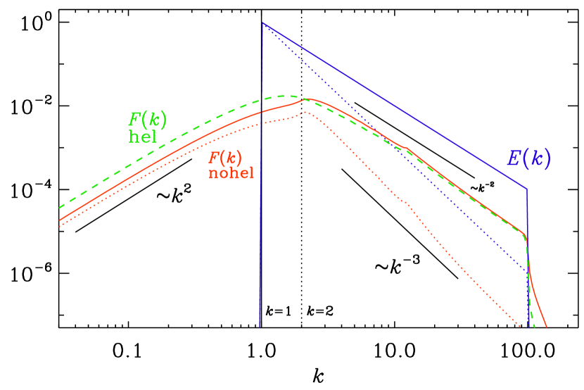
Figure 3.— Similar to Figure 1, but for the 3D integral for power laws $k^{\alpha}$ in $1<k<100$ with $\alpha=-2$ and $-3$. For $\alpha=-2$, $F(k)$ is also plotted for the helical case (green dashed line).

3.3. Examples

In Figure 3, we show the results for the case of a single power low, as in Equation (12). We consider two values for the slope $\alpha$ ($-2$ and $-3$) in the range $1\leq k\leq 100$. We see that, for $k>2$, we obtain for $F(k)$ a power law, $F(k)\propto k^{\beta}$, with $\beta=\alpha$, as in the one-dimensional case. In the range $1<k<2$, $F(k)$ is still increasing with $k$, but the slope is slightly less steep than two. We emphasize that this behavior is different from that in the one-dimensional case, where we saw instead a marked dip in $F(k)$.

In Figure 3, we also plot $F(k)$ for the case of a fully helical field using Equation (32), where $G(k)=E(k)$ is assumed. We see that the basic features of $F(k)$ are rather similar to the case without helicity, but there is now slightly more power in the subinertial range, where $F(k)$ appears to be elevated by about a factor of two. In the inertial range, on the other hand, $F(k)$ is not affected by the presence of helicity.

Next, we consider a spectrum with two different slopes, $\alpha_{1}$ and $\alpha_{2}$, along with an exponential cutoff, just as in Equation (16). Again, we denote the corresponding slopes of $F(k)$ as $\beta_{1}$ and $\beta_{2}$, respectively. Here, we always assume a Kolmogorov inertial range spectrum for $E(k)$, i.e., $\alpha_{2}=-5/3$, and we vary $\alpha_{1}$ from $0$ to $10$. Physically relevant are the Saffman ($\alpha_{1}=2$) and Batchelor ($\alpha_{1}=4$) asymptotic scalings for $k\to 0$ (e.g., Davidson, 2015). In our finite simulation domain it is, however, interesting to consider arbitrary values of $\alpha_{1}$.

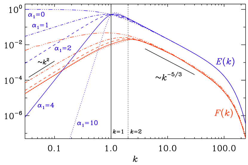
Figure 4.— Similar to Figure 2, but now for the three-dimensional case. Blue: $E(k)$, red: $F(k)$, for $\alpha_{1}=0$ (triple-dot-dashed), $1$ (dot-dashed), $2$ (dashed), $4$ (solid), and $10$ (dotted).

Figure 4 confirms the statement of Roper Pol et al. (2019) that $\beta=2$ is obtained even if $E(k)$ has a blue spectrum, i.e., $\alpha\geq 2$. We also see from Figure 4 that for $\alpha_{1}=2$, the crossover from the $k^{2}$ scaling for small $k$ to the $k^{-5/3}$ scaling for large $k$ extends now over more than one decade ($0.2<k<5$). This shows that we may expect slight differences when approximate scalings are based on the inspection of spectra over a limited dynamical range.

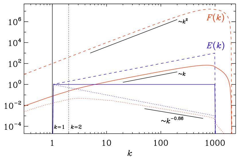
Figure 5.— Solutions of the 3D integral for power laws $k^{\alpha}$ in $1<k<1000$ with $\alpha=-1$, 0, and 1.

Figure 6.— $\beta$ versus $\alpha$ in the range from $-2$ to $2$ for one-dimensional (1D) and three-dimensional (3D) cases. The dotted line indicates the diagonal.

To study in more detail the crossover from $\beta=2$ for $\alpha\geq 2$ to $\beta=\alpha$ for $\alpha$ of around and below $-5/3$, for example, let us now consider single power law spectra within a more extended range $1\leq k\leq 1000$ using intermediate values $\alpha=-1$, 0, and 1. No distinction between $\alpha_{1}$ and $\alpha_{2}$ will therefore be made. The result is shown in Figure 5. We see that in this range of $\alpha$, $\beta$ is always larger than $\alpha$. We see that already for the scale-invariant $k^{-1}$ spectrum, we have $\beta=-0.86$, so the $\beta=\alpha$ relation is only approximately obeyed.

To determine the relation between $\alpha$ and $\beta$ in the intermediate regime, we now compute $\beta$ using the same numerical setup as before, but we now consider power law scalings in a range that is 100 times larger, $1\leq k\leq 10^{5}$. The result is shown in Figure 6. Here we also compare with the corresponding results in one dimension. We now see that in the range $-1<\alpha<1$, the value of $\beta$ deviates markedly from the $\beta=\alpha$ relation, and that we have $\beta\approx 2$ already for $\alpha=1$.

Likewise in one dimension, the $\beta=\alpha$ relation is only true for $\alpha<-1$. Again, there is a small intermediate interval, $-1<\alpha<0$, where $\beta$ is somewhat larger than $\alpha$, but this departure is by far not as dramatic as in three dimensions; see Figure 6.

4. Comparison with turbulence simulations

To address the assumption of Gaussianity, we now present the results of numerical simulations of the hydromagnetic equations for a weakly compressible gas in a cubic domain of size $L^{3}$ using $1024^{3}$ mesh points. We employ the Pencil Code, which uses sixth order accurate finite differences for the spatial discretization and a third order time stepping scheme. We first consider decaying nonhelical turbulence. Our simulations are similar to Run A of Brandenburg et al. (2017), where $\alpha_{1}\approx 4$ and $\alpha_{2}\approx-5/3$. The turbulence is magnetically dominated, so the velocity is almost entirely the result of the Lorentz force.

In Figure 7, we present the results for the magnetic energy spectrum $E_{\rm M}(k)$ after about 100 Alfvén times. Initially, the peak of $E_{\rm M}(k)$ was at $k=k_{*}$ with $k_{*}L/2\pi=60$, but, owing to an effect similar to the inverse cascade—here without helicity—the peak has moved to about $k_{*}L/2\pi=15$ by the end of the simulation; see Brandenburg et al. (2015) for similar results. In Figure 7 we also compare with the corresponding spectrum of $\bm{B}^{2}$, referred to as $F_{i}(k)$, where $i={\rm M}$ stands for the magnetic stress. We see that the spectral slopes of $E_{\rm M}$ and $F_{\rm M}$ agree in the inertial range. In the subinertial range, the slopes of $E_{\rm M}$ and $F_{\rm M}$ are, as expected, different from each other. However, the values of the slopes, 3.5 and 1.5, respectively, are below the expectations of 4 and 2, respectively.

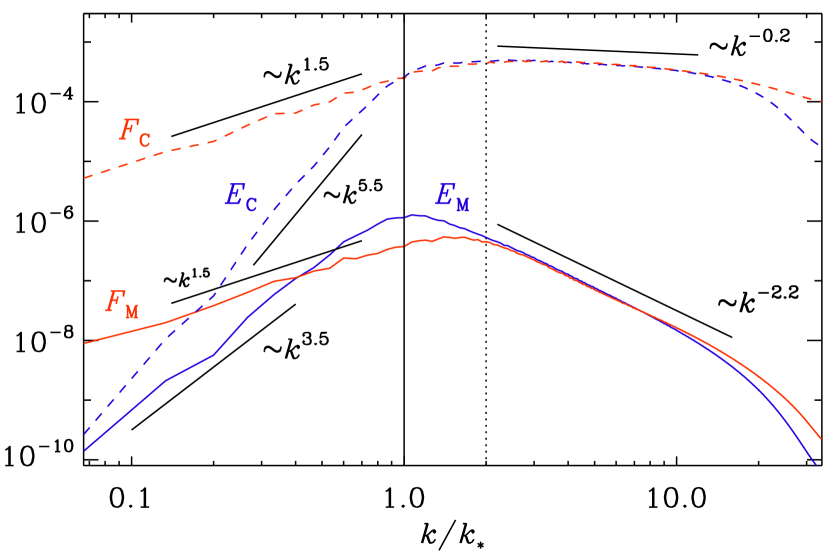
Figure 7.— Comparison with $E_{i}(k)$ and $F_{i}(k)$ from a turbulence simulations for the magnetic field ($i={\rm M}$) and the current density ($i={\rm C}$). The $F_{i}(k)$ spectra have been shifted to show the agreement of their slopes with those of $E_{i}(k)$ for large $k$.

To characterize the departure from Gaussianity, we have computed the kurtosis of the magnetic field separately for all three components and then take the average, which is denoted by

$$\mbox{kurt}\bm{B}=-3+\frac{1}{3}\sum_{i=1}^{3}\langle B_{i}^{4}\rangle/\langle B_{i}^{2}\rangle^{2}.$$ (33)

We find a rather small value of less than 0.1. Thus, the field is close to Gaussian and our results are qualitatively in close agreement with those of the present paper.

To compare with a field where the assumption of Gaussianity cannot be justified, we also show the results for the normalized current density $\bm{J}=\bm{\nabla}\times\bm{B}$. We denote the corresponding spectra for current density by $E_{i}(k)$ and $F_{i}(k)$ with $i={\rm C}$. The kurtosis of $\bm{J}$, defined analogous to $\mbox{kurt}\bm{B}$, is about 4.5.

In the inertial range, $E_{\rm M}$ has a slope of about $-2.2$, which is steeper than that of the Kolmogorov spectrum. The current density spectrum has a slope of about $-0.2$. The slopes were initially closer to the Kolmogorov values, but they became steeper with time. What is important, however, is that in the inertial range, the spectral slopes of $F_{\rm M}$ and $F_{\rm C}$ agree with those of $E_{\rm M}$ and $E_{\rm C}$, respectively, i.e., both have slopes of $-2.2$ and $-0.2$, respectively. In the subinertial range, the slopes are again somewhat different from the expectation. We find $\alpha_{1}=3.5$ and $5.5$ for the spectra of $E_{\rm M}$ and $E_{\rm C}$, respectively, but $1.5$ for the slopes of both $F_{\rm M}$ and $F_{\rm C}$. It should be noted that, even under the assumption of isotropy, the stress tensor contains different contributions (scalar, vector, and tensor modes) that might behave differently. However, the resulting differences are also sensitive to the nature of the turbulence, whose study is beyond the scope of the present paper.

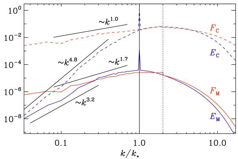
Figure 8.— Similar to Figure 7, but for forced turbulence with $k_{*}=30$.

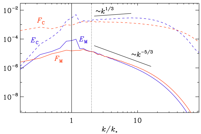
Figure 9.— Similar to Figure 7, but for forced turbulence with $k_{*}=6$.

Next, we compare with two runs of forced turbulence. In these two examples, we consider the forcing wavenumbers $k_{*}=30$ and $6$, respectively. In the former case (Figure 8), the subinertial range is more developed. The magnetic field and current density are now closer to being Gaussian ($|\mbox{kurt}\bm{B}|\lesssim 0.1$ and $\mbox{kurt}\bm{J}\approx 1.4$). We see that in the subinertial range, the slope of $F_{\rm C}$ is now even more shallow ($\beta_{1}=1$), while that of $F_{\rm M}$ is slightly steeper ($\beta_{1}=1.7$), but still not quite as steep as what is expected ($\beta_{1}=2$).

In the latter run with $k_{*}=6$ (Figure 9), the inertial range is more developed and we see a clear $k^{-5/3}$ spectrum in $E_{\rm M}$. The magnetic field and current density are now further away from being Gaussian ($\mbox{kurt}\bm{B}=0.1...0.2$ and $\mbox{kurt}\bm{J}\approx 5$). In the inertial range, the slope for $E_{\rm C}$ agrees with what is expected for Kolmogorov-type turbulence ($1/3$ for $F_{\rm M}$). However, we also see departures from the $\beta=\alpha$ relation, where the $\beta$ for $F_{\rm M}$ is slightly larger, while that of $F_{\rm C}$ is now smaller and even negative.

5. Conclusions

We have derived the general formula that allows us to compute a spectrum $F(k)$ of the square of a fluctuating field whose spectrum, in turn, is $E(k)$. Our results are independent of whether the spectrum is that of a scalar or that of a vector field. We have seen that in the inertial range with $E(k)\propto k^{\alpha}$ and $\alpha\lesssim-1$, we find a spectrum $F(k)\propto k^{\beta}$ with $\beta\approx\alpha$ if we are sufficiently far away from the boundaries of the validity range of where the power law applies. In the subinertial range, where $\alpha\gtrsim 1$, we find $\beta\approx 2$.

A possible application of our work concerns the generation of gravitational waves from hydrodynamic and hydromagnetic turbulence with a known energy spectrum $E(k)$. The resulting stress $T_{ij}$ sources a wave equation of the form $\Box h_{ij}=T_{ij}$, where, except for normalization factors, $h_{ij}$ is the linearized strain field, $\Box=\nabla^{2}-c^{-2}\partial^{2}/\partial t^{2}$ is the d’Alembertian wave operator, and $c$ is the speed of light. The actual gravitational wave fields are the transverse and traceless projections of $h_{ij}$. The nature of the wave operator can lead to a complicated relation between the spectra of $h_{ij}$ and $T_{ij}$ (e.g., Roper Pol et al., 2020). If, however, the time delay in the wave equation can be neglected, the spectrum of $h_{ij}$ is proportional to $F(k)/k^{4}$.

The simulations of Roper Pol et al. (2020) show that most of the wave generation occurs at the time when the stress has reached maximum amplitude. Subsequent changes of the source hardly contribute to wave production. It may be for this reason that the assumption of no time delay is a reasonable one. Under this assumption, we expect that the gravitational wave energy, which is proportional to $(\partial h_{ij}/\partial t)^{2}$, should be proportional to $F(k)/k^{2}$; see Roper Pol et al. (2020) for details. The extent of the empirically determined departures from this simplistic way of estimating the gravitational wave energy spectrum are not yet fully understood and would need to be determined numerically or analytically, similarly to earlier work using the aeroacoustic approximation of Lighthill (1952a), as already done by Gogoberidze et al. (2007) in the context of primordial gravitational waves.

Cosmological magnetic fields may well be helical (Tashiro et al., 2014). They could be generated by the chiral magnetic effect (Joyce & Shaposhnikov, 1997; Boyarsky et al., 2012; Yamamoto, 2016; Anand et al., 2017). However, even under the most optimistic conditions, this effect can only produce about $10^{-18}\,{\rm G}$ on a scale of $1\,{\rm Mpc}$ at the present time (Brandenburg et al., 2017). Our work now shows that the presence of magnetic helicity enhances the stress spectrum by up to a factor of two in the subinertial range, while leaving that in the initial range unchanged. This implies a small shift in the peak of the stress spectrum, which itself would hardly be a distinguishing feature. However, helical magnetic fields lead to circular polarization of gravitational waves (Kahniashvili et al., 2005), which may be detectable with the Laser Interferometer Space Antenna if there is a sufficiently strong dipolar anisotropy in the signal (Domcke et al., 2019).

Another potentially important application concerns the spectrum of the parity even and parity odd linear polarization modes. Those depend quadratically on the magnetic field components perpendicular to the line of sight (Caldwell et al., 2017; Kandel et al., 2017; Brandenburg et al., 2019). Our work now suggests that, measuring the polarization spectrum, one can only infer the spectrum of the underlying turbulence if $\alpha<-1$.

References

- Anand et al. (2017) Anand, S., Bhatt, J. R., & Pandey, A. K. 2017, JCAP, 07, 051
- Boyarsky et al. (2012) Boyarsky, A., Fröhlich, J., & Ruchayskiy, O. 2012, PhRvL, 108, 031301
- Brandenburg et al. (2019) Brandenburg, A., Bracco, A., Kahniashvili, T., Mandal, S., Roper Pol, A., Petrie, G. J. D., & Singh, N. K. 2019, ApJ, 870, 87
- Brandenburg et al. (2017) Brandenburg, A., Kahniashvili, T., Mandal, S., Roper Pol, A., Tevzadze, A. G., & Vachaspati, T. 2017, PhRvD, 96, 123528
- Brandenburg et al. (2015) Brandenburg, A., Kahniashvili, T., & Tevzadze, A. G. 2015, PhRvL, 114, 075001
- Brandenburg et al. (2017) Brandenburg, A., Schober, J., Rogachevskii, I., Kahniashvili, T., Boyarsky, A., Fröhlich, J., Ruchayskiy, O., & Kleeorin, N. 2017, ApJL, 845, L21
- Caldwell et al. (2017) Caldwell, R. R., Hirata, C., & Kamionkowski, M. 2017, ApJ, 839, 91
- Davidson (2015) Davidson, P. A. 2015, Turbulence: An introduction for scientists and engineers (Oxford: Oxford University Press)
- Domcke et al. (2019) Domcke, V., Garcia-Bellido, J., Peloso, M., Pieroni, M., Ricciardone, A., Sorbo, L., & Tasinato, G. 2019, arXiv:1910.08052.
- Durrer et al. (2000) Durrer, R., Ferreira, P. G., & Kahniashvili, T. 2000, PhRvD, 61, 043001
- Durrer & Caprini (2003) Durrer, R., and Caprini, C. 2003, J. Cosmol. Astropart. Phys., 0311, 010
- Gogoberidze et al. (2007) Gogoberidze, G., Kahniashvili, T. and Kosowsky, A. 2007, PhRvD, 76, 083002
- Joyce & Shaposhnikov (1997) Joyce, M., & Shaposhnikov, M. 1997, PhRvL, 79, 1193
- Kahniashvili et al. (2005) Kahniashvili, T., Gogoberidze, G., & Ratra, B. 2005, PhRvL, 95, 151301
- Kamionkowski et al. (1994) Kamionkowski, M., Kosowsky, A., & Turner, M. 1994, PhRvD, 49, 2837
- Kandel et al. (2017) Kandel, D., Lazarian, A., & Pogosyan, D. 2017, MNRAS, 472, L10
- Lighthill (1952a) Lighthill, M. J. 1952a, Proc. Roy. Soc. Lond. A, 211, 564
- Lighthill (1952b) Lighthill, M. J. 1952b, Proc. Roy. Soc. Lond. A, 222, 1
- Lithwick & Goldreich (2001) Lithwick, Y., & Goldreich, P. 2001, ApJ, 562, 279
- Roper Pol et al. (2020) Roper Pol, A., Brandenburg, A., Kahniashvili, T., Kosowsky, A., & Mandal, S. 2020, GApFD, 114, 130
- Roper Pol et al. (2019) Roper Pol, A., Mandal, S., Brandenburg, A., Kahniashvili, T., & Kosowsky, A. 2019, PhRvD, submitted, arXiv:1903.08585.
- Stein (1967) Stein, R. F. 1967, SoPh, 2, 385
- Subramanian (2016) Subramanian, K. 2016, RPPh, 79, 076901
- Tashiro et al. (2014) Tashiro, H., Chen, W., Ferrer, F., & Vachaspati, T. 2014, MNRAS, 445, L41
- Yamamoto (2016) Yamamoto, N. 2016, PhRvD, 93, 125016