Performance and error modeling of Deutsch’s algorithm in IBM Q

Abstract

The performance of quantum computers today can be studied by analyzing the effect of errors in the result of simple quantum algorithms. The modeling and characterization of these errors is relevant to correct them, for example, with quantum correcting codes. In this article we characterize the error of the five qubits quantum computer ibmqx4 (IBM Q), using a Deutsch algorithm and modeling the error by Generalized Amplitude Damping (GAD) and a unitary misalignment operation.

I Introduction

The idea of using the quantum mechanics as a calculation tool arose from the pioneering works of Feynman and Deutsch Feynman_82 ; Deutsch_85 in the 80s. It is based on the use of properties as superposition and entanglement for the realization of computational task. This requires a quantum computer that works at the microscopic level. This way, a quantum computer could solve certain known problems, more efficiently than can be done with classical computersRaz_2018 , enabling advances in cryptography, drug research and development, faster data analysis, and improve artificial intelligence Dunjko_2018 .

Major companies such as Google, Intel, Microsoft and IBM, among others, have embarked on the building of quantum computers, being able to handle up to a several tens of qubits today. In particular, the IBM Q machine used here, is a scalable quantum computer, based on superconducting technology that has the advantage of being open access through the internet IBMQ .

Several algorithms based on quantum advantage have been proposed; among the most important are the Grover algorithm and the Shor factoring algorithm. The Grover algorithmGrover_1996 is a search algorithm of an element in a disordered base. The known classical algorithms are of order $O(N)$, while the quantum algorithm allows to determine with high probability the desired element with an order $O(\sqrt{N})$. The Shor factoring algorithm Shor_1995 reduces the calculation time from a sub-exponential order in classical computing to a polynomial order in quantum computers.

However, the fact that quantum systems cannot be completely isolated from the environment, together with systematic imperfections on gate applications, inexact state preparations, and inaccurate measurements, induces errors in any quantum computational task Devitt_2013 ; Otten_2019 . While there is a fault-tolerant methods based on the correction of errors below a certain threshold Gottesman_2005 , these methods are very expensive in computational resources. In other hand, the development of new tools in order to characterize and analyze the effect and propagation of quantum errors is an important issue in order to try correct them with the least possible complexity.

In this article we analyze the error propagation in the Deutsch algorithm (DA), a special case of the general Deutsch-Jozsa algorithm Deutsch_1992 , implemented in the quantum computer ibmqx4 (IBM Q). Some authors have implemented this algorithm in the IBM Q computer (for example to solve a learning parity problem Ferrari_2018 , Riste_2017 ) but only some work has been done modeling the error of this technologyHarper_2019 . The mixed state resulting from the algorithm is determined, and the error is characterized using an isotropic index Fonseca_2017 , and is then modeled by a standard Generalized Amplitude Damping error (GAD) and a misalignment unitary error model(MA).

The public interested in research in the area of quantum algorithms, must be aware of the need to identified and model the errors, to ultimately correct and/or control them to obtain a satisfactory result.

II Quantum computing overview

II.1 States

The qubit, the unit of quantum computation, denoted by $|\psi\rangle$, is analog to a bit in a standard computation, and it is represented by a unitary vector, called a pure state. For example, for one qubit state, the vector $|\psi\rangle=\alpha|0\rangle+\beta|1\rangle$, is a linear superposition of vectors $|0\rangle$ and $|1\rangle$, where $\alpha$ and $\beta$ are complex numbers that meet ${|\alpha|}^{2}+{|\beta|}^{2}=1$. The vectors $|0\rangle$ and $|1\rangle$ are defined in the computational base as Nielsen_2000A

$$|0\rangle=\left[{\begin{array}[]{c}1\\ 0\end{array}}\right],|1\rangle=\left[{\begin{array}[]{c}0\\ 1\end{array}}\right].$$ (1)

A pure state of several qubits, is expressed as the linear combination on complex field of Kronecker product Henderson_1980 , of states of one qubit, denoted here by $\otimes$. For example for two qubits, any pure state is represented by a vector $|\psi\rangle=\alpha|0\rangle\otimes|0\rangle+\beta|0\rangle\otimes|1\rangle+\gamma|1\rangle\otimes|0\rangle+\delta|1\rangle\otimes|1\rangle$, where $\alpha,\beta,\gamma,\delta$ are complex numbers and the vector has unitary norm.

$$|\psi\rangle=\left[{\begin{array}[]{c}\alpha\\ \beta\\ \gamma\\ \delta\end{array}}\right].$$ (2)

II.2 Evolution of states

The evolution of a quantum closed system is a reversible process, and can be represented by a unitary transformation $U$, on the state $|\psi\rangle$, $U|\psi\rangle=e^{iH\Delta t}|\psi\rangle$ where $H$ is the Hamiltonian of the physical system and $\Delta t$ the time duration of the process Nielsen_2000A . This representation is especially useful, since you can see the unitary transformations as quantum gates, similar to the role of classic gates in classical computation. Some transformations commonly used in quantum circuits are shown in the Table (1).

Table 1: Common Unitary matrices.

Gate name	Matrix representation
Hadamard gate	$H=\frac{1}{\sqrt{2}}\left[\begin{array}[]{cc}1&1\\ 1&-1\end{array}\right]$
Pauli $X$ gate	$X=\sigma_{X}=\left[{\begin{array}[]{cc}0&1\\ 1&0\\ \end{array}}\right]$
Pauli $Y$ gate	$Y=\sigma_{Y}=\left[{\begin{array}[]{cc}0&-i\\ i&0\\ \end{array}}\right]$
Pauli $Z$ gate	$Z=\sigma_{Z}=\left[{\begin{array}[]{cc}1&0\\ 0&-1\\ \end{array}}\right]$
$Cnot$ gate	$Cnot=\left[{\begin{array}[]{cccc}1&0&0&0\\ 0&1&0&0\\ 0&0&0&1\\ 0&0&1&0\end{array}}\right]$

The entanglement of a composed state (more than one qubit), is a unique feature of quantum states, that has no analogy on classical computing. For example, the two qubit state $GHZ$ Nielsen_2000A is a state of maximum entanglement which can be generated by the application of a $Cnot$ gate (1) to two independent qubits$|\psi\rangle$

$$Cnot|\psi\rangle=Cnot\left[\frac{1}{\sqrt{2}}\left(|0\rangle+|1\rangle\right)\otimes|0\rangle\right]=\frac{1}{\sqrt{2}}\left(|0\rangle\otimes|0\rangle+|1\rangle\otimes|1\rangle\right)$$ (3)

as illustrated in Figure 1.

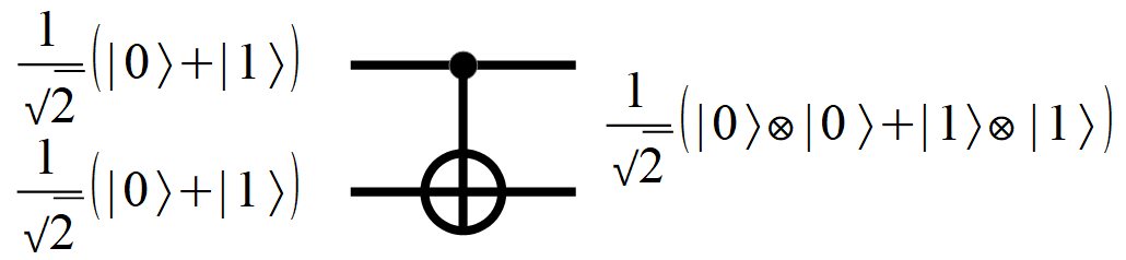
Figure 1: Cnot gate aplied to state $|\psi\rangle$

II.3 Open systems

When we have partial information of the state, i.e. we only have information of a subsystem of the total system, the state must be represented by a positive definite hermitic matrix of unitary trace, called the density matrix of a mixed state. Any pure state can be also described by a density matrix, but the inverse is not true. For the pure state $|\psi\rangle=\alpha|0\rangle+\beta|1\rangle$, the density matrix denoted by $|\psi\rangle\langle\psi|$ is

$$|\psi\rangle\langle\psi|=\left[{\begin{array}[]{cc}\alpha\alpha^{*}&\alpha\beta^{*}\\ \alpha^{*}\beta&\beta\beta^{*}\end{array}}\right].$$ (4)

The decoherence can be thought of as an unwanted interaction with the environment Alicki_2002 . When a quantum system is open, the interaction between the system $S$ and the environment $E$ can be represented as a unitary matrix of the whole system. If we only have information about the system $S$, it can no longer be described as a unitary vector, but can be described by a density matrix, which is the statistical average of an assembly of pure states.

The quantum evolution of a closed system can still be represented by a unitary matrix. When the state is represented by a density matrix $\rho$, the evolution of the state is given by $\rho^{\prime}=U\rho U^{\dagger}$ Nielsen_2000A .

II.4 Measurements

Unlike the reversible evolution of a closed process, quantum measurement is an irreversible process that collapses the quantum state. For example, for the one qubit state $|\psi\rangle$, the state collapses to $|0\rangle$ or $|1\rangle$, with probabilities ${|\alpha|}^{2}$ and ${|\beta|}^{2}$ respectively. In general, the measurements can be represented by operators. If we restrict ourselves to projective measurements, a physical observable $M$, called in this context the measurement base, can be described by the projectors $P_{i}$, generated by the eigenvectors of $M$,

$$M=\sum_{i}{\lambda_{i}P_{i}}=\sum_{i}{\lambda_{i}u_{i}^{\dagger}u_{i}}$$ (5)

where $\lambda_{i}$ and $u_{i}$ are the eigenvalues and eigenvectors respectively of $M$. Then, the probability after projective measurement of the state $\rho$ is Nielsen_2000A

$$P(i)=\textrm{Tr}\left(P_{i}\rho\right),$$ (6)

and the state after measurement becomes $\rho^{\prime}$

$$\rho^{\prime}=\sum_{i}{P_{i}\rho P_{i}^{\dagger}}.$$ (7)

III Modeling quantum errors

Every computational system is unavoidably affected by errors. In particular, the implementation of gates, the preparation of states and the measurement, can have systematic errors Greenbaum_2017 , as well as errors due to the interaction with the environment, called decoherence errors Alicki_2002 . Systematic errors could be modeled as random unitary matrices, but usually they have a preferential error direction. Both type of errors can modeled by Operator Sum Representation (Kraus_1983 ) and characterized using the isotropic index Fonseca_2017

The decoherence can be modeled by a sum of operators (Operator Sum Representation Kraus_1983 ) applied to the state of the system, determined to better adjust the noise for each type of technology.

A quantum operation over a state $\rho$ denoted $\varepsilon(\rho)$ can be expressed as a function of Kraus operators ($E_{k}$) as shown

$$\centering\varepsilon\left(\rho\right)=\sum_{k}{E_{k}}\rho E_{k}^{\dagger}\@add@centering$$ (8)

where $E_{k}$ satisfy $\sum_{k}E_{k}E_{k}^{\dagger}=I_{d}$.

III.1 Generalized Amplitude Damping error (GAD)

One of the standard models commonly used in the literature is a Generalized Amplitude Damping error (GAD), that could be interpreted as the interaction between a system and a thermal bath at fixed temperature. The model depends on two parameters: one related to the contact time with the thermal bath, represented as a probability of error $\gamma\in\left[0,1\right]$, and the second related to the temperature of the thermal bath, represented by a parameter $p\in\left(\frac{1}{2},1\right]$. For GAD error the Kraus operators are Nielsen_2000A ,

$$E_{0}=\sqrt{p}\left[{\begin{array}[]{cc}1&0\\ 0&\sqrt{1-{\gamma}}\end{array}}\right],E_{1}=\sqrt{p}\left[{\begin{array}[]{cc}0&0\\ 0&\sqrt{\gamma}\end{array}}\right],$$ (13)

$$E_{2}=\sqrt{1-p}\left[{\begin{array}[]{cc}\sqrt{1-\gamma}&0\\ 0&1\end{array}}\right],E_{3}=\sqrt{1-p}\left[{\begin{array}[]{cc}0&0\\ \sqrt{\gamma}&0\end{array}}\right]$$ (18)

III.2 Systematic errors

In addition to a decoherence error, quantum computers suffer from systematic errors like classical machines. The error can be expressed by a rotation $G$, which could have a preferential direction in space. For example, a deviation $\epsilon$ by rotation in $X$ direction, can be represented by the unitary matrix $G=e^{i\epsilon X}$ where the resulting state due to error$\rho$ is

$$\varepsilon(\rho)=G\rho G^{\dagger}$$ (19)

III.3 Isotropic index

To identify and characterize the errors, the isotropic index given in Fonseca_2017 is used. This index separates the part that cannot be corrected due to the total loss of information, called weight $w$, and the misalignment $A$ with respect to the expected reference state that, theoretically could be corrected. Considering the pure reference state of $n$ qubits, $\rho_{\phi}=|\phi\rangle\langle\phi|$, and the decomposition of a state $\rho$ after a noisy process, $\rho=p\frac{I}{2^{n}}+(1-p)\hat{\rho}$. The double index is defined as:

• The Isotropic Alignment $A$,

  $$A=Fid(\hat{\rho},\rho_{\phi})-Fid(\hat{\rho},\rho_{N\phi})$$ (20)

  where $Fid$ is the fidelity between quantum states, and $\rho_{N\phi}=\frac{I-\rho_{\phi}}{2^{n}-1}$ is the orthogonal isotropic mixed state of $\rho_{\phi}$.

• The isotropic weight $w=2^{n}\lambda$, with $\lambda$ being the smallest eigenvalue of $\rho$.

The alignment $A$ takes values in the interval $[-1,1]$. When it is completely aligned with the pure reference state $|\phi\rangle$ $A=1$ and, when it is completely misaligned, $A=-1$. The weight take values in the interval $[0,1]$. When the state $\rho$ is pure $w=0$ (the inverse is true only for one qubit state) and for a state without any information, i.e. maximum mixedness, $w=1$.

IV Error analysis on Deutsch Algorithm

IV.1 Deutsch Algorithm

The Deutsch quantum algorithm, one of the first proposed, solves in the framework of quantum computing a problem that cannot be solved in a unique step of calculation using classical computation. Although the algorithm proposed by David Deutsch is not of immediate application, it is the basis of important algorithms based on oracles such as Grover’s search of known advantage over standard computation.

The idea is defined as follows; given a black box, known as the oracle, which consists of an unknown binary function of one bit $f\left(x\right):\{0,1\}\rightarrow\{0,1\}$, the goal is to decide in a deterministic way if the function is balanced or constant using the oracle only one time. The classical algorithms need two instances of application of the oracle to solve the problem in a deterministic way, while quantum Deutsch algorithm uses the oracle a single instance, as long as there are no errors in the calculation process. The Deutsch algorithm can be summarized in the following scheme shown in the Figure 2.

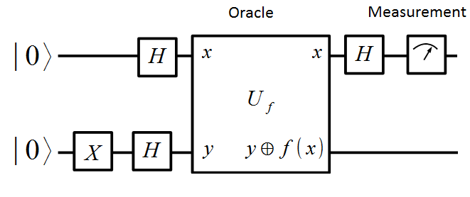
Figure 2: The Deutsch Algorithm

Beginning with the two-qubit initial state $|0\rangle\otimes|0\rangle$, a $X$ gate is applied in the second qubit getting $|0\rangle\otimes|1\rangle$. After applying a Hadamard transform to each qubit, the result is $\frac{1}{2}\left(|0\rangle+|1\rangle\right)\otimes\left(|0\rangle-|1\rangle\right)$. Applying the oracle (with one of four possible binary functions) to the current state, and ignoring the second qubit (because at this stage the qubits are independent), we get

$$\frac{1}{\sqrt{2}}\left[|0\rangle+\left(-1\right)^{f(0)\oplus f(1)}|1\rangle\right]$$ (21)

Finally, applying a Hadamard transform to this state we have

$$\frac{1}{2}\left[\left(1+\left(-1\right)^{f(0)\oplus f(1)}\right)|0\rangle+\left(1-\left(-1\right)^{f(0)\oplus f(1))}\right)|1\rangle\right]$$ (22)

Then it is concluded immediately that, the result is $0$ for constant functions, and $1$ for balanced ones.

IV.2 Deutsch Algorithm (DA) implementation on IBM Q

In order to analyze the performance of the algorithm in the IBM Q machine, the four possible functions of the oracle have to be implemented, i.e, $f_{0}$ constant zero, $f_{1}$constant one, $f_{Id}$ identity and $f_{NOT}$ inverse function. Each of these functions are implemented with the previous quantum gates Table (1), and are shown in Figures (3, 4, 5, 6).

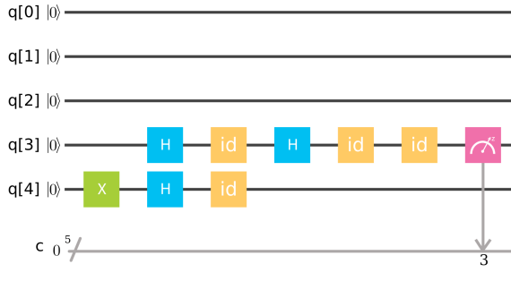
Figure 3: $DA$ IBM Q implementation, with constant zero function $f_{0}$.

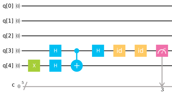
Figure 4: $DA$ IBM Q implementation, with identity function $f_{Id}$.

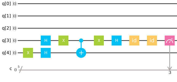
Figure 5: $DA$ IBM Q implementation, with inverse function $f_{NOT}$.

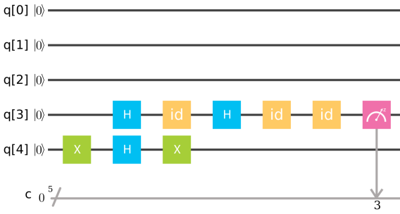
Figure 6: $DA$ IBM Q implementation, with constant one function $f_{1}$.

To study the effect of the error on the resolution of the problem, the measurement of the third qubit is made (q[3]). The result in an ideal case without error, should be 0 if the function is constant and 1 if the binary function is balanced. However, the actual result is affected due to several sources of error, which distort it with respect to the ideal case. To analyze this distortion, statistical experiments were carried out, that allow us to determine in an approximate way the representative assemble of the final state, i.e., the final mixed state denoted by $\rho$.

IV.3 Quantum state tomography (QST)

To find experimentally the density matrix of a state, a method called quantum state tomography is used Nielsen_2000A . Measurements must be made in the three bases (axes) of the space, $X,Y$ and $Z$, to recover the density matrix state. The state $\rho$ is given by Nielsen_2000A

$$\rho=\frac{1}{2}\left(I_{d}+\textrm{Tr}(\rho X)X+\textrm{Tr}(\rho Y)Y+\textrm{Tr}(\rho Z)Z\right).$$ (23)

where $\textrm{Tr}(\rho X),\textrm{Tr}(\rho Y),\textrm{Tr}(\rho Z)$, are obtained, approaching the expected value by the statistical average. For example, by spectral decomposition $Z=(+1)P_{0}+(-1)P_{1}$, then, $\textrm{Tr}(\rho Z)=\textrm{Tr}(\rho P_{0})-\textrm{Tr}(\rho P_{1})$, that by eq. (6), $\textrm{Tr}(\rho Z)=P(0)-P(1)$, where $P(0)$ and $P(1)$ are the probabilities of measuring $0$ and $1$ respectively. Similar calculations were done for $X$ and $Y$ operators.

The IBM Q computer, can measure only in the canonical base ($Z$). Then, to measure on another base, the last two identities in figures (3,4,5 and 6), must be replaced. For example, to measure in the base $X$, a rotation of a $q[3]$ qubit must be made, using in place of $I_{d}\otimes I_{d}$, the matrix $H\otimes I_{d}$, and to measure in the $Y$ basis, the identities must be replaced by $S^{\dagger}\otimes H$, where $S^{\dagger}=\left[{\begin{array}[]{cc}1&0\\ 0&-i\end{array}}\right]$, as shown in Figure 7.

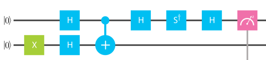
Figure 7: $DA$ IBM Q implementation, for $f_{Id}$ in $Y$ basis.

For each of the four possible binary functions, the experiments were performed $8192$ times (in IBM Q computer), and the resulting density matrices and probabilities of success are obtained and shown in Table 2.

Table 2: Probability of success for each binary function.

Binary function	Resulting matrix	Ideal result	Probability
$f_{0}$	$\left[{\begin{array}[]{cc}0.9491&0.0462-0.0664i\\ 0.0462+0.0664i&0.0509\\ \end{array}}\right]$	$0$	$0.9491$
$f_{I_{d}}$	$\left[{\begin{array}[]{cc}0.1497&0.0270-0.0160i\\ 0.0270+0.0160i&0.8503\\ \end{array}}\right]$	$1$	$0.8503$
$f_{NOT}$	$\left[{\begin{array}[]{cc}0.1748&0.1079-0.0576i\\ 0.1079+0.0576i&0.8252\\ \end{array}}\right]$	$1$	$0.8252$
$f_{1}$	$\left[{\begin{array}[]{cc}0.9495&0.0510-0.0645i\\ 0.0510+0.0645i&0.0505\\ \end{array}}\right]$	$0$	$0.9495$

IV.4 Modeling GAD error in IBM Q

After a statistical analysis of experimental data, it was determined that the model that best suited this algorithm and quantum machine (IBM Q) is a Generalized Amplitude Damping (GAD) error model [15]. Running a numerical simulation of this error and comparing with experimental data, the parameters that best adjust to the Eq. (18) for the four functions at the same time are:

$$\gamma=0.1947,p=0.7761.$$ (24)

IV.5 The Misalignment error model (MA)

The isotropic index (Fonseca_2017 ) shows that there is some misalignment for each of the 4 functions, with respect to the ideal result (see Table 3). As a result of this, we propose a method that consists of a unitary transformation applied to three qubits ( two qubits of the algorithm and one auxiliary one) that quantifies the misalignment of the state for both results, 0 and 1.

Since the result of the algorithm is a priori unknown, the model proposed applies two different unitary operators depending on the result: for $0$ it applies a $G_{0}$ gate and for $1$ it applies a $G_{1}$ gate. These conditional operations that correct the misalignment, are given by

$$G_{0}=\left[{\begin{array}[]{cc}0.996&0.053+0.069i\\ 0.090&-0.594+0.799i\\ \end{array}}\right],$$ (27)

$$G_{1}=\left[{\begin{array}[]{cc}0.994&-0.097+0.055i\\ -0.111&-0.863+0.493i\\ \end{array}}\right]$$ (30)

where the conditional operation represented in Figure 8.

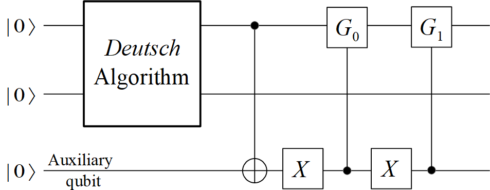
Figure 8: The Misalignment error model(MA)

The result of the model,quantified as the Fidelity between the IBM Q experimental result and the simulated one, is shown in the Table (3).

Table 3: Double Isotropic Index (Weight and Misalignment) and Fidelity between the IBM Q experimental result and the simulated error model.

Binary function	Ideal result	Weight(w)	Misalignment(A)	Fidelity
$f_{0}$	$0$	0.0873	0.9070	$0.9999$
$f_{Id}$	$1$	0.2965	0.9544	$0.9976$
$f_{NOT}$	$1$	0.3051	0.8049	$0.9996$
$f_{1}$	$0$	0.0862	0.9056	$0.9999$

V Results and Conclusions

In this work we have modeled the propagation of errors in a real quantum machine, such as IBM Q (ibmqx4). The resulting mixed states of a quantum Deutsch algorithm, are found by means of a QST method. Through the characterization using an isotropic index, the error has been modeled, in which the loss of information is given by a GAD error model, and the misaligned part by means of unitary conditional matrix (MA error model).

As shown in Table (3), the largest source of error is the decoherence, unlike the Grover algorithm, in which the misalignment is the most relevant as shown in Cohn_2016 .

The proposed error model fits very well with the experimental results, and can be the first step for the future correction of systematic errors in quantum systems.

References

- [1] Richard P. Feynman. Simulating physics with computers. Int J. Theor. Phys., 21:467–488, 1882.
- [2] David Deutsch and Roger Penrose. Quantum theory, the church;turing principle and the universal quantum computer. Proceedings of the Royal Society of London. A. Mathematical and Physical Sciences., 400(1818):97–117, 1985.
- [3] Ran Raz and Avishay Tal. Oracle separation of bqp and ph. Technical report, Weizmann Institute of Science Electronic Colloquium on Computational Complexity., 2018.
- [4] V Dunjko and HJ Briegel. Machine learning & artificial intelligence in the quantum domain: a review of recent progress. Rep Prog Phys., 81(7), 2018.
- [5] https://www.research.ibm.com/ibm-q IBM quantum experience.
- [6] Lov K. Grover. A fast quantum mechanical algorithm for database search. In Proceedings of the twenty-eighth annual ACM symposium on Theory of Computing., 1996.
- [7] Peter W. Shor. Scheme for reducing decoherence in quantum computer memory. Phys. Rev. A, 52:R2493–R2496, Oct 1995.
- [8] Simon J Devitt, William Munro, and Kae Nemoto. Quantum error correction for beginners. Reports on progress in physics. Physical Society (Great Britain)., 76:076001, 06 2013.
- [9] Matthew Otten and Stephen K. Gray. Recovering noise-free quantum observables. Phys. Rev. A., 99:012338, Jan 2019.
- [10] Daniel Gottesman. Quantum error correction and fault-tolerance. Encyclopedia of Mathematical Physics., 08 2005.
- [11] David Deutsch and Richard Jozsa. Rapid solution of problems by quantum computation. Proceedings of the Royal Society of London. Series A: Mathematical and Physical Sciences., 439(1907):553–558, 1992.
- [12] Davide Ferrari and Michele Amoretti. Efficient and effective quantum compiling for entanglement-based machine learning on ibm q devices. International Journal of Quantum Information, 16(08):1840006, 2018.
- [13] Diego Riste, Marcus P. da Silva, Colm A. Ryan, Andrew W. Cross, Antonio D. Córcoles, John A. Smolin, Jay M. Gambetta, Jerry M. Chow, and Blake R. Johnson. Demonstration of quantum advantage in machine learning. npj Quantum Information, 3, 2017.
- [14] Robin Harper and Steven T. Flammia. Fault-tolerant logical gates in the ibm quantum experience. Phys. Rev. Lett., 122:080504, Feb 2019.
- [15] André L. Fonseca de Oliveira, Efrain Buksman, Ilan Cohn, and Jesús García López de Lacalle. Characterizing error propagation in quantum circuits: the isotropic index. Quantum Information Processing, 16(2):48, 2017.
- [16] Michel A. Nielsen and Isaac L. Chuang. Quantum computation and quantum information. Cambridge University Press., 2000.
- [17] Harold V. Henderson and S. R. Searle. The vec-permutation matrix, the vec operator and kronecker products: a review. Linear and Multilinear Algebra, 9(4):271–288, 1981.
- [18] Robert Alicki, Michal Horodecki, Pawel Horodecki, and Ryszard Horodecki. Dynamical description of quantum computing: Generic nonlocality of quantum noise. Phys. Rev. A., 65:062101, May 2002.
- [19] Daniel Greenbaum and Zachary Dutton. Modeling coherent errors in quantum error correction. Quantum Science and Technology, 3(1), 2017.
- [20] K. Kraus. Lecture notes in physics. In States, Effects and Operations. Fundamental Notions of Quantum Theory., volume 190. Springer-Verlag, 1983.
- [21] Ilan Cohn, André L. Fonseca De Oliveira, Efrain Buksman, and Jesús García López De Lacalle. Grover’s search with local and total depolarizing channel errors: Complexity analysis. International Journal of Quantum Information, 14(02):1650009, 2016.