High-statistics modeling of complex pedestrian avoidance scenarios

Abstract

Quantitatively modeling the trajectories and behavior of pedestrians walking in crowds is an outstanding fundamental challenge deeply connected with the physics of flowing active matter, from a scientific point of view, and having societal applications entailing individual safety and comfort, from an application perspective.
In this contribution, we review a pedestrian dynamics modeling approach, previously proposed by the authors, aimed at reproducing some of the statistical features of pedestrian motion. Comparing with high-statistics pedestrian dynamics measurements collected in real-life conditions (from hundreds of thousands to millions of trajectories), we modeled quantitatively the statistical features of the undisturbed motion (i.e. in absence of interactions with other pedestrians) as well as the avoidance dynamics triggered by a pedestrian incoming in the opposite direction. This was accomplished through (coupled) Langevin equations with potentials including multiple preferred velocity states and preferred paths. In this chapter we review this model, discussing some of its limitations, in view of its extension toward a more complex case: the avoidance dynamics of a single pedestrian walking through a crowd that is moving in the opposite direction. We analyze some of the challenges connected to this case and present extensions to the model capable of reproducing some features of the motion.

1 Introduction

Quantitatively understanding the motion of pedestrians walking in public shared spaces is an outstanding issue of increasing societal urgency. The scientific challenges associated with the understanding and modeling of human dynamics share deep connections with the physics of active matter and with fluid dynamics bellomo2012modeling ; moussaid2009collective ; Moussadrspb.2009.0405 ; Lutz . Growing urbanization yields higher and higher loads of users on public infrastructures such as station hubs, airports or museums. This translates into more complex, high-density, crowd flow conditions, and poses increasing management challenges when it comes to ensuring individual safety and comfort. Achieving a quantitative comprehension and developing reliable models for the crowd motion may help, for instance, in the design of facilities or optimize crowd management.

Many among the proposed physical models for crowds dynamics rely on the analogy between pedestrians and active particles hughes2003flow . Either at the micro-, meso- or macro-scopic scale bellomo2012modeling , pedestrians are usually represented as self-propelling particles whose dynamics is regulated by ad-hoc social interaction potentials (cf. reviews cristiani2014multiscale ; helbing2001traffic ). While many features of crowd dynamics have been qualitatively captured by such modeling strategies (e.g., negative correlation between crowd density and average walking velocity, intermittent behavior at bottlenecks, formation of lanes in presence of opposing crowd flows seyfried2009new ; helbing1995PRE ), our quantitative understanding remains scarce, especially in comparison with other active matter systems RevModPhys.85.1143 . This likely connects with the difficulty of acquiring high-quality data with sufficient statistical resolution to resolve the high variability exhibited by pedestrian behavior. Such variability includes, for instance, different choice of paths, fluctuations in velocity, rare events, as stopping or turning around corbetta2016fluctuations . Underlying a quantitative comprehension is the capability of explaining and modeling a given pedestrian dynamics scenario, including the variability that is measurable across many statistically independent realization of the same scenario.

In this chapter we discuss the challenges connected to the quantitative modeling of a relevant and ubiquitous –yet conceptually simple– crowd dynamics scenario which involves one pedestrian, onward referred to as the target pedestrian, walking in a crowd of $N$ other pedestrians that are going in the opposite direction. We shall identify this scenario as $1$vs.$\,N$, of which, in Fig. 1, we report four consecutive snapshots taken from real-life recordings. Our analysis employs unique measurements collected through a months-long, 24/7, real-life experimental campaign that targeted a section of the main walkway of Eindhoven train station, in the Netherlands. Thanks to state-of-the-art automated pedestrian tracking technologies, fully developed in house corbetta2014TRP ; corbetta2016fluctuations ; corbetta2016continuous ; corbetta2018physics ; kroneman2018accurate , we collected millions of high-resolution pedestrian trajectories including hundreds of occurrences of $1$vs.$\,N$ scenarios.

(a)

(b)

(c)

(d)

Figure 1: Avoidance scenario, $1$vs.$\,N$, involving the target pedestrian walking towards the right (red trajectory) while a crowd of pedestrians proceeds in opposite direction (blue trajectories). We report four snapshots in chronological order. The target pedestrian escapes collisions by walking diagonally with respect to the longitudinal axis of the corridor (the most likely, in some sense “natural”, walking direction that, in this figure, corresponds to the horizontal direction). In the scenario considered, $N$ is the number of pedestrians walking in opposition to the target that have appeared in the field of view of our sensors in the time window when the target was present. Furthermore, we restrict to scenarios in which no person walking in the same direction of the target is present.

In previous works, we explored such condition in the low density limit. In particular, we proposed quantitative models for the case of a pedestrian walking undisturbed ($1$vs.$\,0$) corbetta2016fluctuations and for the case of a pedestrian avoiding a single individual coming in the opposite direction ($1$vs.$1$) corbetta2018physics . This contribution addresses the complexity, from the modeling and from the data analytic points of view, arising when dealing with the $1$vs.$\,N$ generalization. Our final model, assuming a superposition of pair-wise interactions having the form proposed in corbetta2018physics , involves the Newton-like dynamics

$$\ddot{z}_{1}=F(\dot{z}_{1})+\mathcal{N}(\,\{K(z_{1},x_{i}),i=2,\ldots,N+1\}\,)+\sigma\dot{W},$$ (1)

where $z_{1}$ is a state variable including the position of the target pedestrian, as well as their desired path and the $\{x_{i}\}$’s ($i=2,\ldots,N$) are the positions of the opposing pedestrians, $F(\dot{x_{1}})$ is an active term (modeling pedestrians self-propulsion), that regulates the onward motion of the target pedestrian, $K(x_{1},x_{i})$ is the pair-wise social interaction force between the target and the $i$-th individual, $\mathcal{N}(\cdot)$ is a (non-linear) superposition rule for the pair-wise forces. Finally, a white Gaussian noise term $\dot{W}$, with intensity $\sigma$, provides for stochastic fluctuations.

The present analysis shows, on the basis of high statistics measurements, how simplifying hypotheses based on symmetry made for the $1$vs.$\,0$ and $1$vs.$1$ cases (corbetta2016fluctuations ; corbetta2018physics ) do not hold in the general $1$vs.$\,N$ case (as could have been expected, since the influence of the boundary becomes relevant). Furthermore, we discuss how the interplay of the propulsion dynamics, determined by $F(\dot{z}_{1})$, and the presence of many interaction forces, determined by the term $\mathcal{N}(\cdot)$, may yield nonphysical effects. We present therefore some modifications to Eq. (1) that enable to recover features of the observed dynamics at the “operational level” (e.g. local collision avoidance movements, cf. hoogendoorn2002normative for a reference). This will open the discussion on how to perform data acquisition and how to achieve quantitative modeling to address the dynamics at the, so called, “tactical level”, in which broader-scale individual decisions are taken. These include, for instance, the definition of a preferred path, selected by each individual within the current room/building, to reach a desired destination.

This chapter is structured as follows: in Sect. 2 we introduce our real-life pedestrian tracking setup; in Sect. 3 we review our previous quantitative model for pedestrians walking in diluted conditions; in Sect. 4 we discuss through physical observables the more generic $1$vs.$\,N$ scenario, and introduce some of the complexities connected to its analysis and modeling; in Sect. 5 we address generalizations of our previous model to such case. A final discussion in Sect. 6 closes the chapter.

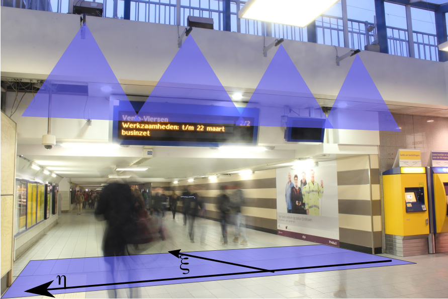
Figure 2: Picture of the pedestrian tracking setup in the main walkway of Eindhoven train station where the data described here were collected. We overlay a sketch of the measurement area, reported at the floor level, and of the initial part of the view-cones of the four depth sensors used to acquire raw depth data. As the sensors had overlapping view, we could acquire (after appropriate data fusion) continuous depth maps of the full measurement area, as those in Fig. 1 (the picture is taken facing the city center, i.e. the observer is walking a trajectory analogous to that of the target pedestrian in Fig. 1). The axes corresponding to the physical coordinates $(\xi,\eta)$ are also sketched (the canonical $(x,y)$ coordinates are here reserved for the position of a pedestrian in reference to their preferred path).

2 Measurement setup and $1$vs. N avoidance scenario

In this section, we briefly review the measurement campaign and the technique employed to collect the data that we consider throughout this chapter. Relevant references for the details of the campaign and of the measurement technique are also supplied. Then we provide a formal definition which unambiguously identifies $1$vs.$\,N$ scenarios.

The pedestrian dynamics data considered have been collected in the period Oct. 2014 – Mar. 2015 in a 24/7 pedestrian trajectory acquisition campaign in the main walkway of Eindhoven train station corbetta2016continuous (see Fig. 2). The measurements were collected through a state-of-the-art pedestrian tracking system, built in-house, and based on an array of overhead depth sensors (Microsoft Kinect™  Kinect ). The sensors view-cone were in partial overlap and allowed us to acquire data from a full transversal section of the walkway; our observation window had a size of about $9\,m$ in the transversal direction and of $3\,m$ in the longitudinal direction.

Depth sensors provide depth maps at a regular frame rate (in our case $15\,$ Hz), i.e. the distance field between a point and the camera plane. Examples of depth maps (with superimposed tracking data) are reported in Fig. 1. Notably, depth maps are non-privacy intrusive: no features allowing individual recognition are acquired. Nevertheless, depth maps enable accurate pedestrian localization algorithms (see brscic2013person ; corbetta2014TRP ; seer2014kinects for general conceptual papers about the technique, corbetta2016continuous for technical details about this campaign, and kroneman2018accurate for a more recent, highly-accurate, machine learning-based localization approach).

Our measurement location was crossed daily by several tens of thousands people and, depending on weekday and hour, the site underwent different crowd loads. Pedestrians could often walk undisturbed at night hours or, more rarely, during off-peak times (i.e. late morning and early afternoon). Else, our sensors could measure highly variable crowding conditions ranging from uni-directional to bi-directional flows with varying density levels.

We consider here scenarios that involve exactly one target pedestrian walking to either of the two possible directions while other $N$ individuals are walking towards the opposite side. This means that in accordance to our recording, the trajectory of the target pedestrian has been perturbed exclusively by these further $N$, and no other pedestrian walking in the direction of the target was observed simultaneously (and thus in the neighborhood). In corbetta2018physics we proposed a graph-based approach to describe these conditions and to efficiently find them within large databases of Lagrangian data.

3 Physics and modeling of the diluted dynamics ($1$vs.$\,0$ and $1$vs.$1$)

In this section we review the model for diluted pedestrian motion and pairwise interactions that we proposed in our previous papers corbetta2016fluctuations and corbetta2018physics . We consider a crowd scenario to be diluted whenever the target pedestrian can move freely from the influence of other peer pedestrians (e.g. incoming, or moving close by, i.e. $1$vs.$\,0$ condition) or they are just minimally affected ($1$vs.$1$).

In diluted conditions, individuals crossing a corridor typically move following (and fluctuating around) preferred paths that develop as approximately straight trajectories. Preferred paths belong to the tactical level of movement planning, in other words, changes in preferred paths are connected to individual choices performed at level overarching fine-scale navigation movements (operational level). Without loss of generality, we consider a coordinate system such that the state of a pedestrian can be described through three position-like variables, $z=(x,y,y_{p})$, and relative velocities (in the following indicated, respectively, with $u$, $v$, and $\dot{y}_{p}$). In particular, $y_{p}$ parameterizes the preferred path (that we assume parallel to the $x$-axis) and $(x,y)$ identifies the instantaneous pedestrian position.

In this reference system, as $x$ varies, individuals approach (or, conversely, get farther apart from) their destinations. In the transversal direction, fluctuations of amplitude $\tilde{y}=y-y_{p}$ occur around the center of the preferred path, $y_{p}$. In absence of avoidance interactions with other pedestrians, we expect $\dot{y}_{p}=0$, at least on the tactical time-scale. Conversely, we expect that the need of avoiding a pedestrian incoming with opposite velocity will be reflected in a dynamics for $y_{p}$.

Following corbetta2018physics , we model the motion of a target pedestrian in a $1$vs.$1$ condition with a Langevin dynamics as

$$\frac{\mathrm{d}x}{\mathrm{d}t} =u(t)$$ (2)

$$\frac{\mathrm{d}y}{\mathrm{d}t} =v(t)$$ (3)

$$\frac{\mathrm{d}u}{\mathrm{d}t} =-4\alpha_{i}u(u^{2}-u_{p,i}^{2})+\sigma\dot{W}_{x}-e_{x}F_{short}$$ (4)

$$\frac{\mathrm{d}v}{\mathrm{d}t} =-2\lambda v-2\beta(y-y_{p})+\sigma\dot{W}_{y}-e_{y}F_{short}+F_{vision},$$ (5)

$$\frac{\mathrm{d}y_{p}}{\mathrm{d}t} =\dot{y_{p}}(t)$$ (6)

$$\frac{\mathrm{d}\dot{y}_{p}}{\mathrm{d}t} =F_{vision}-2\mu\dot{y}_{p}.$$ (7)

In the reminder of this section we detail the expressions and the modeling ideas underlying the preferred velocities, $u_{p,i}$, the friction terms, $-2\lambda v$ and $-\mu\dot{y}_{p}$, and the social forces $F_{short}$ and $F_{vision}$. We anticipate that $F_{short}$ and $F_{vision}$ are exponentially decaying social interaction forces depending on the distance between the target pedestrian and the other individual. Consistently, they vanish in the case of a pedestrian walking undisturbed thus, in such case, $\dot{y}_{p}=0$ holds, and the model restricts to that considered in corbetta2016fluctuations . For the sake of brevity, in Eqs. (2)-(7) we omitted the subscript “1” for the target pedestrian variables as in the notation in Eq. (1), as in the current case there is no ambiguity (i.e. $x$ should be written as $x_{1}$, and similarly for the other variables. However, the position variables of the second pedestrian, like $x_{2}$, are in fact hidden in the social force terms).

Table 1: Parameters for the model in Eqs. (2)-(7).

$1$vs.$\,0$ and $1$vs.$1$		$1$vs.$1$ only
Desired walking speed		Vision f. inter. scale
$u_{p,w}$ (walkers)	$1.29\,$ms-1	$R$	$2.4\,$m
Desired running speed		Contact-av f. inter. scale
$u_{p,r}$ (runners)	$2.70\,$ms-1	$r$	$0.6\,$m
Coeff. $U(u)$, walkers		Desired path friction
$\alpha_{w}$	$0.037\,$m-2s	$\mu$	$1.0\,$s-1
Coeff. $U(u)$, runners		Vision f. intensity
$\alpha_{r}$ (runners)	$0.0015\,$m-2s	$A$	$1.5\,$ms-2
Noise intensity		Contact-av f. intensity
$\sigma$	$0.25\,$ ms-3/2	$B$	$0.7\,$ms-2
Transv. confinement		Vision f. angular dep.
$\beta$	$1.765\,$ m-2s	$\chi_{vision}$ (threshold)	$20\,^{\circ}$
Transv. friction		Contact-av f. angular dep.
$\lambda$	$0.297\,$s-1	$\chi_{short}$ (threshold)	$90\,^{\circ}$
runner $\%$ in $1$vs.$\,0$	$4.02$%	runner $\%$ in $1$vs.$1$	$0.2\,$%

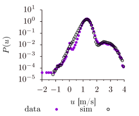
(a)

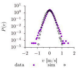
(b)

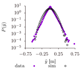
(c)

Figure 3: Probability distribution functions of walking velocity and positions for pedestrians walking undisturbed $1$vs.$\,0$: comparison between measurements (purple dots) and simulations of Eq. (2)-(7) in absence of interaction forces (circle markers, simulation parameters in Tab. 1). The panels contain respectively (a) longitudinal velocities ($u$), (b) transversal velocities ($v$), (c) transversal positions with respect to the preferred path ($\tilde{y}=y-y_{p}$). Pedestrians walk most frequently at around $1.29\,$m/s (cf. (a)). Besides, we observe a small fraction of running pedestrians, about $4\,\%$, contributing to the hump at above $2\,$m/s and pedestrians turning back, providing negative velocities contributions. (b) Transversal fluctuations in velocity appear to be well-approximated by a Gaussian distribution, while (c) transversal positions exhibit small deviations from a Gaussian behavior. The model captures quantitatively the complete longitudinal velocity statistics including the running hump as well as the inversion events. The transversal dynamics is also well approximated as a stochastic damped harmonic oscillator (Eq. (3) and (5)).

The second order dynamics in Eqs. (2)-(7) includes the interplay of activity, fluctuations and interactions. In corbetta2016fluctuations we showed that, in absence of interactions, the motion of a pedestrian is characterized by small and frequent Gaussian velocity fluctuations around a preferred and stable velocity state, $(u,v)=(\pm u_{p},0)$. Large fluctuations can be observed as well, although rarely: for a narrow corridor, the prominent case is the transition between the two stable velocity states $u\rightarrow-u$, which comes with a direction inversion. The simplest conceivable velocity potential, $U=U(u)$, allowing for this phenomenology is a symmetric polynomial double well with minima at $u=\pm u_{p}$, i.e. $U(u)\sim(u^{2}-u_{p}^{2})^{2}$, from which the force term $-\partial_{u}U(u)\sim-u(u^{2}-u_{p}^{2})$ in Eq. (4). In combination with a small Gaussian noise (term $\sigma\dot{W}_{x}$), this yields small-scale Gaussian fluctuations and rare Poisson-distributed inversion events (see also corbetta2018path for a path-integral based derivation of the event statistics), both in extremely good agreement with the data (cf. corbetta2016fluctuations ). In Eq. (4), we included the subscript $i$ on the preferred velocity and on the force intensity coefficient, respectively $u_{p,i}$ and $\alpha_{i}$, to allow independent “populations” of pedestrians having different moving features (e.g. walking vs. running) combined in different percentages (see Table 1). In Fig. 3(a) we report a comparison of the probability distribution function of the longitudinal velocity $u$ for undisturbed pedestrians in case of measurements and simulated data, which shows a remarkable agreement.

We treat the transversal dynamics as a damped stochastic harmonic oscillator centered at $y_{p}$, respectively via the friction force $-2v\lambda$, the Gaussian noise $\sigma\dot{W}_{y}$ and the harmonic confinement $-2\beta(y-y_{p})$. This yields Gaussian fluctuations of $v$ and $\tilde{y}$, which are also in very good agreement with the measurements, Figs. 3(b-c). For both the longitudinal and transversal components we employ white in time (i.e. $\delta$-correlated) and mutually uncorrelated Gaussian noise forcing ($\dot{W}_{x}$, $\dot{W}_{y}$), with equal intensity ($\sigma$), as validated in corbetta2016fluctuations . Our hypotheses on the noise structure are guided by simplicity, yet they are somehow arbitrary and not mandatory Lutz .

Interactions enrich the system of social force-based coupling terms and of a second order deterministic dynamics for $y_{p}$ (Eqs. (6)-(7)). We consider two conceptually different coupling forces:

• a long-range, vision-based, avoidance force

  $$F_{vision}(x_{1},y_{1},x_{2},y_{2})=-\mathrm{sign}(e_{y})A\,\mathrm{exp}(-d^{2}/R^{2})\chi_{vision}(\tilde{\theta}),$$ (8)

  where $e_{y}$ is the $y$ component of the unit vector pointing from $(x_{1},y_{1})$ to $(x_{2},y_{2})$ (i.e. the unit vector $(e_{x},e_{y})=(x_{2}-x_{1},y_{2}-y_{1})/d$, $d$ being the Euclidean distance between the positions of the pedestrians, $d=||(x_{2}-x_{1},y_{2}-y_{1})||_{2}$), $\tilde{\theta}$ is the angle between the $x$-axis and the distance vector $(x_{2}-x_{1},y_{2}-y_{1})$, $\chi_{vision}(\tilde{\theta})$ is the indicator function that is equal to $1$ if $|\tilde{\theta}|\leq 20\,^{\circ}$ and vanishing otherwise, $A$ and $R$ are an amplitude and a scale parameter.

• a short-range contact-avoidance force

  $$F_{short}(x_{1},y_{1},x_{2},y_{2})=B\,\mathrm{exp}(-d^{2}/r^{2})\chi_{short}(\tilde{\theta}),$$ (9)

  where $\chi_{short}(\tilde{\theta})$ is an indicator function that is equal to $1$ if $|\tilde{\theta}|\leq 90\,^{\circ}$ and vanishing otherwise, $B$ and $r$ are an amplitude and a scale parameter.

Note that $F_{vision}$ operates on the transversal direction only and appears both in Eq. (5) and Eq. (7). In other words, it influences the dynamics of $\tilde{y}$ only through $\dot{y}_{p}$. In fact, combining Eqs. (5) and (7), the evolution of $\tilde{y}$ satisfies

$$\frac{d^{2}\tilde{y}}{dt^{2}}=-2\lambda\frac{d\tilde{y}}{dt}-2(\mu-\lambda)\dot{y}_{p}-2\beta\tilde{y}+\sigma\dot{W}_{y}-e_{y}F_{short}.$$ (10)

Vision and contact avoidance forces allow to reproduce the overall avoidance dynamics. We analyze this by considering how the pedestrian distance, projected on the $y$ direction, transversal to the motion, changes during the avoidance maneuvers. In particular, we consider three projected distances:

1. $\Delta y_{i}$: the absolute value of the transversal distance, as the pedestrians appear in our observation window;

2. $\Delta y_{s}$: the absolute value of the transversal distance, at the instant of minimum total distance between the pedestrians;

3. $\Delta y_{e}$: the absolute value of the transversal distance when the pedestrians leave our observation window.

In Fig. 4, we report the conditioned averages of these distance, comparing measurements and simulations. In particular, Fig. 4(a) contains the average transversal distance when the two pedestrians are closest (i.e. side-by-side, $e(\Delta y_{s})$), conditioned to their entrance distance ($\Delta y_{i}$). We observe that for $\Delta y_{i}\lessapprox 1.4\,$m avoidance maneuvers start and pedestrians move laterally to prevent collisions. In case of pedestrians entering facing each other ($\Delta y_{i}\approx 0$), on average they establish a mutual transversal distance of about $75\,$cm. As experience suggests, for large transversal distances no concrete influence is measured. In Fig. 4(b), we report the average transversal distance as the two pedestrians leave the observation area ($e(\Delta y_{e})$) conditioned to the transversal distance at the moment of minimum distance ($\Delta y_{s}$). We observe that, on average, the mutual distance remains unchanged. This means that the act of avoidance impacts on the preferred path, which drifts laterally as collision is avoided and then is not restored. We can read this as an operational-level dynamics (avoidance gesture), that impacts on the coarser-scale tactical-level dynamics, as the preferred path gets changed. Remarkably, the model is capable to quantitatively recover these features. We refer the interested reader to corbetta2018physics where we additionally discuss the full conditioned probability distributions of the transversal distances plus other statistical observables such as pre- and post-encounter speed and collision counts.

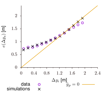
(a)

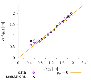
(b)

Figure 4: Average conditioned transversal distance between two pedestrians in a $1$vs.$1$ condition: comparison between data and simulations. (a) Average, $e(|\Delta y_{s}|)$, of absolute lateral distance when at the closest point (side-by-side, $y$-axis) conditioned to the absolute lateral distance when at the entrance ($\Delta y_{i}$, $x$-axis). (b) Average, $e(|\Delta y_{e}|)$, of absolute lateral distance when at the exit ($y$-axis), conditioned to the absolute lateral distance when side-by-side ($|\Delta y_{s}|$, x-axis). The diagonal line identifies cases in which the transversal distance between the pedestrians has not changed from one measurement point to the next, which can be interpreted as a preferred path that remained unchanged as pedestrian crossed the observation window. The model in Eqs. (2)-(7) reproduce with high accuracy the avoidance dynamics.

Note that both scenarios considered so far, $1$vs.$\,0$ and $1$vs.$1$, feature a translational symmetry in the transversal direction, i.e. the dynamics is unchanged by rigid translations: $y\rightarrow y+c$, $y_{p}\rightarrow y_{p}+c$.

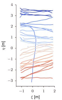
(a)

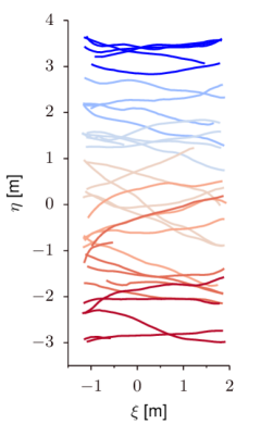
(b)

Figure 5: Random selection of trajectories of pedestrians walking from the bus station side of the train station toward the city center (from left to right in this reference), in case (a) of pedestrians walking alone (i.e. $1$vs.$\,0$) or (b) in case $1$vs.${\,10}$. In case of pedestrians walking alone (a), the trajectories are mostly rectilinear, superimposing small fluctuations to an intended path. In rare cases we observe large deviations, as, for instance, inversions or drastic trajectory changes. In case of target pedestrians facing a crowd (b), the trajectories exhibit ample deviations following the need of avoiding incoming individuals. Avoidance maneuvers effectively increase fluctuations, direction changes along the path, and dispersion in the position in which the pedestrian leaves the observation zone. The trajectories are here reported in physical coordinates $(\xi,\eta)$ (cf. Fig. 2).

4 Observables of the $1$vs. N scenario

As a target pedestrian walks avoiding an increasing number of other individuals moving in the opposite direction (i.e. $1$vs.$\,N$, $N>1$), his or her trajectory acquires a richer and more fluctuating dynamics. In Fig. 5, we compare trajectories of pedestrians moving towards the city center (i.e. from left to right) in case of undisturbed pedestrians ($1$vs.$\,0$, Fig. 5(a)) and in case $1$vs.${\,10^{+}}$ (i.e. $N\geq 10$, Fig. 5(b)). Note that the trajectories are reported in the physical coordinate system, $(\xi,\eta)$, where the first component is parallel to the span of the corridor and the second component is in the transversal direction. These coordinates must not be confused with $(x,y,y_{p})$ which are instead aligned with the individual preferred paths. In this random sample of trajectories, it is already visible that in the case of individual pedestrians the absence of incoming “perturbations” allow less pronounced fluctuations that, in most of the cases occur around well-defined straight paths, i.e., by definition, the preferred paths. It must be noticed that these preferred path are not, generally, parallel to the $\xi$-axis. Rare largely deviating trajectories also appear, in the figure it is reported a case of trajectory inversion. Conversely, the presence of incoming pedestrians, in addition to enhancing small-scale fluctuations, frequently yields curved or S-like trajectories for the target individual, as an effect of successive avoidance maneuvers.

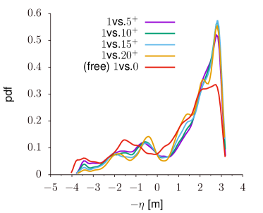
(a)

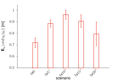
(b)

Figure 6: (a) Probability distribution function of traversal positions, $\eta$, for target pedestrians in free flow ($1$vs.$\,0$) vs. an increasing number of incoming pedestrians (note that the $\eta$ axis is flipped to $-\eta$ with respect to the reference in Fig. 2 such that the right side of the plot coincides with the right side of the corridor for an observer located as in Fig. 2). Although the corridor is rectangular, the position distribution is not uniform. We believe that this possibly connects both to cultural biases and to the geometry upstream with respect to the observed areas. The entrance area is, in fact, asymmetric and wider on its right end. As the incoming pedestrians increase in number, so does the tendency to choose for the right side of the corridor. (b) Aggregated statistics of the outlet position dispersion conditioned to inlet location and incoming flow. The inlet distribution in (a) maps to an articulated outlet distribution with dependency on inlet and flow conditions. We report it in aggregated form by averaging the conditioned standard deviation of the outlet position, $std(\eta_{e}|\eta_{i})$, over the inlet position $\eta_{i}$, (hence, no further dependency $\eta_{i}$ remains. The evaluation is restricted to the bulk of the flow, $-1.5\,\text{m}\leq\eta_{i}\leq 3.1\,$m, i.e. measurements within half a meter from the left wall and from the right-side peak are neglected. Error bars report the standard error on the average). As the incoming crowd grows, and up to the case of $10$ incoming pedestrians, so it grows the variance in the outlet position distribution. In other words, the need of avoidance induces larger and larger deviations from the average trajectory. Further increments of the number of incoming pedestrians yield a reduction in dispersion. This likely connects with the fact that the target pedestrian remains “funneled” by the incoming crowd. According to (a) this happens with highest probability in proximity of the right-hand side wall.

An incoming crowd enhances the tendency of the target pedestrian to keep the right-hand side. In Fig. 6(a) we report the probability distribution function of transversal positions (in the corridor reference, i.e. $pdf(\eta)$). As the number of incoming pedestrians increases, the $\eta$ distribution increasingly peaks on the right-hand side, remaining focused in the close proximity of the wall. Out of the bulk and close to a wall, avoidance remains easiest and straight trajectories can be followed, see Fig. 5(b).

On the opposite, avoidance maneuvers are strongest in the bulk, and of magnitude increasing with the number, $N$, of incoming pedestrians, at least up to a threshold. In Fig. 6(b) we report the aggregated measurement of the dispersion in the transversal position as the target pedestrian leaves our observation window, $\eta_{e}$, conditioned to their entrance position, $\eta_{i}$. Specifically we report the average, computed over $\eta_{i}$, of the standard deviation of $\eta_{e}$ conditioned to $\eta_{i}$, in formulas $\textbf{E}_{\eta_{i}}(\,std(\eta_{e}|\eta_{i})\,)$. In other words, for each entrance location (considered after a binning of the area, $-1.5\,\text{m}\leq\eta_{i}\leq 3.1\,$m, into $20$ uniformly spaced sub-regions), we consider the conditioned standard deviation of exit location(s). As this aims at measuring the “point-dispersion” from each individual entrance site, we average all these point-dispersion measurements. We notice that the average point-dispersion increases by $20\%$ from scenario $1$vs.$\,0$ to $1$vs.${\,5^{+}}$ and by a further $10\%$ when restricting to $1$vs.${\,10^{+}}$. If we restrict to a larger number of incoming pedestrians, the average dispersion starts reducing. This is likely a consequence of the fact that, in many cases, the target pedestrian remains “funneled” in a narrow space left by the incoming crowd.

Considering the increment in the variability and in the fluctuations of the trajectories for the generic $1$vs.$\,N$ case, for large $N$, and the relative shortness of our observation window (about $3\,$m), contrarily to the $1$vs.$\,0$ and $1$vs.$1$ cases, our data only allows us to evaluate operational-level movements. In other words, within our observation window we can collect statistics about the fine scale avoidance but not on the way the preferred path gets modified on a longer time scale. On this bases, in the next section we present a model for the $1$vs.$\,N$scenario.

Figure 7: The longitudinal walking dynamics of a pedestrian in diluted conditions, according to Eqs. (2)-(4), is defined by the interplay of a velocity gradient force, $-\partial U$, that brings the system toward a stable state (in this case, say $u=+u_{p}$. A sketch of the potential $U$ is reported in blue), a random forcing, $\sigma W_{x}$, that brings the system away from the stable state (and possibly yields transitions between the stable states), and the longitudinal component of the short-range, contact avoidance, force, $F_{short}$. As these forces linearly accumulate when $N$ increases, the system gets more and more “unbalanced” toward the unstable state $u=0$ or the negative velocities. In other words excessive forcing increases the hopping probability towards negative velocities and effectively reduces the potential barrier that separates the stable states. Although it is reasonable to expect that the probability of trajectory inversion increases in presence of a large incoming crowd, the phenomenon has to be probabilistically characterized. Here we bring this probability (unrealistically high for the original double-well potential, as in corbetta2016fluctuations ; corbetta2018physics ) to zero, by considering a Taylor approximation of the potential around the positive velocity stable state, i.e. $U(u)\approx C(u-u_{p})^{p}$, where $C$ is a positive constant. Finally, in presence of a large incoming crowd, the desired walking velocity (that one would keep in diluted flow) most likely cannot be employed due to “resistance” of the surrounding crowd. Hence, the effective walking velocity is reduced (cf. fundamental diagram in corbetta2016continuous ). In presence of enough data the statistics of such reduction can be quantified. Here, focusing on the path fluctuations, we set the locally preferred velocity to the average longitudinal walking velocity of the target pedestrian. This translates the velocity potential towards velocities lower in absolute value (gray dashed line).

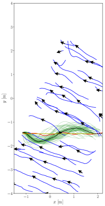
(a)

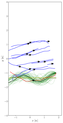
(b)

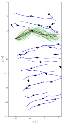
(c)

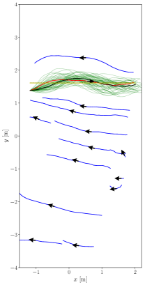
(d)

Figure 8: Comparison of measurements and simulations performed via Eqs. (11)-(16) and non-linear force superposition model (C4) in four $1$vs.$\,N$ scenarios. We consider the coordinates, $(x,y)$, aligned with the preferred path of the target pedestrian (i.e. the whole domain has been rotated accordingly). The measured trajectory of the target pedestrian is reported in red, in blue are the measured trajectories of the incoming crowd. We display in green different target pedestrian trajectory realizations as generated by our model, and in black the classical path or the (time-)averaged simulated trajectory (cf. Eq. (17)).

5 Modeling $1$vs. N dynamics via superposition of interactions

In this section we address the generalization of the model in Eqs. (2)-(7) (cf. Sect. 3) as the number of incoming pedestrians increases. Our underlying hypothesis is the existence of a superposition rule for the pairwise vision-based and contact-avoidance forces in presence of more than one opposing pedestrian. In the next equations, we indicate these as $\mathcal{N}_{short}(\{\cdot\})$ and $\mathcal{N}_{vision}(\{\cdot\})$. To emphasize the generality of the superposition, we set the argument of these functions to the whole set of pairwise forces, in general referred to as $\{f_{i}\}$. The linear superposition rule (or linear superposition of effects, i.e. $\mathcal{N}(\{f_{i}\})=\sum_{i}f_{i}$), ubiquitous in classical physics, has been widely considered in pedestrian dynamics (e.g., cristiani2014BOOK ; helbing1995PRE ), but also it has been criticized (e.g. moussaid2011simple ). Notably, in a context of linear superposition of forces, the total force intensity may diverge in presence of a large crowd. Most importantly, however, it is likely that the individual reactions are dependent on a (weighted) selection of surrounding stimuli rather than on their blunt linear combination moussaid2011simple . In formulas, we consider the following dynamics

$$\frac{dx_{1}}{dt}=u_{1}$$ (11)

$$\frac{du_{1}}{dt}=F(u_{1})-\mathcal{N}_{short}(\{e_{x,i}F_{short,i}\})+\sigma_{x}\dot{W}_{x}$$ (12)

$$\frac{dy_{1}}{dt}=v_{1}$$ (13)

$$\frac{dv_{1}}{dt}=-2\lambda v_{1}-2\beta(y_{1}-y_{p})-\mathcal{N}_{short}(\{e_{y,i}F_{short,i}\})+\mathcal{N}_{vision}(\{F_{vision,i}\})+\sigma_{y}\dot{W}_{y}$$ (14)

$$\frac{dy_{p,1}}{dt}=\dot{y}_{p,1}$$ (15)

$$\frac{d\dot{y}_{p,1}}{dt}=-2\mu\dot{y}_{p,1}+\mathcal{N}_{vision}(\{F_{vision,i}\}),$$ (16)

here the subscripts “$1$” and $i$ ($i=2,\ldots,N+1$) identify explicitly the target pedestrian and the rest of the incoming crowd. For the sake of brevity, we used the notation $\{F_{vision,i}\}$ to indicate the set of pair-wise forces $\{F_{vision,i},i=2,\ldots,N+1\}$ between the target pedestrian and the $N$ other individuals.

The highly complex dynamics, in combination with the relative shortness of our observation window, allows us to highlight some modeling challenges connected to finding and validating functional forms to the terms in Eqs. (11)-(16). We list these here and address them through additional hypotheses or simplifications on the dynamics model.

• Bi-stable dynamics vs. contact avoidance forces. Avoidance forces inter-play with our bi-stable velocity dynamics (cf. Fig. 7). Effectively they increase the probability of hopping between the two stable velocity states and provide nonphysical trajectory inversions. Although it is reasonable to expect an higher trajectory inversion rates when a pedestrian faces a large crowd walking in opposite direction, such rate has to be probabilistically characterized. In modeling terms, we expect the height of the potential barrier $U(u_{p})-U(0)$ between the stable velocity state, $u=\pm u_{p}$, and the zero walking velocity, $u=0$, to be altered by the incoming crowd. In absence of validation data, here we simplify our model by considering a second-order Taylor expansion of the potential $U$ around $u=+u_{p}$. In this way, $u=+u_{p}$ remains the only stable state of the dynamics and trajectory inversions are therefore impossible. While this is a strong simplification, it serves the present purpose of studying $1$vs.$\,N$ scenarios.

• Preferred path. In presence of many consecutive avoidance maneuvers, as in a typical $1$vs.$\,N$ case, the trajectory of the target pedestrian is continuously adjusted. These adjustments likely include modifications of the preferred path. Our monitoring area along the longitudinal walking direction is relatively short (about $3\,$m). As such, local avoidance maneuvers (operational level) remain mostly indistinguishable for re-adjustments of the preferred path (tactical level). Therefore, we opt to address path variations as avoidance maneuvers (i.e. operational level movements). As we hypothesize that tactical-level movements are negligible, we opt to set the preferred path to the average longitudinal path measured. Longer recording sites would open the possibility of addressing statistically the dynamics of preferred paths in presence of many successive interactions.

• Preferred velocity. The diluted motion comes with a measurable notion of preferred walking velocity (or velocities in case of multiple walking modes). In Fig. 3(a) we report the pdf of the longitudinal component of the velocity for undisturbed pedestrians, $u$, displaying the superposition of two dominant behaviors, pedestrians walking and running with averages velocity $u_{p,w}=1.29m/s$, $u_{p,r}=2.70m/s$, respectively. In the generic $1$vs.$\,N$ case, we expect an “adjusted” preferred velocity depending on the surrounding traffic. In other words, although a pedestrian would keep their desired velocity constant at all times, the constraints given by the presence of other pedestrians require its temporary reduction. The velocity reduction is generally reported in average terms through fundamental diagrams (i.e. density-velocity relations seyfried2005fundamental ) that for our setup we quantified in corbetta2016continuous . At the microscopic level, we expect a number of elements influencing the adjusted preferred speed, e.g.: surrounding crowd density, geometry of and position in the domain, presence of a visible walkable free space within the incoming crowd, etc. These aspects are also likely statistically quantifiable in presence of a large enough observation window, that enables to disentangle tactical- and operational-level aspects of the dynamics. Similarly to the preferred path, here we set the preferred velocity to the average walking velocity of the target pedestrian.

• Superposition rule for vision-based interactions. Vision-based interactions are long-range, and relatively narrow angled (cf. Sect. 3 and corbetta2018physics ). This makes them mostly irrelevant in a $1$vs.$\,N$ condition as in Fig. 1, where there is limited frontal interaction as compared to interactions with other neighboring neighbors. As such, we opt to simplify the superposition rule for this forces to a linear summation, that is $\mathcal{N}_{vision}(\{f_{i}\})=\sum_{i=2}^{N+1}f_{i}$.

Given these simplifications, we consider four superposition rules for the short range contact-avoidance forces:

1. $\mathcal{N}_{short}(\{f_{i}\})=\sum_{i=2}^{N+1}f_{i}$ - this is a linear extension to Eqs. (4)-(5) and serves as a baseline reference;

2. $\mathcal{N}_{short}(\{f_{i}\})=\frac{1}{10}\sum_{i=2}^{N+1}f_{i}$ - this case is analogous (C1), but a scaling of the interaction by a factor $10$;

3. $\mathcal{N}_{short}(\{f_{i}\})=\frac{1}{10}\sum_{i=2}^{N+1}f_{i}$ and $\alpha\rightarrow 10\alpha$ - this case extends (C2) by steepening the velocity potential around the stable velocity state by a factor $10$;

4. $\mathcal{N}_{short}(\{f_{i}\})=\frac{1}{2}\max_{i}(f_{i})$ - this is a non-linear superposition of forces: because of the decreasing monotonicity of the short-range interactions, this is equivalent to consider interactions exclusively with the nearest-neighbor.

Considering the stochastic dynamics, we compare the simulations and data as follows. We sample $200$ random occurrences in a $1$vs.$\,N$ scenario from our measurement in which the target pedestrian enters in the bulk section of the domain; each scenario is similar to what depicted in Fig. 1. We specifically consider $N=10^{+}$, that according to Fig. 6(b), span among the most challenging cases in terms of variability of the paths. For each occurrence, we opt to simulate through Eqs. (11)-(16) exclusively the target pedestrian dynamics, while we update the position of the other $N$ individuals according to the data (our simulation step, $\Delta t$, is equal to the sampling period of the sensor, i.e. $(15\,\mbox{Hz})^{-1}=66\,\mbox{ms}$). Employing the measured initial position of the target pedestrian and initial velocity sampled from the target measured walking velocities, we simulate his or her dynamics, from the entrance in our observation window to the exit, for $M=50$ independent realizations. We report in Fig. 8 examples of such simulations (green lines) overlaying real measured trajectories of the target pedestrian and of the rest of the crowd (respectively in red and blue). Employing the simulated trajectories, we can compute an ensemble-averaged path, $\bar{z}^{r}_{1}(t)=(\bar{x}_{1}^{s}(t),\bar{y}^{s}_{1}(t),\bar{y}^{s}_{p,1}(t))$ (i.e., with some abuse of terminology from the quantum path integral language corbetta2018path , this would correspond to the “classical path”) as

$$\bar{z}^{s}_{1}(t)=\frac{1}{M}\sum_{k=1}^{M}z^{s}_{1,j}(t),$$ (17)

where $j$ indexes the realizations, the average is performed on the position vectors $z_{1,j}^{s}(t)=(x_{1,j}^{s}(t),y^{s}_{1,j}(t),y^{s}_{p,1,j}(t))$ and the superscript $s$ indicates that the quantities involved are from simulated data. Hence, we can compute the pdf of the instantaneous fluctuation, $d_{B}(\bar{z}^{s}_{1},z_{1})(t)$, with respect to the classical path

$$d_{B}(\bar{z}^{s}_{1},z_{1})(t)=||(\bar{x}^{s}_{1}(t),\bar{y}^{s}_{1}(t))-(x_{1}(t),y_{1}(t))||_{2},$$ (18)

where the position $z_{1}$ can be either from the simulated data themselves or from the measurements. The underlying idea is to probe how likely it is that a measured trajectory is prompted by the model, for which, a necessary condition is a similar $d_{B}$ probability distribution. Note that in the case of simulated trajectories, the distribution of $d_{B}$ gives a measure for the size of the trajectory bundle (cf. bundle of green simulated trajectories in Fig. 8).

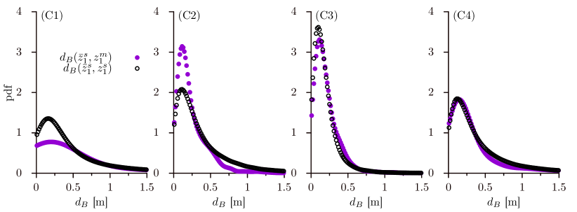
Figure 9: Probability distribution functions of the distance $d_{B}$ between the simulated classical path (i.e. the average simulated trajectory, cf. Eq. (18)) and the measured or the simulated trajectories, respectively $d_{B}(\bar{z}^{s}_{1},z^{m}_{1})$ and $d_{B}(\bar{z}^{s}_{1},z^{s}_{1})$, for short-range force superposition rules (C1)-(C4). The non-linear force superposition, considering interactions with the first-neighbor only, allows highest similarities in the distance distributions, with minimum variation of parameters with respect to the $1$vs.$1$ case.

In Fig. 9, we report the probability distribution of the distance $d_{B}$ for the four force superposition rules (C1)-(C4). We observe that a first-neighbor-only reaction (C4) yields a distance distribution, in case of measured and simulated trajectories, that is mutually closest while incorporating the least parameter variations with respect to the validated $1$vs.$1$ case. In this case, we exclusively halved the intensity of the short-range interaction force. Such reduction might be further justified by the fact that only the target pedestrian has been simulated, which included no reaction of the other pedestrians that where passively moved according to the measurements. We stress that, possibly many other superposition rules may exist: in case (C3) in fact, we achieved a good agreement between the distance distribution. Nevertheless, this involved not only a reduction of the interaction forces by a factor $10$, which may agree with a mean-field like interaction scaling (here $N\approx 10$ holds), but we needed to heavily steepen the velocity potential around the stable state, with respect to the validated value in the $1$vs.$\,0$ case, i.e. we increased $\alpha$ and so the likelihood of a pedestrian to keep their desired velocity.

6 Discussion

In this chapter we addressed complex avoidance scenarios involving one pedestrian walking in a corridor while avoiding a crowd of $N$ other individuals walking in the opposite direction, that we conveniently named $1$vs.$\,N$. Our analysis has been based on real-life data collected in an unprecedented experimental campaign held over about a one year time-span, held in the train station of Eindhoven, The Netherlands, in which millions of individual trajectories have been recorded with high space- and time-resolution. We considered this scenario a first step to tackle avoidance in non-diluted conditions; we based our analysis and modeling on our previous works on diluted $1$vs.$\,0$ and $1$vs.$1$ conditions that we briefly reviewed in the first part of the chapter.

Our contribution here is two-fold. First we evidenced, on the basis of the experimental data, complex aspects of the dynamics arising in comparison to a diluted flow: namely the increased randomness in the motion, both in terms of small scale fluctuations and of avoidance maneuvers (operational level dynamics), and the increased relevance of geometric aspects. These elements also show how our current trajectory database enables to explore just a small portion of the overall $1$vs.$\,N$ dynamics, that we could mainly address in its operational aspects, while we had to make assumptions on the tactical part.

On this basis, we considered a generalization of our previous model for the diluted dynamics. Assuming the preferred path and speed known, we could show that a non-linear superposition of short-ranged contact avoidance forces, focusing on the first neighbor only, could produce a position-wise fluctuation distribution with respect to the classical path that was in better agreement with the measurements; i.e. with higher chance, the trajectories measured in real-life could have been generated by our stochastic model. It is important to stress that this is possibly one among many fitting forces superposition schemes. In fact, we could produce fluctuations distributions with good agreement between simulations and data also with a linear superposition of forces; this however required multiple parameters changes with respect to the validated baseline $1$vs.$\,0$ and $1$vs.$1$ models.

While extending the model to the $1$vs.$\,N$ case we could also point out a limitation in our $1$vs.$\,0$ modeling approach. We cast both types of identified longitudinal velocity fluctuations, i.e. the frequent and small oscillations and the rare and large path deviations (trajectory inversions), in a unified perspective through a double well potential in velocity. In presence of interaction forces among pedestrians, these interplay with the gradient force due to the potential altering, among others, the probability of inversion. Although a modification of such probability in presence of an incoming crowd is likely, that needs to be measured. From the modeling perspective, this modification can be rendered in terms of a dynamic modification of the potential barrier ($U(u_{p})-U(0)$) in dependence of the surrounding crowd. This dynamics can also be extended to other parameters of the potential, like the preferred velocity $u_{p}$ that has now been inferred from the data rather than modeled.

In general, we evidenced the increase of complexity when analyzing and modeling dense $1$vs.$\,N$ avoidance scenarios vs. diluted ($1$vs.$\,0$ and $1$vs.$1$), with higher relevance of geometric aspects, mainly the position in the domain. Moreover, in order to resolve and model tactical level dynamics, one would require even longer measurement campaigns, to extensively sample complex and dense pedestrian configurations, as well as longer observation windows, to disentangle tactical and operational level dynamics. Finally, from the modeling perspective, we reckon that employing Langevin-like equations can get prohibitively complex as one considers scenarios that are crowded and/or geometrically complicated: the involved potentials, in fact, can get excessively complex to identify and model. On the opposite, more trajectory-centric approaches, e.g. based on tools well established in modern physics such as path-integrals corbetta2018path , can provide more natural modeling environments.

- (1) Bellomo, N., Piccoli, B., Tosin, A.: Modeling crowd dynamics from a complex system viewpoint. Mathematical Models and Methods in Applied Sciences 22(supp02), 1230004 (2012)
- (2) Brščić, D., Kanda, T., Ikeda, T., Miyashita, T.: Person tracking in large public spaces using 3-d range sensors. IEEE Trans. Human-Mach. Syst. 43(6), 522–534 (2013). DOI 10.1109/THMS.2013.2283945
- (3) Corbetta, A., Bruno, L., Muntean, A., Toschi, F.: High statistics measurements of pedestrian dynamics. Transportation Research Procedia 2, 96–104 (2014). DOI 10.1016/j.trpro.2014.09.013
- (4) Corbetta, A., Lee, C., Benzi, R., Muntean, A., Toschi, F.: Fluctuations around mean walking behaviours in diluted pedestrian flows. Phys. Rev. E 95, 032316 (2017)
- (5) Corbetta, A., Meeusen, J., Lee, C., Toschi, F.: Continuous measurements of real-life bidirectional pedestrian flows on a wide walkway. In: Pedestrian and Evacuation Dynamics 2016, pp. 18–24. University of Science and Technology of China press (2016)
- (6) Corbetta, A., Meeusen, J.A., Lee, C.m., Benzi, R., Toschi, F.: Physics-based modeling and data representation of pairwise interactions among pedestrians. Phys. Rev. E 98(6), 062310 (2018)
- (7) Corbetta, A., Toschi, F.: Path-integral representation of diluted pedestrian dynamics (2019)
- (8) Cristiani, E., Piccoli, B., Tosin, A.: Multiscale Modeling of Pedestrian Dynamics, vol. 12. Springer (2014)
- (9) Cristiani, E., Piccoli, B., Tosin, A.: Multiscale Modeling of Pedestrian Dynamics, Modeling, Simulation and Applications, vol. 12. Springer (2014)
- (10) Helbing, D.: Traffic and related self-driven many-particle systems. Reviews of modern physics 73(4), 1067 (2001)
- (11) Helbing, D., Molnár, P.: Social force model for pedestrian dynamics. Phys. Rev. E 51(5), 4282–4286 (1995). DOI 10.1103/PhysRevE.51.4282
- (12) Hoogendoorn, S.P., Bovy, P.H.: Normative pedestrian behaviour theory and modelling. In: Transportation and Traffic Theory in the 21st Century: Proceedings of the 15th International Symposium on Transportation and Traffic Theory, Adelaide, Australia, 16-18 July 2002, pp. 219–245. Emerald Group Publishing Limited (2002)
- (13) Hughes, R.L.: The flow of human crowds. Annual Review of Fluid Mechanics 35(1), 169–182 (2003)
- (14) Kroneman, W., Corbetta, A., Toschi, F.: Accurate pedestrian localization in overhead depth images via height-augmented hog. Pedestrian and Evacuation Dynamics 2018, to appear. arXiv:1805.12510 (2018)
- (15) Marchetti, M.C., Joanny, J.F., Ramaswamy, S., Liverpool, T.B., Prost, J., Rao, M., Simha, R.A.: Hydrodynamics of soft active matter. Rev. Mod. Phys. 85, 1143–1189 (2013). DOI 10.1103/RevModPhys.85.1143. URL https://link.aps.org/doi/10.1103/RevModPhys.85.1143
- (16) Microsoft Corp.: Kinect for Xbox 360 (2012). Redmond, WA, USA.
- (17) Moussaïd, M., Garnier, S., Theraulaz, G., Helbing, D.: Collective information processing and pattern formation in swarms, flocks, and crowds. Top. Cogn. Sci. 1(3), 469–497 (2009)
- (18) Moussaïd, M., Helbing, D., Garnier, S., Johansson, A., Combe, M., Theraulaz, G.: Experimental study of the behavioural mechanisms underlying self-organization in human crowds. Proc. R. Soc. Lond., B, Biol. Sci. (2009). DOI 10.1098/rspb.2009.0405
- (19) Moussaïd, M., Helbing, D., Theraulaz, G.: How simple rules determine pedestrian behavior and crowd disasters. Proceedings of the National Academy of Sciences 108(17), 6884–6888 (2011)
- (20) Romanczuk, P., Bär, M., Ebeling, W., Lindner, B., Schimansky-Geier, L.: Active Brownian particles. Eur. Phys. J. Special Topics 202(1), 1–162 (2012)
- (21) Seer, S., Brändle, N., Ratti, C.: Kinects and human kinetics: A new approach for studying pedestrian behavior. Transport. Res. C-Emer. 48, 212–228 (2014). DOI 10.1016/j.trc.2014.08.012
- (22) Seyfried, A., Passon, O., Steffen, B., Boltes, M., Rupprecht, T., Klingsch, W.: New insights into pedestrian flow through bottlenecks. Transportation Science 43(3), 395–406 (2009)
- (23) Seyfried, A., Steffen, B., Klingsch, W., Boltes, M.: The fundamental diagram of pedestrian movement revisited. Journal of Statistical Mechanics: Theory and Experiment 2005(10), P10002 (2005)