Collapse Models and Cosmology

Abstract

Attempts to apply quantum collapse theories to Cosmology and cosmic inflation are reviewed. These attempts are motivated by the fact that the theory of cosmological perturbations of quantum-mechanical origin suffers from the single outcome problem, which is a modern incarnation of the quantum measurement problem, and that collapse models can provide a solution to these issues. Since inflationary predictions can be very accurately tested by cosmological data, this also leads to constraints on collapse models. These constraints are derived in the case of Continuous Spontaneous Localization (CSL) and are shown to be of unprecedented efficiency.

I Introduction

Quantum Mechanics finds itself in a somehow paradoxical situation. On one hand, it is an extremely efficient and well-tested theory whose experimental successes are impressive and unquestioned. On the other hand, understanding and interpreting the formalism on which it rests is still a matter of debates. This on-going discussion has led to a variety of points of view ranging from challenging that there is an actual problem, to developing different ways of understanding the theory or, in other words, different “interpretations” Bassi et al. (2013).

Giancarlo Ghirardi, to whom this book and chapter are dedicated, has made fundamental contributions to this question. In fact, the approach proposed by Ghirardi (together with his collaborators, Rimini and Weber and, independently, Pearle), the so-called collapse models Ghirardi et al. (1986); Pearle (1989); Ghirardi et al. (1990); Bassi and Ghirardi (2003), unlike the other interpretations, goes beyond simply advocating for a different scheme to capture the meaning of the Quantum Mechanics formalism. It is actually an alternative to Quantum Mechanics and, as such, it should not be considered as an interpretation but rather as another, rival, theory. In some sense, collapse models enlarge Quantum Mechanics, which becomes only one particular theory in a larger parameter space, in the same way that, for instance, General Relativity is only one point in the parameter space of scalar-tensor theories Esposito-Farese (2004). As a consequence, the great advantage of collapse theories is that they make predictions that are different from those of Quantum Mechanics and that can thus be falsified. This was of course realized from the very beginning by Ghirardi and, nowadays, there exists a long list of experiments aiming at constraining collapse models Bassi et al. (2013).

These experiments, however, are all performed in the lab. In the present article, it is pointed out that using Quantum Mechanics and/or collapse models in a cosmological context can shed new light on those theories.

One of the most important insights in Cosmology is the realization that galaxies are of quantum-mechanical origin Mukhanov and Chibisov (1981). They are indeed nothing but quantum fluctuations, stretched to very large distances by cosmic expansion during a phase of inflation Starobinsky (1980); Guth (1981); Linde (1982); Albrecht and Steinhardt (1982); Linde (1983) and amplified by gravitational instability. This discovery has clearly far-reaching implications for Cosmology but also for foundational issues in Quantum Mechanics. Indeed, in Cosmology, Quantum Mechanics is pushed to new territories not only in terms of scales (the typical energy, length or time scales relevant for Cosmology are very different from those characterizing lab experiments) but also in terms of concepts: applying Quantum Mechanics to a single system with no exterior, classical, domain is not trivial von Neumann (1955); Hartle (2019).

Among the first physicists who realized that Cosmology can be an interesting playground for Quantum Mechanics was John Bell, see for instance his article “Quantum mechanics for cosmologists” Bell and Mermin (1988). As Ghirardi recalled and discussed in detail during the colloquium he gave at the Institut d’Astrophysique de Paris (IAP) on March 22nd, 2012, he and John Bell were good friends and enjoyed interacting together. In his talk, Ghirardi mentioned that Bell emphasized the importance of developing a relativistic, Lorentz invariant, version of collapse models which is of course a prerequisite for Cosmology. He also stressed that one important feature of collapse models is that there is “no mention of measurements, observers and so on”, a property that is clearly relevant for Cosmology. Therefore, even if Ghirardi never explicitly worked at the interface between Cosmology and Quantum Foundations, he clearly considered this subject as a promising direction of research.

Recently, the collapse models have started to be considered in Cosmology Perez et al. (2006); Pearle (2007); Lochan et al. (2012); Martin et al. (2012); Cañate et al. (2013); Piccirilli et al. (2018); León et al. (2018, 2019); Martin and Vennin (2019), in particular in the context of cosmic inflation, with two essential motivations: to avoid conceptual problems related to the absence of an observer in the very early universe; and to use the high-accuracy cosmological data constraining inflation as a probe of the free parameters characterizing collapse models Martin and Vennin (2019). The goal of this paper is to briefly review these recent works. It is organized as follows. In the next section, Sec. II, we briefly review cosmic inflation and the theory of cosmological perturbations of quantum-mechanical origin. Then, in Sec. III, we explain why collapse theories can be useful in Cosmology. In Sec. IV, we discuss how these theories can be implemented concretely and, in Sec. V, we use cosmological observations to put constraints on the parameters characterizing collapse models. Finally, in Sec. VI, we present our conclusions.

II Cosmic inflation and cosmological perturbations

In Cosmology, the theory of inflation is a description of the physics of the very early universe Starobinsky (1980); Guth (1981); Linde (1982); Albrecht and Steinhardt (1982); Linde (1983). It is a phase of exponential, accelerated, expansion [meaning that $\ddot{a}>0$ where $a(t)$ is the scale factor describing how cosmic expansion proceeds and $t$ is the cosmic time] first introduced to fix some undesirable features of the standard model of Cosmology Martin (2019a). Since it occurs in the early universe, it is characterized by a very high energy scale, that could be as large as $10^{15}\mathrm{GeV}$. Soon after inflation was proposed, in the late seventies and early eighties, it was also realized that it provides an efficient mechanism for structure formation. In the present context, “structures” refer to the small inhomogeneities that are the seeds of the Cosmic Microwave Background (CMB) anisotropies and of the galaxies. They can be represented by an inhomogeneous scalar field called the “curvature perturbation” Mukhanov and Chibisov (1981); Kodama and Sasaki (1984), and denoted $\zeta(t,\bm{x})$. It represents small ripples propagating on top of an homogeneous and isotropic background. The idea is then to promote this scalar field to a quantum scalar field, which thus undergoes unavoidable quantum fluctuations. These quantum fluctuations are then amplified during inflation and, later on in the history of the universe, give rise to galaxies.

This may seem a rather drastic idea, but one can show that all the predictions of this theory are in perfect agreement with astrophysical observations Ade et al. (2014); Martin et al. (2014a, b, 2015); Martin (2015); Akrami et al. (2018a, b). In particular, the statistics of $\zeta$ are quasi Gaussian (no deviation from Gaussianity has been detected so far Akrami et al. (2019)), and can thus be fully characterized in terms of its power spectrum ${\cal P}_{\zeta}(k)$, which is the square of its Fourier amplitude. It represents the “amount” of inhomogeneities at a given scale. It was known as an empirical fact, well before the advent of inflation, that cosmological data are consistent with a primordial scale-invariant power spectrum, that is to say with a function ${\cal P}_{\zeta}(k)$ that is $k$-independent. But the theoretical origin of this scale-invariance was not known. Inflation definitively gained respectability when it was realized that it leads to this type of power spectrum for the quantum fluctuations mentioned before. Its convincing power is even higher today because, in fact, inflation does not predict an exact scale-invariant power spectrum, but rather an almost scale-invariant power spectrum: if one writes the power spectrum as ${\cal P}_{\zeta}(k)\sim k^{n_{\scriptscriptstyle{\mathrm{S}}}-1}$, where $n_{\scriptscriptstyle{\mathrm{S}}}$ is the so-called spectral index, exact scale-invariance corresponds to $n_{\scriptscriptstyle{\mathrm{S}}}=1$ while inflation leads to $n_{\scriptscriptstyle{\mathrm{S}}}\neq 1$ but $|n_{\scriptscriptstyle{\mathrm{S}}}-1|\ll 1$. As a consequence, if inflation is correct, then one should observe a small deviation from $n_{\scriptscriptstyle{\mathrm{S}}}=1$. In $2013$, the European Space Agency (ESA) satellite Planck measured the CMB anisotropies with exquisite precision and found Ade et al. (2014) $n_{\scriptscriptstyle{\mathrm{S}}}=0.9603\pm 0.0073$, thus establishing that, if $n_{\scriptscriptstyle{\mathrm{S}}}$ is indeed close to one, it differs from one at a (5$\sigma$) significant level. The most recent release Akrami et al. (2018a, b), in $2018$, has confirmed this measurement with $n_{\scriptscriptstyle{\mathrm{S}}}=0.9649\pm 0.0042$. This confirmation of a crucial inflationary prediction has given a strong support to the idea that galaxies are of quantum-mechanical origin.

At the technical level, it is well known that a field in flat space-time can be interpreted as an infinite collection of harmonic oscillators, each oscillator corresponding to a given Fourier mode. Likewise, a scalar field living in a cosmological, curved, space-time can be viewed as an infinite collection of parametric oscillators, the fundamental frequency of each oscillator becoming a time-dependent function because of cosmic expansion (for a review, see Ref. Martin (2008)). Upon quantization, harmonic oscillators naturally lead to the concept of coherent states while parametric oscillators lead to the concept of squeezed states Cohen-Tannoudji et al. (1992). In the Heisenberg picture, the curvature perturbation operator can be expanded as

$$\hat{\zeta}(\eta,{\bm{x}})=\frac{1}{(2\pi)^{3/2}}\frac{1}{z(\eta)}\int\frac{{\rm d}{\bm{k}}}{\sqrt{2k}}\left[\hat{c}_{\bm{k}}(\eta)e^{i{\bm{k}}\cdot{\bm{x}}}+\hat{c}_{\bm{k}}^{\dagger}(\eta)e^{-i{\bm{k}}\cdot{\bm{x}}}\right],$$ (1)

where $\hat{c}_{\bm{k}}(\eta)$ and $\hat{c}_{\bm{k}}^{\dagger}(\eta)$ are the annihilation and creation operators satisfying the usual equal-time commutation relations, $[\hat{c}_{\bm{k}}(\eta),\hat{c}_{\bm{p}}^{\dagger}(\eta)]=\delta({\bm{k}}-{\bm{p}})$, $z(\eta)$ is a function that depends on the scale factor and its derivatives only, and $\eta$ denotes the conformal time, related to cosmic time via $\mathrm{d}t=a\mathrm{d}\eta$. The dynamics of $\hat{\zeta}(\eta,{\bm{x}})$ is controlled by the following Hamiltonian, which is directly obtained from expanding the Einstein-Hilbert action plus the action of a scalar field at second order in perturbation theory Martin (2008),

$$\hat{H}=\int_{\mathbb{R}^{3}}{\rm d}^{3}{\bm{k}}\,\hat{H}_{\mathrm{free}}({\bm{k}})+g(\eta)\int_{\mathbb{R}^{3}}{\rm d}^{3}{\bm{k}}\,H_{\mathrm{int}}({\bm{k}}).$$ (2)

In this expression, $g(\eta)=z^{\prime}/(2z)$ is a time-dependent “coupling constant”, and

$$\hat{H}_{\mathrm{free}}({\bm{k}})=\frac{k}{2}\left(\hat{c}_{\bm{k}}\hat{c}_{\bm{k}}^{\dagger}+\hat{c}_{-{\bm{k}}}^{\dagger}\hat{c}_{-{\bm{k}}}\right),\quad\hat{H}_{\mathrm{int}}({\bm{k}})=-i\left(\hat{c}_{\bm{k}}\hat{c}_{-{\bm{k}}}-\hat{c}_{-{\bm{k}}}^{\dagger}c_{\bm{k}}^{\dagger}\right).$$ (3)

The first term, $\hat{H}_{\mathrm{free}}$, is the Hamiltonian of a collection of harmonic oscillators and the second one, $\hat{H}_{\mathrm{int}}$, represents the interaction of the quantum perturbations with the classical background. If space-time is not dynamical (Minkowski), then $g(\eta)=0$. In the inflationary paradigm, a crucial assumption, without which the theory would not be empirically successful, is that the initial state of the system is the so-called “Bunch-Davies” or “adiabatic” vacuum state Bunch and Davies (1978), which can be written as

$$|0\rangle=\bigotimes_{\bm{k}}|0_{\bm{k}}\rangle,$$ (4)

with $\hat{c}_{\bm{k}}(\eta_{\mathrm{ini}})|0_{\bm{k}}\rangle=0$, $\eta_{\mathrm{ini}}$ being the conformal time at which the initial state is chosen. The time evolution of the curvature perturbation $\hat{\zeta}(\eta,{\bm{x}})$ is then given by the Heisenberg equation $\mathrm{d}\hat{c}_{\bm{k}}/\mathrm{d}\eta=-i[\hat{c}_{\bm{k}},\hat{H}]$. This equation can be solved by means of a Bogoliubov transformation, $\hat{c}_{\bm{k}}(\eta)=u_{k}(\eta)\hat{c}_{\bm{k}}(\eta_{\mathrm{ini}})+v_{k}(\eta)\hat{c}_{-{\bm{k}}}^{\dagger}(\eta_{\mathrm{ini}})$, where the functions $u_{k}(\eta)$ and $v_{k}(\eta)$ obey

$$i\frac{\mathrm{d}u_{k}}{\mathrm{d}\eta}=ku_{k}(\eta)+i\frac{z^{\prime}}{z}v_{k}^{*}(\eta),\quad i\frac{\mathrm{d}v_{k}}{\mathrm{d}\eta}=kv_{k}(\eta)+i\frac{z^{\prime}}{z}u_{k}^{*}(\eta).$$ (5)

These functions must satisfy $|u_{k}(\eta)|^{2}-|v_{k}(\eta)|^{2}=1$ in order for the commutation relation between $\hat{c}_{\bm{k}}$ and $\hat{c}_{\bm{p}}^{\dagger}$ to be satisfied. If one introduces the Bogoliubov transformation into the expression (1) for the curvature operator, one obtains

$$\hat{\zeta}(\eta,{\bm{x}})=\frac{1}{(2\pi)^{3/2}}\frac{1}{z(\eta)}\int\frac{{\rm d}{\bm{k}}}{\sqrt{2k}}\left[(u_{k}+v_{k}^{*})(\eta)\hat{c}_{\bm{k}}(\eta_{\mathrm{ini}})e^{i{\bm{k}}\cdot{\bm{x}}}+(u_{k}^{*}+v_{k})(\eta)\hat{c}_{\bm{k}}^{\dagger}(\eta_{\mathrm{ini}})e^{-i{\bm{k}}\cdot{\bm{x}}}\right].$$ (6)

From Eqs. (5), it is easy to establish that the quantity $u_{k}+v_{k}^{*}$ obeys the equation $(u_{k}+v_{k}^{*})^{\prime\prime}+\omega^{2}(u_{k}+v_{k}^{*})=0$ with $\omega^{2}=k^{2}-z^{\prime\prime}/z$. This is the equation of a parametric oscillator, namely a harmonic oscillator with time-dependent fundamental frequency, and, here, this time dependence is entirely controlled by the dynamics of the underlying background space-time. Let us notice that the initial conditions are given by $u_{k}(\eta_{\mathrm{ini}})=1$ and $v_{k}(\eta_{\mathrm{ini}})=0$, which implies that $(u_{k}+v_{k}^{*})(\eta_{\mathrm{ini}})=1$. Having solved the time evolution of the system, one can then calculate the two-point correlation function of the curvature perturbation. It needs to be evaluated in the state $|0\rangle$ since, in the Heisenberg picture, states do not evolve in time, and one has

$$\left\langle 0\left|\zeta^{2}\left(\eta,{\bm{x}}\right)\right|0\right\rangle\equiv\int_{0}^{+\infty}\frac{\mathrm{d}k}{k}{\cal P}_{\zeta}(k)=\int_{0}^{\infty}\frac{\mathrm{d}k}{k}k^{2}\left|\frac{u_{k}+v_{k}^{*}}{z}\right|^{2}\,.$$ (7)

This shows how the power spectrum ${\cal P}_{\zeta}(k)$ mentioned above can be determined explicitly once the differential equation for $u_{k}+v_{k}^{*}$ has been solved. Notice that it is, a priori, a function of time. However, on large scales, $u_{k}+v_{k}^{*}\propto z$, and this time dependence disappears.

Let us now describe the same phenomenon but in the Schrödinger picture. We first notice that the Bogoliubov transformation introduced above can be written

$$\hat{c}_{\bm{k}}(\eta)=\hat{R}_{k}^{\dagger}\hat{S}_{k}^{\dagger}\hat{c}_{\bm{k}}(\eta_{\mathrm{ini}})\hat{S}_{k}\hat{R}_{k},$$ (8)

where the operators $\hat{R}_{k}$ and $\hat{S}_{k}$, called the rotation and squeezing operators respectively, are defined by $\hat{R}_{k}=e^{\hat{D}_{k}}$ and $\hat{S}_{k}=e^{\hat{B}_{k}}$, with

$$\hat{B}_{\bm{k}}=r_{k}e^{-2i\varphi_{k}}\hat{c}_{-{\bm{k}}}(\eta_{\mathrm{ini}})\hat{c}_{\bm{k}}(\eta_{\mathrm{ini}})-r_{k}e^{2i\varphi_{k}}\hat{c}_{-{\bm{k}}}^{\dagger}(\eta_{\mathrm{ini}})\hat{c}_{\bm{k}}^{\dagger}(\eta_{\mathrm{ini}}),\quad\hat{D}_{\bm{k}}=-i\theta_{k,1}\hat{c}_{{\bm{k}}}^{\dagger}(\eta_{\mathrm{ini}})\hat{c}_{\bm{k}}(\eta_{\mathrm{ini}})-i\theta_{k,2}\hat{c}_{-{\bm{k}}}^{\dagger}(\eta_{\mathrm{ini}})\hat{c}_{-{\bm{k}}}(\eta_{\mathrm{ini}}).$$ (9)

They are expressed in terms of the squeezing parameter $r_{k}(\eta)$, the squeezing angle $\varphi_{k}(\eta)$ and the rotation angle $\theta_{k}(\eta)\equiv\theta_{k,1}(\eta)=\theta_{k,2}(\eta)$, which are related to the functions $u_{k}(\eta)$ and $v_{k}(\eta)$ via $u_{k}(\eta)=e^{-i\theta_{k}}\cosh r_{k}$ and $v_{k}(\eta)=-ie^{i\theta_{k}+2i\varphi_{k}}\sinh r_{k}$. In the Schrödinger picture, the state evolves with time into a two-mode squeezed state Grishchuk and Sidorov (1990)

$$|0\rangle\rightarrow|\Psi_{2{\rm sq}}\rangle=\bigotimes_{\bm{k}}\hat{S}_{k}\hat{R}_{k}|0_{\bm{k}},0_{-{\bm{k}}}\rangle=\bigotimes_{\bm{k}}\frac{1}{\cosh r_{k}(\eta)}\sum_{n=0}^{\infty}e^{-2in\varphi_{k}(\eta)}\tanh^{n}r_{k}(\eta)|n_{\bm{k}},n_{-{\bm{k}}}\rangle,$$ (10)

where $|n_{\bm{k}}\rangle$ is an eigenvector of the particle number operator in the mode ${\bm{k}}$. In Cosmology, the value of the squeezing parameter, for the modes ${\bm{k}}$ probed in the CMB, is $r_{k}\simeq 10^{2}$ towards the end of inflation, which is much larger than what can be achieved in the lab. Moreover, this state is, as apparent on the previous expression, entangled. It is therefore reasonable to conclude that the quantum state $|\Psi_{2{\rm sq}}\rangle$ is a highly non-classical state.

The above squeezed state can also be written in terms of a wave-functional, which usually corresponds to writing the state in the “position” basis. This, however, is not as straightforward as it might seem in the present context. Indeed, the curvature perturbation and its conjugate momentum are related to the creation and annihilation operators through

$$z(\eta)\hat{\zeta}_{\bm{k}}=\frac{1}{\sqrt{2k}}\left(\hat{c}_{\bm{k}}+\hat{c}_{-{\bm{k}}}^{\dagger}\right),\quad z(\eta)\hat{\zeta}_{\bm{k}}^{\prime}=-i\sqrt{\frac{k}{2}}\left(\hat{c}_{\bm{k}}-\hat{c}_{-{\bm{k}}}^{\dagger}\right).$$ (11)

We notice that the curvature perturbation and its conjugate momentum are not Hermitian operators since the above relations imply that $\hat{\zeta}_{\bm{k}}^{\dagger}=\hat{\zeta}_{-{\bm{k}}}$, which simply translates the fact that the curvature perturbation is a real field. As a consequence, $\hat{\zeta}_{\bm{k}}$ cannot play the role of the position operator. Moreover, these expressions mix creation and annihilation operators of momentum ${\bm{k}}$ and $-{\bm{k}}$, while it seems more natural to define a position operator for each mode ${\bm{k}}$. This, however, can be done if one introduces the operators $\hat{q}_{\bm{k}}$ and $\hat{\pi}_{\bm{k}}$ defined by Martin and Vennin (2016a)

$$z(\eta)\hat{\zeta}_{\bm{k}}=\frac{1}{2}\left[\hat{q}_{\bm{k}}+\hat{q}_{-{\bm{k}}}+\frac{i}{k}\left(\hat{\pi}_{\bm{k}}-\hat{\pi}_{-{\bm{k}}}\right)\right],\quad z(\eta)\hat{\zeta}_{\bm{k}}^{\prime}=\frac{1}{2i}\left[k\left(\hat{q}_{\bm{k}}-\hat{q}_{-{\bm{k}}}\right)+i\left(\hat{\pi}_{\bm{k}}+\hat{\pi}_{-{\bm{k}}}\right)\right].$$ (12)

From those relations, it is easy to establish that

$$\hat{q}_{\bm{k}}=\frac{1}{\sqrt{2k}}\left(\hat{c}_{\bm{k}}+\hat{c}_{{\bm{k}}}^{\dagger}\right),\quad\hat{\pi}_{\bm{k}}=-i\sqrt{\frac{k}{2}}\left(\hat{c}_{\bm{k}}-\hat{c}_{{\bm{k}}}^{\dagger}\right),$$ (13)

so that $\hat{q}_{\bm{k}}$ and $\hat{\pi}_{\bm{k}}$ involve only creation and annihilation operators for a fixed mode ${\bm{k}}$. It is also easy to check that $[\hat{q}_{\bm{k}},\hat{\pi}_{\bm{k}}]=i$, such that $\hat{q}_{\bm{k}}$ and $\hat{\pi}_{\bm{k}}$ are the proper generalization of “position” and “momentum” for field theory. Then, it follows that the total wave-functional of the system can be written as a product of wave-functions for each mode, namely $\Psi_{\mathrm{2sq}}[\eta;q]=\prod_{{\bm{k}}}\Psi_{\bm{k}}(q_{\bm{k}},q_{-{\bm{k}}})$, with

$$\Psi_{{\bm{k}}}\left(q_{\bm{k}},q_{-{\bm{k}}}\right)=\left\langle q_{\bm{k}},q_{-{\bm{k}}}|\Psi_{{\bm{k}}}\right\rangle=\frac{e^{A\left(r_{k},\varphi_{k}\right)(q_{\bm{k}}^{2}+q_{-{\bm{k}}}^{2})-B\left(r_{k},\varphi_{k}\right)q_{\bm{k}}q_{-{\bm{k}}}}}{\cosh r_{k}\sqrt{\pi}\sqrt{1-e^{-4i\varphi_{k}}\tanh^{2}r_{k}}},$$ (14)

where the functions $A(r_{k},\varphi_{k})$ and $B(r_{k},\varphi_{k})$ are defined by

$$A\left(r_{k},\varphi_{k}\right)=\frac{e^{-4i\varphi_{k}}\tanh^{2}r_{k}+1}{2(e^{-4i\varphi_{k}}\tanh^{2}r_{k}-1)},\quad B\left(r_{k},\varphi_{k}\right)=\frac{2e^{-2i\varphi_{k}}\tanh r_{k}}{e^{-4i\varphi_{k}}\tanh^{2}r_{k}-1}.$$ (15)

Initially $r_{k}=0$, so $A=-1/2$ and $B=0$, and $\Psi_{\bm{k}}(q_{\bm{k}},q_{-{\bm{k}}})\propto e^{-q_{\bm{k}}^{2}/2}e^{-q_{-{\bm{k}}}^{2}/2}$. Each mode ${\bm{k}}$ and $-{\bm{k}}$ is decoupled and placed in their ground state (namely, the Bunch-Davies vacuum mentioned above). Then, the state evolves, $r_{k}$ becomes non-vanishing and $\Psi_{\bm{k}}(q_{\bm{k}},q_{-{\bm{k}}})$ can no longer be written as a product $\Psi(q_{\bm{k}})\Psi(q_{-{\bm{k}}})$. This is of course another manifestation of the fact that the state becomes entangled.

The wave-functional $\Psi_{\mathrm{2sq}}$ can also be written in the basis $|\zeta_{\bm{k}}^{{}_{\mathrm{R}}},\zeta_{\bm{k}}^{{}_{\mathrm{I}}}\rangle$, where one defines $\hat{\zeta}_{\bm{k}}\equiv(\hat{\zeta}_{\bm{k}}^{{}_{\mathrm{R}}}+i\hat{\zeta}_{\bm{k}}^{{}_{\mathrm{I}}})/\sqrt{2}$, which implies that

$$z\hat{\zeta}_{\bm{k}}^{{}_{\mathrm{R}}}=\frac{1}{\sqrt{2}}\left(\hat{q}_{\bm{k}}+\hat{q}_{-{\bm{k}}}\right),\quad z\hat{\zeta}_{\bm{k}}^{{}_{\mathrm{I}}}=\frac{1}{k\sqrt{2}}\left(\hat{\pi}_{\bm{k}}-\hat{\pi}_{-{\bm{k}}}\right).$$ (16)

In that case, $\Psi_{\mathrm{2sq}}[\eta,\zeta]=\prod_{{\bm{k}}}\Psi_{\bm{k}}(\zeta_{\bm{k}}^{{}_{\mathrm{R}}})\Psi_{\bm{k}}(\zeta_{\bm{k}}^{{}_{\mathrm{I}}})$, where the individual wave-functions can be expressed as $\Psi_{\bm{k}}(\zeta_{\bm{k}}^{s})\equiv\Psi_{\bm{k}}^{s}=N_{\bm{k}}e^{-\Omega_{\bm{k}}(a\zeta_{\bm{k}}^{s})^{2}}$, where $|N_{\bm{k}}|=\left(2\Re\mathrm{e}\,\Omega_{\bm{k}}/\pi\right)^{1/4}$ and $s=\mathrm{R,I}$. The behavior of $\Omega_{\bm{k}}(\eta)$ is determined by the Schrödinger equation, which leads to $\Omega_{\bm{k}}^{\prime}=-2i\Omega_{\bm{k}}^{2}+i\omega^{2}(k,\eta)/2$, where we remind that $\omega^{2}(k,\eta)$ is the time-dependent fundamental frequency of each oscillator. Several remarks are in order at this point. First, the wave-functional $\Psi_{\mathrm{2sq}}[\eta,\zeta]$ can be obtained from $\Psi_{\mathrm{2sq}}[\eta,q]$ by canonical transformation Martin (2008); Grain and Vennin (2019). Second, finding the time dependence of the function $\Omega_{\bm{k}}(\eta)$ is clearly equivalent to solving the equation of motion (5). Third, given the previous considerations about entanglement, it may seem surprising that $\Psi_{\bm{k}}(\zeta_{\bm{k}}^{{}_{\mathrm{R}}},\zeta_{\bm{k}}^{{}_{\mathrm{I}}})$ can be written in a separable form, as a product of $\Psi_{\bm{k}}(\zeta_{\bm{k}}^{{}_{\mathrm{R}}})$ and $\Psi_{\bm{k}}(\zeta_{\bm{k}}^{{}_{\mathrm{I}}})$. But, in fact, entanglement depends on how a system is divided into two bipartite sub-systems. This is confirmed by a calculation of the quantum discord which may be vanishing for a partition and non-vanishing for another Martin and Vennin (2016a). Finally, in the wave-functional approach, the two-point correlation function that was calculated in Eq. (7) in the Heisenberg picture can be obtained with the following formula

$$\left\langle 0\left|\zeta^{2}\left(\eta,{\bm{x}}\right)\right|0\right\rangle=\int\prod_{\bm{k}}\mathrm{d}\zeta_{\bm{k}}^{{}_{\mathrm{R}}}\,\mathrm{d}\zeta_{\bm{k}}^{{}_{\mathrm{I}}}\,\Psi_{\bm{k}}^{*}(\zeta_{\bm{k}}^{{}_{\mathrm{R}}},\zeta_{\bm{k}}^{{}_{\mathrm{I}}})\,\zeta^{2}\left(\eta,{\bm{x}}\right)\,\Psi_{\bm{k}}(\zeta_{\bm{k}}^{{}_{\mathrm{R}}},\zeta_{\bm{k}}^{{}_{\mathrm{I}}}).$$ (17)

This leads to the power spectrum

$${\cal P}_{\zeta}(k) =\frac{k^{3}}{2\pi^{2}}\frac{1}{4\Re\mathrm{e}\,\Omega_{\bm{k}}},$$ (18)

which can be checked to match the one obtained in Eq. (7).

Having explained how the theory of quantum-mechanical inflationary perturbations can be used to calculate the power spectrum ${\cal P}_{\zeta}(k)$ of the fluctuations, let us now briefly describe how this power spectrum can be related to astrophysical observations. In modern Cosmology, there exist many different observables that probe various properties of the universe. Among the most important ones is clearly the CMB temperature anisotropy mentioned before. It is the earliest probe, that is to say the closest to the inflationary epoch, that we have at our disposal. The CMB radiation is a relic thermal radiation emitted in the early universe at a redshift of $z_{\mathrm{lss}}\simeq 1100$. Since the early universe is extremely homogeneous and isotropic, the temperature of this radiation (namely $\sim 2.7$K) is almost independent of the direction towards which we observe it. In fact, the early universe is not exactly homogeneous and isotropic, precisely because of the presence of the curvature perturbations discussed before. They manifest themselves by tiny variations of the CMB temperature, at the level $\delta T/T\simeq 10^{-5}$. The CMB anisotropy is thus the earliest observational evidence of curvature perturbations. More explicitly, the Sachs-Wolfe effect Sachs and Wolfe (1967) relates the curvature perturbation $\hat{\zeta}_{\bm{k}}$ to the temperature anisotropy $\widehat{\delta T}/T$ through the following formula

$$\widehat{\frac{\delta T}{T}}({\bm{e}})= \int\frac{{\rm d}{\bm{k}}}{(2\pi)^{3/2}}\left[F({\bm{k}})+i{\bm{k}}\cdot{\bm{e}}\,G({\bm{k}})\right]\hat{\zeta}_{\bm{k}}(\eta_{\rm end})e^{-i{\bm{k}}\cdot{\bm{e}}(\eta_{\rm lss}-\eta_{0})+i{\bm{k}}\cdot{\bm{x}}_{0}}\,,$$ (19)

where ${\bm{e}}$ is a unit vector that indicates the direction on the celestial sphere towards which the observation is performed. The conformal times $\eta_{\rm lss}$ and $\eta_{0}$ are the last scattering surface (lss) and present day ($0$) conformal times, respectively. The vector ${\bm{x}}_{0}$ represents the Earth’s location. The quantities $F({\bm{k}})$ and $G({\bm{k}})$ are the so-called form factors, which encode the evolution of the perturbations after they have crossed in the Hubble radius after inflation. In practice, the temperature anisotropy given by Eq. (19) can be Fourier expanded in terms of the spherical harmonics $Y_{\ell m}$, namely

$$\widehat{\frac{\delta T}{T}}({\bm{e}})=\sum_{\ell=2}^{+\infty}\sum_{\ell=-m}^{\ell=m}\hat{a}_{\ell m}Y_{\ell m}({\bm{e}}).$$ (20)

Using the completeness of the spherical harmonics basis and Eq. (19), it is easy to establish that, on large scales, namely in the limit $F({\bm{k}})\rightarrow 1$ and $G({\bm{k}})\rightarrow 0$, one has

$$\hat{a}_{\ell m}=\frac{4\pi}{(2\pi)^{3/2}}e^{i\pi\ell/2}\int_{\mathbb{R}^{3}}\mathrm{d}{\bm{k}}\,\hat{\zeta}_{\bm{k}}(\eta_{\mathrm{lss}})\,j_{\ell}[k(\eta_{\mathrm{lss}}-\eta_{0})]\,Y_{\ell m}^{*}({\bm{k}}),$$ (21)

where $j_{\ell}$ is a spherical Bessel function. A CMB map is nothing but a collection of numbers $a_{\ell m}$. The statistical properties of a map is characterized by its powers spectrum, which can be written as

$$\left\langle 0\left|\widehat{\frac{\delta T}{T}}({\bm{e}}_{1})\widehat{\frac{\delta T}{T}}({\bm{e}}_{2})\right|0\right\rangle=\sum_{\ell=2}^{+\infty}\frac{2\ell+1}{4\pi}C_{\ell}P_{\ell}\left(\cos\delta\right),$$ (22)

where $P_{\ell}$ is a Legendre polynomial and $\delta$ the angle between the direction ${\bm{e}}_{1}$ and ${\bm{e}}_{2}$. The coefficients $C_{\ell}$ are the so-called multipole moments and are related to the $\hat{a}_{\ell m}$ by $\langle 0|\hat{a}_{\ell m}\hat{a}_{\ell^{\prime}m^{\prime}}^{\dagger}|0\rangle=C_{\ell}\delta_{\ell\ell^{\prime}}\delta_{mm^{\prime}}$. From Eq. (21), one can also write

$$C_{\ell}=\int_{0}^{+\infty}\frac{\mathrm{d}k}{k}\,{\cal P}_{\zeta}(k)\,j_{\ell}^{2}[k(\eta_{\mathrm{lss}}-\eta_{0})],$$ (23)

thus establishing the relation between the power spectrum ${\cal P}_{\zeta}$ and a CMB map. Let us emphasize again that this relation is in fact oversimplified since it is obtained in the large-scale limit. In order to be realistic, one should take into account the behavior of the perturbations once they re-enter the Hubble radius after inflation which, technically, implies to consider the full form factors $F({\bm{k}})$ and $G({\bm{k}})$. This is a non-trivial task, which requires numerical calculations. It leads to a modulation of the signal and to the appearance of oscillations or peaks in the multipole moments, the so-called Doppler or acoustic peaks.

III Motivations

The previous framework is usually viewed as very efficient. In particular, the multipole moments (23) calculated with the inflationary power spectrum fit very well the CMB maps obtained by the Planck satellite. Why, then, is the theory of quantum perturbations still considered by some as unsatisfactory or incomplete? The main reason is related to foundational issues in Quantum Mechanics, more precisely to the so-called measurement problem. In the context of inflation, this discussion is especially subtle and, hence, interesting for the following reasons.

On one hand, the inflationary perturbations are placed in a Gaussian state, which means that the corresponding Wigner function is also a Gaussian and, therefore, is positive-definite Kenfack and Zyczkowski (2004). The Wigner function can thus be used and interpreted as a classical stochastic distribution Polarski and Starobinsky (1996); Albrecht et al. (1994); Martin and Vennin (2016a), in the sense that any two-point Hermitian correlation function can always be reproduced with this Gaussian classical stochastic distribution Martin and Vennin (2016a). This is also the case for any higher-order correlation function involving position only, in particular, any function of the curvature perturbation. It is sometimes argued that these properties require large quantum squeezing but, in fact, a large value of $r$ is needed only for those higher correlation functions mixing position and momentum (which are, in any case, not observable since they involve the momentum, that is to say the decaying mode of the perturbations Martin and Vennin (2016a)). Nevertheless, the fact that all observable correlation functions can be reproduced by stochastic averages is often interpreted as the signature that a quantum-to-classical transition has taken place.

On the other hand, we have argued before that the perturbations are very “quantum”. They are placed in a very strongly squeezed state, which is a highly entangled state. Indeed, in the limit of infinite squeezing, a squeezed state tends to an Einstein Podolski Rosen state, which was used in the EPR argument to discuss the “weird” (namely non-classical) features of Quantum Mechanics. It is hard to think about a system that would be more “quantum” than this one! As a consequence, the statement that the system has become classical should, at least, require some clarification. In fact, characterizing the system as “classical” because some correlation functions can be mimicked with a stochastic Gaussian process suffers from a number of problems. First, even in the large-squeezing limit, there are so-called “improper operators”, for which the Weyl transform takes some values outside the spectrum of the operator. The measurement of these operators can never be described with a classical stochastic distribution Revzen (2006). This, for instance, leads to the possibility to violate Bell inequalities even if the Wigner function always remains positive, a property which clearly signals departure from classicality Revzen et al. (2005); Martin and Vennin (2016b); Martin and Vennin (2017). In fact, the question of whether Bell’s inequality can be violated in a situation where the Wigner function is positive-definite has been a concern for a long time and was discussed by John Bell himself Bell (1986). The corresponding history, told in Ref. Martin (2019b), is a chapter of the history of Quantum Mechanics and is associated to the difficulties to define a classical limit. Second, there is the definite outcome question. With the theory of decoherence Zurek (1981); Schlosshauer (2004), it is possible to understand why we never observe a superposition of states corresponding to macroscopic configurations but this is not sufficient to explain why a specific state is singled out in the measurement process. In some sense, with the help of quantum decoherence, the quantum measurement problem has been reduced to the definite outcome problem, which is at the core of the foundational issues of Quantum Mechanics. In a cosmological context, let us mention that decoherence has been studied and it has been suggested that it is likely to be at play during inflation Burgess et al. (2008); Martin and Vennin (2018a, b). But the definite outcome problem is still there and is neither solved by decoherence (as already mentioned), nor by the emergence of “classical” stochastic properties as described above.

In fact, one could even argue that this question, in the context of inflation and Cosmology, is worst than in the lab for the following reasons. We have seen that the operators $\widehat{\delta T}/T({\bm{e}})$ (one for each direction ${\bm{e}}$) are observable quantities. Since a measurement of these observables has been performed by the COBE, WMAP and Planck satellites, according to the basic postulates of Quantum Mechanics, the system must be placed in one of the eigenstates of $\widehat{\delta T}/T({\bm{e}})$, that we denote $|\includegraphics[width=19.91684pt,height=8.5359pt,trim=-28.45274pt 56.9055pt 0.0pt 0.0pt]{planck_cmb}\rangle_{\rm Planck}({\bm{e}})$, and that satisfies

$$\widehat{\frac{\delta T}{T}}({\bm{e}})|\includegraphics[width=19.91684pt,height=8.5359pt,trim=-28.45274pt 56.9055pt 0.0pt 0.0pt]{planck_cmb}\rangle_{\rm Planck}({\bm{e}})=\frac{\delta T}{T}({\bm{e}})|\includegraphics[width=19.91684pt,height=8.5359pt,trim=-28.45274pt 56.9055pt 0.0pt 0.0pt]{planck_cmb}\rangle_{\rm Planck}({\bm{e}}).$$ (24)

However, the state $|\Psi_{2\,{\rm sq}}\rangle$ [recall that this state is defined in Eq. (10)] is not an eigenstate of the temperature anisotropy operator. This can be established with a direct and explicit calculation, but a physically more intuitive method is based on the concept of symmetry Castagnino et al. (2017). In order to simplify the discussion, let us first use the fact that the curvature perturbation can be viewed as a massless scalar field living in a Friedmann-Lemaître-Robertson-Walker (FLRW) universe with an action given by $S=-1/2\int\mathrm{d}^{4}{\bm{x}}\,\sqrt{-g}\,g^{\mu\nu}\,\partial_{\mu}\zeta\,\partial_{\nu}\zeta$. Then, let us define the $4$-momentum operator by

$$\hat{P}_{\mu}=-\int\mathrm{d}^{3}{\bm{x}}\,\sqrt{{}^{(3)}g}\,\hat{T}^{0}{}_{\mu},$$ (25)

where $\hat{T}_{\mu\nu}$ is the stress energy tensor that can be calculated from the action given above, $\hat{T}_{\mu\nu}=\partial_{\mu}\hat{\zeta}\partial_{\nu}\hat{\zeta}-g_{\mu\nu}g^{\alpha\beta}\partial_{\alpha}\hat{\zeta}\partial_{\beta}\hat{\zeta}/2$ and ${}^{(3)}g$ the determinant of the three-dimensional spatial metric. In cosmic time, one can check that $\hat{P}_{0}$ exactly corresponds to the generator of the time evolution of the system, namely the Hamiltonian. On the other hand, the generator of the space translation along $x_{i}$ is given by $\hat{P}_{i}=a\int\mathrm{d}^{3}{\bm{x}}\,\dot{\hat{\zeta}}\,\partial_{i}\hat{\zeta}$. Expressed in terms of creation and annihilation operators, one obtains $\hat{P}_{i}\propto\int\mathrm{d}{\bm{k}}\,k_{i}\hat{c}_{\bm{k}}^{\dagger}\hat{c}_{\bm{k}}$. It follows immediately from this expression that $\hat{P}_{i}|0\rangle=0$ and the same conclusion would be obtained by applying the generator of rotations (angular momentum operator). This expresses the fact that the vacuum state is homogeneous and isotropic, i.e. it possesses the symmetries of the FLRW background. Moreover, one has $[\hat{H}_{\mathrm{free}},\hat{P}_{i}]=0$ and $[\hat{H}_{\mathrm{int}},\hat{P}_{i}]=0$, hence $[\hat{H},\hat{P}_{i}]=0$, which implies that the homogeneity and isotropy of the state is preserved during cosmic expansion. As a result, one has $\hat{P}_{i}|\Psi_{2\,{\rm sq}}\rangle=0$, and $|\Psi_{2\,{\rm sq}}\rangle$ still represents a universe without any structure. Since $\hat{P}_{i}|\includegraphics[width=19.91684pt,height=8.5359pt,trim=-28.45274pt 56.9055pt 0.0pt 0.0pt]{planck_cmb}\rangle_{\rm Planck}({\bm{e}})\neq 0$, the transition between the two-mode squeezed state (10) and a state corresponding to a specific outcome for CMB anisotropies, namely

$$|\Psi_{2\,{\rm sq}}\rangle=\sum_{\includegraphics[width=19.91684pt,height=8.5359pt,trim=-28.45274pt 56.9055pt 0.0pt 0.0pt]{cmb}}c(\includegraphics[width=19.91684pt,height=8.5359pt,trim=-28.45274pt 56.9055pt 0.0pt 0.0pt]{cmb})|\includegraphics[width=19.91684pt,height=8.5359pt,trim=-28.45274pt 56.9055pt 0.0pt 0.0pt]{cmb}\rangle\rightarrow|\includegraphics[width=19.91684pt,height=8.5359pt,trim=-28.45274pt 56.9055pt 0.0pt 0.0pt]{planck_cmb}\rangle_{\rm Planck}({\bm{e}}),$$ (26)

cannot be generated by the Schrödinger equation. This is a concrete manifestation of the measurement and single outcome problems of Quantum Mechanics, which appear much more serious in a cosmological context than in standard lab situations, since the transition (26) seems to have taken place in the absence of any observer.

This leads to a first motivation for considering collapse models in Cosmology. In this class of theories, the collapse of the wave-function is a dynamical process controlled by a modified Schrödinger equation, which does not rely on having an observer. Another motivation is related to the fact that collapse models are falsifiable. Indeed, since they are based on a modified Schrödinger equation, they imply different predictions than standard Quantum Mechanics. Given that the inflationary predictions can be accurately tested with astrophysical data, one can then use them in order to test Quantum Mechanics and collapse models in physical regimes that are completely different from those usually probed in the lab. This also shows that solving the quantum measurement problem can have concrete implications for comparing the inflationary paradigm with the data. Therefore, the question of how a particular realization is produced is not of academic interest only, since it may also alter the properties of the possible realizations themselves.

IV Inflation and Collapse

There is no unique collapse model but different versions that come in different flavors. They are, however, all based on a modified Schrödinger equation that, for a non-relativistic system, reads Ghirardi et al. (1990)

$$\mathrm{d}\Psi(t,{\bm{x}}) =\biggl{[}-i\hat{H}\mathrm{d}t+\frac{\sqrt{\gamma}}{m_{0}}\sum_{i}\left(\hat{C}_{i}-\left\langle\Psi\left|\hat{C}_{i}\right|\Psi\right\rangle\right)\mathrm{d}W_{i}(t)-\frac{\gamma}{2m_{0}^{2}}\sum_{i}\left(\hat{C}_{i}-\left\langle\Psi\left|\hat{C}_{i}\right|\Psi\right\rangle\right)^{2}\mathrm{d}t\biggr{]}\Psi(t,{\bm{x}}),$$ (27)

where $\hat{H}$ is the Hamiltonian of the system and $\hat{\bm{C}}$ a collapse operator to be chosen (with three components denoted $\hat{C}_{i}$, $i=x,y,z$). The parameter $\gamma$ is a new fundamental constant the dimension of which depends on the choice of $\hat{\bm{C}}$, and $m_{0}$ is a reference mass usually taken to be the mass of a nucleon. Finally, $\mathrm{d}W_{i}(t)$ is a stochastic noise with $\mathbb{E}[\mathrm{d}W_{i}(t)\mathrm{d}W_{j}(t^{\prime})]=\delta_{ij}\delta(t-t^{\prime})$ where $\mathbb{E}[.]$ denotes the stochastic average. Notice that the above equation is not sufficient to define the CSL model because we have not yet specified what the collapse operator is.

Then, let us consider a field $\hat{\zeta}(t,{\bm{x}})$ and here, of course, we have in mind curvature perturbation. Quantum mechanically, it is described by a wave-functional $\Psi[\zeta({\bm{x}})]$ and we need to know which form the general dynamical collapse equation (27) takes in this case. A first question that immediately arises is that the above equation (27) is, in principle, valid in the non-relativistic regime only while one needs to go beyond since we want to apply collapse models to Cosmology and Field Theory. Attempts to develop a relativistic version of the collapse models are being carried out, see e.g. Refs. Ghirardi et al. (1990); Tumulka (2006); Bedingham (2011); Bedingham et al. (2014) but they are not completed yet. Therefore, either one stops at this stage and waits for a fully satisfactory relativistic version to come, or one proceeds using reasonable assumptions, at the price of being maybe on shaky grounds. Here, we use collapse theories in Cosmology where there is a natural notion of time (the Hubble flow). Technically, this often means that the relativistic equations describing a phenomenon are well-approximated by the corresponding non-relativistic equations only modified by the appearance of the scale factor at some places. The prototypical example of such an approach is “Newtonian Cosmology” for which the laws that describe the time evolution of an expanding homogeneous and isotropic universe can be deduced from Newtonian dynamics and gravitation. Although the derivation is not strictly self-consistent it nevertheless provides some intuitive insights and represents a valuable first step. In some sense, here, we follow the same logic and, therefore, we will simply postulate that Eq. (27) can also be used in this context where the Hamiltonian of the system is simply the Hamiltonian (2) that is obtained from the theory of relativistic cosmological perturbations.

In order to see what this implies in practice, it is convenient to view space-like sections as an infinite grid of discrete points. In this case, the functional can be interpreted as an ordinary function of an infinite number of variables $v_{i}$, $\Psi(\cdots,v_{i},v_{j},\cdots)$, where $v_{i}\equiv v({\bm{x}}_{i})$ is the value of the field at each point of the grid. Therefore, instead of dealing with a three-dimensional index $i$ as before, we now deal with an infinite-dimensional one. As a consequence, we can write an equation similar to Eq. (27) for $\Psi(v_{i})$ where, now, the operators $\hat{H}$ and $\hat{\bm{C}}$ are functions of the “position” $\hat{v}_{i}$ and “momentum” $\hat{p}_{i}=-i\partial/\partial v_{i}$. Then, taking the continuous limit, “$\sum_{i}\rightarrow\int\mathrm{d}{\bm{x}}_{\mathrm{p}}$”, we arrive at

$$\kern-1.99997pt\mathrm{d}\kern-1.99997pt\left|\Psi[\zeta({\bm{x}}_{\mathrm{p}})]\right\rangle\kern-1.99997pt =\kern-1.99997pt\biggl{\{}\kern-1.99997pt-i\hat{H}\mathrm{d}t+\kern-1.99997pt\frac{\sqrt{\gamma}}{m_{0}}\displaystyle{\int}\kern-1.99997pt\mathrm{d}\bm{x}_{\mathrm{p}}\kern-1.00006pt\left[\hat{C}\kern-1.99997pt\left(\bm{x}_{\mathrm{p}}\right)\kern-1.99997pt-\kern-1.99997pt\left\langle\hat{C}\kern-1.99997pt\left(\bm{x}_{\mathrm{p}}\right)\right\rangle\right]\mathrm{d}W_{t}\kern-1.99997pt\left(\bm{x}_{\mathrm{p}}\right)-\frac{\gamma}{2m_{0}^{2}}\displaystyle{\int}\mathrm{d}\bm{x}_{\mathrm{p}}\left[\hat{C}\left(\bm{x}_{\mathrm{p}}\right)-\left\langle\hat{C}\kern-1.99997pt\left(\bm{x}_{\mathrm{p}}\right)\right\rangle\right]^{2}\mathrm{d}t\biggr{\}}\left|\Psi[\zeta({\bm{x}}_{\mathrm{p}})]\right\rangle.$$ (28)

The quantity $\mathrm{d}W_{t}({\bm{x}}_{\mathrm{p}})$ is still a stochastic noise but we now have one for each point in space. A fundamental aspect of the theory is to specify this noise, and each possibility corresponds to a different version of the theory. A priori, as already mentioned, the noise can be white or colored but, so far in the context of Cosmology, only white noises have been considered. They satisfy $\mathbb{E}[\mathrm{d}W_{t}({\bm{x}}_{\mathrm{p}})\mathrm{d}W_{t^{\prime}}({\bm{x}}_{\mathrm{p}}^{\prime})]=\delta({\bm{x}}_{\mathrm{p}}-{\bm{x}}_{\mathrm{p}}^{\prime})\delta(t-t^{\prime})$. Let us also notice that $\bm{x}_{\mathrm{p}}$ denotes the physical coordinate, as opposed to the comoving one ${\bm{x}}$ (${\bm{x}}_{\mathrm{p}}=a{\bm{x}}$) usually employed in Cosmology, and in terms of which Eq. (28) takes the form Martin and Vennin (2019)

$$\kern-1.99997pt\mathrm{d}\kern-1.99997pt\left|\Psi[\zeta({\bm{x}})]\right\rangle\kern-1.99997pt =\kern-1.99997pt\biggl{\{}\kern-1.99997pt-i\hat{H}\mathrm{d}t+\kern-1.99997pt\frac{1}{m_{0}}\sqrt{\frac{\gamma}{a^{3}}}\displaystyle{\int}\kern-1.99997pt\mathrm{d}\bm{x}\,a^{3}\kern-1.00006pt\left[\hat{C}\kern-1.99997pt\left(\bm{x}\right)\kern-1.99997pt-\kern-1.99997pt\left\langle\hat{C}\kern-1.99997pt\left(\bm{x}\right)\right\rangle\right]\mathrm{d}W_{t}\kern-1.99997pt\left(\bm{x}\right)-\frac{\gamma}{2m_{0}^{2}}\displaystyle{\int}\mathrm{d}{\bm{x}}\,a^{3}\left[\hat{C}\left(\bm{x}\right)-\left\langle\hat{C}\kern-1.99997pt\left(\bm{x}\right)\right\rangle\right]^{2}\mathrm{d}t\biggr{\}}\left|\Psi[\zeta({\bm{x}})]\right\rangle,$$ (29)

where $\mathrm{d}W_{t}({\bm{x}}_{\mathrm{p}})=a^{-3/2}\mathrm{d}W_{t}({\bm{x}})$ so that $\mathrm{d}W_{t}({\bm{x}})$ is still white, namely $\mathbb{E}\left[\mathrm{d}W_{t}({\bm{x}})\mathrm{d}W_{t^{\prime}}({\bm{x}}^{\prime})\right]=\delta({\bm{x}}-{\bm{x}}^{\prime})\delta(t-t^{\prime})\mathrm{d}t^{2}$. We emphasize that the above stochastic equation is the usual CSL equation: it is just written down in a situation where the number of variables becomes infinite.

Of course, we are not forced to describe the field $\hat{\zeta}({\bm{x}})$ in real space and we can also write it in Fourier space. In that case, the wave-functional becomes a function of all Fourier components of the field, $\Psi(\cdots,\zeta_{\bm{k}},\zeta_{{\bm{k}}^{\prime}},\cdots)$, that is to say we deal, again, with the same situation as described by Eq. (27) but, now, with a continuous index ${\bm{k}}$ instead of $i=x,y,z$. The advantage of this approach is that, because we work in the framework of linear perturbations theory, one can write the wave-function as $\Psi(\cdots,\zeta_{\bm{k}},\zeta_{{\bm{k}}^{\prime}},\cdots)=\prod_{\bm{k}}\Psi_{\bm{k}}^{\mathrm{R}}\Psi_{\bm{k}}^{\mathrm{I}}$. As explained before, we have used the notation $s=\mathrm{R},\mathrm{I}$ so that $\Psi_{{\bm{k}}}^{s}\equiv\Psi(\zeta_{\bm{k}}^{s})$. This is the great advantage of going to Fourier space compared to real space: it drastically simplifies the wave-function. One may, however, wonder whether the non-linearities necessarily present in the theory (recall that the new terms in the Schrödinger equation are necessarily stochastic and non-linear) could bring to naught the technical convenience of using the Fourier transform. Usually, only when a theory is linear, the Fourier modes evolve independently (no mode coupling) and it is useful to go to Fourier space. This corresponds to a situation where the Hamiltonian is quadratic. A point, which is usually not very well appreciated, is that this does not necessarily imply the absence of interactions. It is true that, in field theory, interactions are associated with non-quadratic terms in the action but one exception is the interaction of a quantum field with a classical source. In this case, the action remains quadratic but the fundamental frequency of the system acquires a time dependence given by the source. This is typically the case for the Schwinger effect Schwinger (1951); Martin (2008) but also for Cosmology. In this last situation, the source is just the dynamics of the background space-time itself. In the following, we restrict ourselves to quadratic Hamiltonians since this is sufficient to describe cosmological perturbations during inflation (of course, if one wants to calculate higher-order statistics, such as Non-Gaussianities, then non-linear terms in the Hamiltonian must be taken into account).

However, in the present situation, even if one restricts oneself to quadratic Hamiltonians, one also has the extra non-linear and stochastic terms in the modified Schrödinger equation and, as noticed above, there is the concern that they could be responsible for the appearance of mode couplings. Fortunately, this is not necessarily the case. Indeed, if one recalls that the Hamiltonian of the system reads $\hat{H}=\int_{\mathbb{R}^{3+}}\mathrm{d}{\bm{k}}\sum_{s=\mathrm{R},\mathrm{I}}\hat{H}_{{\bm{k}}}^{s}$ and if one introduces the Fourier transform of the collapse operator, $\hat{C}({\bm{x}})=(2\pi)^{-3/2}\int\mathrm{d}{\bm{k}}\,\hat{C}({\bm{k}})e^{-i{\bm{k}}\cdot{\bm{x}}}$ (and a similar formula for the noise), then straightforward calculations lead to Martin and Vennin (2019)

$$\kern-1.99997pt\mathrm{d}\kern-1.99997pt\left|\Psi\right\rangle\kern-1.99997pt =\int_{\mathbb{R}^{3+}}\mathrm{d}{\bm{k}}\sum_{s=\mathrm{R},\mathrm{I}}\kern-1.99997pt\biggl{\{}\kern-1.99997pt-i\hat{H}_{{\bm{k}}}^{s}\mathrm{d}t+\kern-1.99997pt\frac{\sqrt{\gamma a^{3}}}{m_{0}}\left[\hat{C}^{s}\kern-1.99997pt\left(\bm{k}\right)\kern-1.99997pt-\kern-1.99997pt\left\langle\hat{C}^{s}\kern-1.99997pt\left(\bm{k}\right)\right\rangle\right]\mathrm{d}W_{t}^{s}\kern-1.99997pt\left(\bm{k}\right)-\frac{\gamma a^{3}}{2m_{0}^{2}}\left[\hat{C}^{s}\left(\bm{k}\right)-\left\langle\hat{C}^{s}\kern-1.99997pt\left(\bm{k}\right)\right\rangle\right]^{2}\mathrm{d}t\biggr{\}}\left|\Psi_{{\bm{k}}}^{s}\right\rangle.$$ (30)

We see that, if the Fourier transform of the collapse operator, $\hat{C}^{s}\left(\bm{k}\right)$, only contains operators acting in the $\bm{k}$ subspace (this is notably the case if $C(\bm{x})$ is a linear combination of the phase-space variables), then we can write a CSL equation for each Fourier mode. In other words, it seems that the presence of the extra stochastic and non-linear terms does not necessarily destroy the property that the modes still evolve separately Martin and Vennin (2019). In order to better understand the origin of this property, let us come back to Eq. (27). Let us assume that we are in the particular situation where $\hat{H}=H(\hat{\bm{x}},\hat{\bm{p}})=H_{1}(\hat{x}_{1},\hat{p}_{1})+H_{2}(\hat{x}_{2},\hat{p}_{2})+H_{3}(\hat{x}_{3},\hat{p}_{3})$ and $\hat{C}_{i}=C_{i}(\hat{\bm{x}},\hat{\bm{p}})=C_{i}(\hat{x}_{i},\hat{p}_{i})$, namely the component $\hat{C}_{i}$ only depends on $\hat{x}_{i}$ and $\hat{p}_{i}$ [in other words, we do not have, for instance, $\hat{C}_{x}=C_{x}(\hat{y},\hat{p}_{y})$]. Then writing $\Psi=\prod_{i}\Psi_{i}(x_{i})$, it is easy to show that

$$\mathrm{d}\Psi_{i} =\left[-i\hat{H}_{i}\mathrm{d}t+\frac{\sqrt{\gamma}}{m_{0}}\left(\hat{C}_{i}-\left\langle\Psi_{i}\left|\hat{C}_{i}\right|\Psi_{i}\right\rangle\right)\mathrm{d}W_{i}-\frac{\gamma}{2m_{0}^{2}}\left(\hat{C}_{i}-\left\langle\Psi_{i}\left|\hat{C}_{i}\right|\Psi_{i}\right\rangle\right)^{2}\mathrm{d}t\right]\Psi_{i},$$ (31)

where we have used the fact that

$$\left\langle\Psi\left|\hat{C}_{i}\right|\Psi\right\rangle =\left\langle\prod_{j}\Psi_{j}\left|\hat{C}_{i}\right|\prod_{k}\Psi_{k}\right\rangle=\left\langle\prod_{j\neq i}\Psi_{j}\biggl{|}\prod_{k\neq i}\Psi_{k}\right\rangle\left\langle\Psi_{i}\left|\hat{C}_{i}\right|\Psi_{i}\right\rangle=\left\langle\Psi_{i}\left|\hat{C}_{i}\right|\Psi_{i}\right\rangle.$$ (32)

We see that we can write an independent equation for each $\Psi_{i}$. In inflationary perturbations theory, if the collapse operator is a linear combination of the field phase-space variables, the two properties needed to obtain this independent equation are also satisfied, namely the Hamiltonian is a sum of the Hamiltonians for each Fourier mode and $\hat{C}^{s}({\bm{k}})$ only depends on ${\bm{k}}$ and not on other modes. This is the reason why one can obtain an equation (30) for each Fourier mode.

Then comes the choice of the collapse operator $\hat{C}({\bm{x}}_{\mathrm{p}})$. Many different possibilities have been discussed in the literature and each of them correspond to a different version of the theory. In the context of standard Quantum Mechanics, if $\hat{C}({\bm{x}}_{\mathrm{p}})$ is the position operator, then we have Quantum Mechanics with Universal Position Localization (QMUPL) while if $\hat{C}({\bm{x}}_{\mathrm{p}})$ is the mass density operator, we deal with the Continuous Spontaneous Localization (CSL) model Ghirardi et al. (1990). In the context of Field Theory and Cosmology, two choices have been studied. The first one corresponds to $\hat{C}^{s}({\bm{k}})\propto a^{p}\hat{\zeta}_{\bm{k}}^{s}$, where $p$ is a free parameter. Since, in some sense, field amplitude plays the role of position, this case represents the field-theoretic version of QMUPL. Except for $p$, this version is characterized by one parameter, $\gamma$. The other possibility is CSL, which relies on coarse-graining the mass density over the distance $r_{\mathrm{c}}$. This corresponds to

$$\hat{C}({\bm{x}})=\left(\frac{a}{r_{\mathrm{c}}}\right)^{3}\frac{1}{(2\pi)^{3/2}}\int\mathrm{d}{\bm{y}}\,\hat{\delta}_{\mathrm{g}}({\bm{x}}+{\bm{y}})e^{-\frac{|{\bm{y}}|^{2}a^{2}}{2r_{\mathrm{c}}^{2}}},$$ (33)

where $\hat{\delta}_{\mathrm{g}}$ is the energy density contrast relative to a “Newtonian” time slicing (see the beginning of the next section for a more complete discussion). At this point, we meet again the problem that a fully relativistic and covariant collapse model is not available. Indeed, the definition of energy density is not unique in General Relativity and an infinite number of other choices could have been contemplated, by considering the energy density contrast relative to other slicings Martin and Vennin (2019). Without additional criterions, there is presently no mean to decide which version makes more sense. However, what can be done is to constrain these different versions with CMB data. In fact, and we come back to this question in the next section, Sec. V, we can show that the situation is not as problematic as it may seem and that (almost) all possible choices lead to the same result. In this sense, the results obtained in the following are rather generic.

Once the collapse operator and the noise have been chosen, Eq. (30) is entirely specified and the next step is then to solve it. The solution is given by a wave-function evolving stochastically in Hilbert space. As discussed above, the initial conditions are Gaussian and the Hamiltonian being quadratic, the Gaussian character of the wave-function is preserved in time. Therefore, without loss of generality, one can write the most general stochastic wave-function as

$$\Psi_{\bm{k}}^{s}\left(\zeta_{\bm{k}}^{s}\right) =|N_{\bm{k}}\left(\eta\right)|\exp\Bigl{\{}-\Re\mathrm{e}\,\Omega_{\bm{k}}\left(\eta\right)z^{2}\left[\zeta_{\bm{k}}^{s}-\bar{\zeta}_{\bm{k}}^{s}\left(\eta\right)\right]^{2}+i\sigma_{\bm{k}}^{s}(\eta)+iz\chi_{\bm{k}}^{s}(\eta)\zeta_{\bm{k}}^{s}-iz^{2}\Im\mathrm{m}\,\Omega_{\bm{k}}(\eta)\left(\zeta_{\bm{k}}^{s}\right)^{2}\Bigr{\}},$$ (34)

where the free functions $\Omega_{\bm{k}}(\eta)$, $\bar{\zeta}_{\bm{k}}^{s}(\eta)$, $\sigma_{\bm{k}}^{s}(\eta)$ and $\chi_{\bm{k}}^{s}(\eta)$ are (a priori) stochastic quantities.

Let us now discuss how collapse models can be, in the context of Cosmology, related to observations. This needs to be carefully studied since we now have two ways to calculate averages, the quantum average and the stochastic average. For instance, the quantum average of a given observable ${\cal O}(\hat{\zeta}_{\bm{k}}^{s})$, $\langle{\cal O}(\hat{\zeta}_{\bm{k}}^{s})\rangle\equiv\int|\Psi_{\bm{k}}^{s}|^{2}{\cal O}(\zeta_{\bm{k}}^{s})\mathrm{d}\zeta_{\bm{k}}^{s}$, which, in the standard context, would be a number is, here, a stochastic quantity. So only $\mathbb{E}[\langle{\cal O}(\hat{\zeta}_{\bm{k}}^{s})\rangle]=\int\mathbb{E}[|\Psi_{\bm{k}}^{s}|^{2}]{\cal O}(\zeta_{\bm{k}}^{s})\mathrm{d}\zeta_{\bm{k}}^{s}$ is a number. The quantity

$$|\Psi_{\bm{k}}^{s}(\zeta_{\bm{k}}^{s})|^{2}=z\sqrt{\frac{2\Re\mathrm{e}\,\Omega_{\bm{k}}}{\pi}}\exp\left[-2z^{2}\Re\mathrm{e}\,\Omega_{\bm{k}}\left(\zeta_{\bm{k}}^{s}-\bar{\zeta}_{\bm{k}}^{s}\right)^{2}\right],$$ (35)

which is centered at $\bar{\zeta}_{\bm{k}}^{s}$ and has width $(4z^{2}\Re\mathrm{e}\,\Omega_{\bm{k}})^{-1}$, describes a Gaussian wave-packet whose mean and variance evolve stochastically (in fact, in the particular case considered here, it turns out that the variance is a deterministic quantity and that only the mean is stochastic). Therefore, for a specific realization, one expects, as time passes, that $|\Psi_{\bm{k}}^{s}(\zeta_{\bm{k}}^{s})|^{2}$ stochastically shifts its position $\bar{\zeta}_{\bm{k}}^{s}(\eta)$ while its width decreases until $\bar{\zeta}_{\bm{k}}^{s}$ settles down to a particular position $\bar{\zeta}_{\bm{k}}^{s}(\eta_{\mathrm{coll}})$, with an (almost) vanishing width. In this way, the macro-objectification problem of Quantum Mechanics is solved and a single outcome has been produced. The interest of this approach for Cosmology is that it does so without invoking the presence of an observer, and only thanks to the modified dynamics of the wave-function. If one then considers another realization, a qualitatively similar behavior is observed but, of course, the final value $\bar{\zeta}_{\bm{k}}^{s}(\eta_{\mathrm{coll}})$ (in fact the whole trajectory) needs not be the same. If we repeat many times the same experiment and have at our disposal many realizations, one can then calculate, say, $\mathbb{E}[\langle\hat{\zeta}_{\bm{k}}^{s}\rangle]=\mathbb{E}[\bar{\zeta}_{\bm{k}}^{s}]$ or $\mathbb{E}[\langle\hat{\zeta}_{\bm{k}}^{s}\rangle^{2}]=\mathbb{E}[\bar{\zeta}_{\bm{k}}^{s}{}^{2}]$. This allows us to calculate the dispersion of $\bar{\zeta}_{\bm{k}}^{s}$ according to

$${\cal P}_{\zeta}(k)=\frac{k^{3}}{2\pi^{2}}\left\{\mathbb{E}\left[{{\bar{\zeta}_{\bm{k}}^{s}}}{}^{2}\right]-\mathbb{E}^{2}\left[{{\bar{\zeta}_{\bm{k}}^{s}}}\right]\right\},$$ (36)

which makes the connection with the previous considerations.

In fact, in Cosmology, a legitimate question is why the above-defined dispersion ${\cal P}_{\zeta}$ is equivalent to (or, even, has something to do with) the power spectrum of curvature perturbations. Indeed, in order to give an operational meaning to the above quantity, one needs to have access to a large number of realizations. This is necessary if one wants to identify the mathematical object $\mathbb{E}[.]$ with the relative frequency of occurrence. Clearly, in Cosmology, we deal with only one realization (one universe) and there is no way to repeat the experiment. In fact, this question is by no mean an issue only for the collapse models since, even in the standard approach, the predictions are expressed in terms of ensemble averages.

Here, the key idea, admittedly not always explicitly stated in the inflationary literature, is the use of an ergodic-like principle, which consists in identifying ensemble averages with spatial averages Grishchuk and Martin (1997). A very schematic description of this procedure is as follows. For a given Fourier mode $\bm{k}$, one can divide the celestial sphere into different patches, and construct an estimate of the amplitude of the curvature perturbation at this Fourier mode in each patch. Interpreting each patch as a different realization, one can then calculate the ensemble average of these “measurements”, which is thus nothing but a spatial average. In this sense, “repeating the experiment” is replaced with “looking at different regions on the sky”. Obviously, to be able to evaluate the Fourier mode $\bm{k}$ in a certain patch, the size of the patch has to be larger than the wavelength associated to $\bm{k}$. However, the celestial sphere being compact, only a finite number of patches with a certain minimum size can be drawn on it. This is why the ensemble average can be calculated only over a finite number of “realizations”, and the larger the wavelength (i.e. the smaller $k$) is, the larger the patches need to be, hence the fewer “realizations” are available. This introduces an unavoidable error which is called the “cosmic variance” in the Cosmology literature, see Ref. Grishchuk and Martin (1997) for more details.

V Comparison with Observations

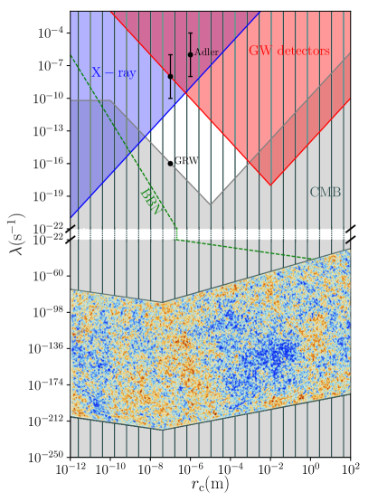
Figure 1: Observational constraints on the two parameters $r_{\mathrm{c}}$ and $\lambda$ of the CSL model obtained in Ref. Martin and Vennin (2019). The white region is allowed by laboratory experiments while the “CMB map” region is allowed by CMB measurements. The green dashed line stands for the upper bound on $\lambda$ if inflation proceeds at the Big-Bang Nucleosynthesis (BBN) scale.

In this section, we briefly discuss the observational status of collapse models in Cosmology. As already mentioned, only few cases have been investigated so far: QMUPL and CSL, both with a white noise and using a naive generalization of non-relativistic collapse models to field theory. A discussion of QMUPL in Cosmology can be found in Refs. Martin et al. (2012); Das et al. (2013) and, here, we focus on CSL since this is the model that has drawn the most attention Martin and Vennin (2019).

The CSL theory consists in assuming that the collapse operator is mass or energy density. In a cosmological context, as already briefly mentioned in the previous section, this corresponds to $\hat{C}=\rho+\widehat{\delta\rho}$, where $\rho$ is the energy density stored in the inflaton field and $\hat{\delta}\equiv\widehat{\delta\rho}/\rho$ is the density contrast. In fact, only the density contrast will be playing a role in what follows because, in inflationary perturbations theory, $\rho$ is a classical quantity and, therefore, cancels out in the modified Schrödinger equation. In General Relativity, however, as already mentioned, there is no unique definition for $\delta$. Nevertheless, see Ref. Martin and Vennin (2019), what matters is in fact the scale dependence of $\delta$, in particular its behavior on large scales. Conveniently, one can show that, for all reasonable choices, all the $\delta$’s behave similarly (namely, in the same way as the Newtonian density contrast “$\delta_{\mathrm{g}}$”) except for one particular case, the so-called “$\delta_{\mathrm{m}}$” density contrast. Therefore, even if the choice of $\delta$ is ambiguous, the final result turns out to be (almost) independent of this choice.

Once the collapse operator has been chosen, one can solve the modified Schrödinger equation and calculate the CSL inflationary power spectrum along the lines explained in the previous sections. This power spectrum depends on the two CSL parameters $\gamma$ and $r_{\mathrm{c}}$. Quite intuitively, one finds that the extra CSL terms operate only if the physical wavelength of a Fourier mode is larger than the localization scale $r_{\mathrm{c}}$. In an expanding universe, physical wavelengths increase with time, so this implies that for any given wavenumber $\bm{k}$, there is a time before which its physical wavelength is smaller than $r_{\mathrm{c}}$, hence the CSL corrections are absent. This is a crucial feature since it guarantees that the usual way of setting initial conditions in the Bunch-Davies vacuum, which is a very important aspect of the inflationary paradigm, is still available.

When the physical wavelength of a Fourier mode becomes larger than $r_{\mathrm{c}}$, the CSL terms become important and collapse occurs. This generates the power spectrum Martin and Vennin (2019)

$${\cal P}_{\zeta}(k) =\frac{k^{3}}{2\pi^{2}}\frac{1}{4\Re\mathrm{e}\,\Omega_{\bm{k}}|_{\gamma=0}}\biggl{[}1+{\cal O}(1)\frac{\gamma}{m_{0}^{2}}\rho\,\epsilon_{1}\left(\frac{r_{\mathrm{c}}}{\ell_{{}_{\rm H}}}\right)_{\rm end}^{\mathfrak{a}}\left(\frac{k}{aH}\right)^{\mathfrak{b}}_{\mathrm{end}}-\frac{\Re\mathrm{e}\,\Omega_{\bm{k}}|_{\gamma=0}}{\Re\mathrm{e}\,\Omega_{\bm{k}}}\biggr{]}.$$ (37)

In the limit where $\gamma=0$, one checks that the power spectrum vanishes, since no perturbation is being produced, in agreement with the discussion presented in Sec. IV. Let us also recall that the “standard” result, obtained in the Copenhagen interpretation, is given by Eq. (18), which matches the prefactor in Eq. (37), and that $\Re\mathrm{e}\,\Omega_{\bm{k}}$ is proportional to the inverse variance of the wave-packet. If $\gamma$ is sufficiently large so that the collapse occurs, the width of the wave-function is much smaller than what it would be in the unmodified theory, hence the third term in the square brackets of Eq. (37) can be neglected when compared to the first term. In that case, the power spectrum takes the form of the standard result, plus a correction proportional to $\gamma$. This CSL correction is also proportional to $\rho\epsilon_{1}$, where $\epsilon_{1}$ is the first slow-roll parameter and $\rho$ the energy density at the end of inflation. Let us recall that, during inflation, $\rho$ is quasi constant and can be as large as

$$\rho\sim 10^{80}\mbox{g}\times\mbox{cm}^{-3}.$$ (38)

We see here why Cosmology is a natural place to probe collapse theories: it tests them in regimes that are completely different, in terms of energy, time or length scales, than those relevant in the lab. Since the amplitude of the CSL new terms are controlled by the energy density, it makes sense to constrain them in physical conditions where $\rho$ is as large as possible. This is why, for instance, the CSL mechanism was also applied to neutron stars in Ref. Tilloy and Stace (2019). Primordial Cosmology is a situation where $\rho$ is even larger and, therefore, one can expect it to be even more appropriate when it comes to establishing constraints on CSL.

The second crucial piece of information that comes from Eq. (37) is that the CSL corrections are not scale invariant. Their scale dependence is $\propto k^{\mathfrak{b}}$ where $\mathfrak{b}=-1$ if the scale $r_{\mathrm{c}}$ is crossed out during inflation and $\mathfrak{b}=-10$ if $r_{\mathrm{c}}$ is crossed out during the subsequent radiation dominated era. In this last case, there is an additional factor $\propto(r_{\mathrm{c}}/\ell_{{}_{\mathrm{H}}})^{\mathfrak{a}}$, where $\ell_{{}_{\mathrm{H}}}$ is the Hubble radius at the end of inflation, with $\mathfrak{a}=-9$ (if $r_{\mathrm{c}}$ is crossed out during inflation, this term is not present and $\mathfrak{a}=0$). In other words, detectable CSL corrections would be strongly incompatible with CMB measurements. Since we have seen that they are typically very large, we expect the constraints that can be inferred from them to be very efficient.

These constraints are represented in Fig. 1 in the space $(r_{\mathrm{c}},\lambda)$ where $\lambda=\gamma/(8\pi^{3/2}r_{\mathrm{c}}^{3})$. In this plot, the white region corresponds to the parameter space allowed by lab experiments while the “CMB map” region corresponds to parameter space allowed by CMB measurements. Evidently, the most striking feature of the plot is that the two regions do not overlap. Taken at face value, this implies that CSL is ruled out! However, this conclusion should be toned down. First, we should notice that if the collapse operator is taken to be $\delta_{\mathrm{m}}$, then the CMB constraints are no longer in contradiction with the lab ones. Of course, in some sense, $\delta_{\mathrm{m}}$ is “of measure zero” in the space of density contrasts but, nevertheless, this shows that one can find collapse operators for which CSL is rescued. Second, one has to remember that we used a naive (too naive?) method to implement the collapse mechanism in field theory. It could be that, when a truly covariant version of collapse models is available Ghirardi et al. (1990); Tumulka (2006); Bedingham (2011); Bedingham et al. (2014), the final result will be modified. For instance, the constraints on the CSL parameters coming from the CMB constraints on one hand, and from lab experiments on the other hand, operate at very different energy scales. One could imagine that, in a field-theoretic context, the CSL parameters run with the energy scale at which the experiment is being performed, and that one cannot simply compare the constraints obtained at different energies. Finally, we used a white noise in the modified Schrödinger equation and it remains to be seen if using a colored noise can modify the constraints obtained in Fig. 1. For all these reasons, it is necessary to be cautious and testing the robustness of the conclusions obtained here will certainly be a major goal in the future.

VI Conclusions

Interestingly enough, collapse models advocated by Giancarlo Ghirardi (and others) and cosmic inflation have almost the same age. Roughly speaking, they were both introduced at the end of the seventies and beginning of the eighties. Nevertheless, until recently, they had never met. In this article, we have described the recent attempts to apply collapse models to inflation. We have argued that there is a good scientific case motivating those attempts. In particular, for collapse models to be interesting and to insure proper localization, the collapse operators must be related to the energy density. As a consequence, the most efficient tests of collapse models will be in physical situations where the energy density is as large as possible. Without any doubt, this is to be found in the early universe. We have shown that, indeed, the high-accuracy data now at our disposal leads to extremely competitive constraints, that anyone interested in collapse theories can no longer ignore. We hope this will cause further investigations to test the robustness of these results.

Finally, after $40$ years, collapse theories and cosmic inflation have met and we are convinced that Giancarlo Ghirardi would have been fascinated by the fact that his great insights about Quantum Mechanics can even find applications in Cosmology.

References

- Bassi et al. (2013) A. Bassi, K. Lochan, S. Satin, T. P. Singh, and H. Ulbricht, Rev. Mod. Phys. 85, 471 (2013), eprint 1204.4325.
- Ghirardi et al. (1986) G. C. Ghirardi, A. Rimini, and T. Weber, Phys. Rev. D34, 470 (1986).
- Pearle (1989) P. M. Pearle, Phys. Rev. A39, 2277 (1989).
- Ghirardi et al. (1990) G. C. Ghirardi, P. M. Pearle, and A. Rimini, Phys. Rev. A42, 78 (1990).
- Bassi and Ghirardi (2003) A. Bassi and G. C. Ghirardi, Phys. Rept. 379, 257 (2003), eprint quant-ph/0302164.
- Esposito-Farese (2004) G. Esposito-Farese, AIP Conf. Proc. 736, 35 (2004), eprint gr-qc/0409081.
- Mukhanov and Chibisov (1981) V. F. Mukhanov and G. Chibisov, JETP Lett. 33, 532 (1981).
- Starobinsky (1980) A. A. Starobinsky, Phys. Lett. B91, 99 (1980).
- Guth (1981) A. H. Guth, Phys. Rev. D23, 347 (1981).
- Linde (1982) A. D. Linde, Phys.Lett. B108, 389 (1982).
- Albrecht and Steinhardt (1982) A. Albrecht and P. J. Steinhardt, Phys. Rev. Lett. 48, 1220 (1982).
- Linde (1983) A. D. Linde, Phys. Lett. B129, 177 (1983).
- von Neumann (1955) J. von Neumann, Mathematical foundations of quantum mechanics (1955).
- Hartle (2019) J. B. Hartle (2019), eprint 1901.03933.
- Bell and Mermin (1988) J. S. Bell and N. D. Mermin, Physics Today 41, 89 (1988).
- Perez et al. (2006) A. Perez, H. Sahlmann, and D. Sudarsky, Class. Quant. Grav. 23, 2317 (2006), eprint gr-qc/0508100.
- Pearle (2007) P. M. Pearle, in Foundational Questions Institute Inaugural Workshop (FQXi 2007 Reykjavik, Iceland, July 21-26, 2007 (2007), eprint 0710.0567.
- Lochan et al. (2012) K. Lochan, S. Das, and A. Bassi, Phys. Rev. D86, 065016 (2012), eprint 1206.4425.
- Martin et al. (2012) J. Martin, V. Vennin, and P. Peter, Phys. Rev. D86, 103524 (2012), eprint 1207.2086.
- Cañate et al. (2013) P. Cañate, P. Pearle, and D. Sudarsky, Phys. Rev. D87, 104024 (2013), eprint 1211.3463.
- Piccirilli et al. (2018) M. P. Piccirilli, G. León, S. J. Landau, M. Benetti, and D. Sudarsky, Int. J. Mod. Phys. D 28, 1950041 (2018), eprint 1709.06237.
- León et al. (2018) G. León, A. Majhi, E. Okon, and D. Sudarsky, Phys. Rev. D 98, 023512 (2018), eprint 1712.02435.
- León et al. (2019) G. León, A. Pujol, S. J. Landau, and M. P. Piccirilli, Phys. Dark Univ. 24, 100285 (2019), eprint 1902.08696.
- Martin and Vennin (2019) J. Martin and V. Vennin (2019), eprint 1906.04405.
- Martin (2019a) J. Martin (2019a), eprint 1902.05286.
- Kodama and Sasaki (1984) H. Kodama and M. Sasaki, Prog. Theor. Phys. Suppl. 78, 1 (1984).
- Ade et al. (2014) P. Ade et al. (Planck), Astron.Astrophys. 571, A16 (2014), eprint 1303.5076.
- Martin et al. (2014a) J. Martin, C. Ringeval, and V. Vennin, Phys. Dark Univ. 5-6, 75–235 (2014a), eprint 1303.3787.
- Martin et al. (2014b) J. Martin, C. Ringeval, R. Trotta, and V. Vennin, JCAP 1403, 039 (2014b), eprint 1312.3529.
- Martin et al. (2015) J. Martin, C. Ringeval, and V. Vennin, Phys. Rev. Lett. 114, 081303 (2015), eprint 1410.7958.
- Martin (2015) J. Martin (2015), eprint 1502.05733.
- Akrami et al. (2018a) Y. Akrami et al. (Planck) (2018a), eprint 1807.06205.
- Akrami et al. (2018b) Y. Akrami et al. (Planck) (2018b), eprint 1807.06211.
- Akrami et al. (2019) Y. Akrami et al. (Planck) (2019), eprint 1905.05697.
- Martin (2008) J. Martin, Lect. Notes Phys. 738, 193 (2008), eprint 0704.3540.
- Cohen-Tannoudji et al. (1992) C. Cohen-Tannoudji, J. Dupont-Roc, and G. Grunberg, Atom - Photon Interactions: Basic Process and Appilcations (Wiley-Interscience, 1992).
- Bunch and Davies (1978) T. Bunch and P. Davies, Proc.Roy.Soc.Lond. A360, 117 (1978).
- Grishchuk and Sidorov (1990) L. Grishchuk and Y. Sidorov, Phys. Rev. D42, 3413 (1990).
- Martin and Vennin (2016a) J. Martin and V. Vennin, Phys. Rev. D93, 023505 (2016a), eprint 1510.04038.
- Grain and Vennin (2019) J. Grain and V. Vennin (2019), eprint 1910.01916.
- Sachs and Wolfe (1967) R. K. Sachs and A. M. Wolfe, Astrophys. J. 147, 73 (1967), [Gen. Rel. Grav.39,1929(2007)].
- Kenfack and Zyczkowski (2004) A. Kenfack and K. Zyczkowski, Journal of Optics B: Quantum and Semiclassical Optics 6, 396 (2004), eprint quant-ph/0406015.
- Polarski and Starobinsky (1996) D. Polarski and A. A. Starobinsky, Class. Quant. Grav. 13, 377 (1996), eprint gr-qc/9504030.
- Albrecht et al. (1994) A. Albrecht, P. Ferreira, M. Joyce, and T. Prokopec, Phys. Rev. D50, 4807 (1994), eprint astro-ph/9303001.
- Revzen (2006) M. Revzen, Foundations of Physics 36, 546 (2006).
- Revzen et al. (2005) M. Revzen, P. A. Mello, A. Mann, and L. M. Johansen, Phys. Rev. A 71, 022103 (2005), eprint quant-ph/0405100.
- Martin and Vennin (2016b) J. Martin and V. Vennin, Phys. Rev. A93, 062117 (2016b), eprint 1605.02944.
- Martin and Vennin (2017) J. Martin and V. Vennin, Phys. Rev. D96, 063501 (2017), eprint 1706.05001.
- Bell (1986) J. S. Bell, Annals of the New York Academy of Sciences 480, 263 (1986).
- Martin (2019b) J. Martin, Universe 5, 92 (2019b), eprint 1904.00083.
- Zurek (1981) W. H. Zurek, Phys. Rev. D24, 1516 (1981).
- Schlosshauer (2004) M. Schlosshauer, Rev. Mod. Phys. 76, 1267 (2004), eprint quant-ph/0312059.
- Burgess et al. (2008) C. P. Burgess, R. Holman, and D. Hoover, Phys.Rev. D77, 063534 (2008), eprint astro-ph/0601646.
- Martin and Vennin (2018a) J. Martin and V. Vennin, JCAP 1805, 063 (2018a), eprint 1801.09949.
- Martin and Vennin (2018b) J. Martin and V. Vennin, JCAP 1806, 037 (2018b), eprint 1805.05609.
- Castagnino et al. (2017) M. Castagnino, S. Fortin, R. Laura, and D. Sudarsky, Found. Phys. 47, 1387 (2017), eprint 1412.7576.
- Tumulka (2006) R. Tumulka, Proc. Roy. Soc. Lond. A462, 1897 (2006), eprint quant-ph/0508230.
- Bedingham (2011) D. J. Bedingham, Found. Phys. 41, 686 (2011), eprint 1003.2774.
- Bedingham et al. (2014) D. Bedingham, D. Dürr, G. Ghirardi, S. Goldstein, R. Tumulka, and N. Zanghì, Journal of Statistical Physics 154, 623 (2014), eprint 1111.1425.
- Schwinger (1951) J. S. Schwinger, Phys. Rev. 82, 664 (1951), [,116(1951)].
- Grishchuk and Martin (1997) L. P. Grishchuk and J. Martin, Phys. Rev. D56, 1924 (1997), eprint gr-qc/9702018.
- Das et al. (2013) S. Das, K. Lochan, S. Sahu, and T. P. Singh, Phys. Rev. D88, 085020 (2013), [Erratum: Phys. Rev.D89,no.10,109902(2014)], eprint 1304.5094.
- Tilloy and Stace (2019) A. Tilloy and T. M. Stace, Phys. Rev. Lett. 123, 080402 (2019), eprint 1901.05477.