Higher order Galerkin–collocation time discretization with Nitsche’s method for the Navier–Stokes equations

Abstract

We propose and study numerically the implicit approximation in time of the Navier–Stokes equations by a Galerkin–collocation method in time combined with inf-sup stable finite element methods in space. The conceptual basis of the Galerkin–collocation approach is the establishment of a direct connection between the Galerkin method and the classical collocation methods, with the perspective of achieving the accuracy of the former with reduced computational costs in terms of less complex algebraic systems of the latter. Regularity of higher order in time of the discrete solution is ensured further. As an additional ingredient, we employ Nitsche’s method to impose all boundary conditions in weak form with the perspective that evolving domains become feasible in the future. We carefully compare the performance poroperties of the Galerkin-collocation approach with a standard continuous Galerkin–Petrov method using piecewise linear polynomials in time, that is algebraically equivalent to the popular Crank–Nicholson scheme. The condition number of the arising linear systems after Newton linearization as well as the reliable approximation of the drag and lift coefficient for laminar flow around a cylinder (DFG flow benchmark with $Re=100$; cf. [51]) are investigated. The superiority of the Galerkin–collocation approach over the linear in time, continuous Galerkin–Petrov method is demonstrated therein.

1 Introduction

In the past, space-time finite element methods with continuous and discontinuous discretizations of the time and space variables have been studied strongly for the numerical simulation of incompressibe flow, wave propagation, transport phenomena or even problems of multi-physics; cf., e.g., [1, 2, 5, 6, 26, 27, 28, 31, 33, 46, 47, 48]. Appreciable advantage of variational space-time discretizations is that they offer the potential to naturally construct higher order methods. In practice, these methods provide accurate results by reasonable numerical costs and on computationally feasible grids. Further, variational space-time discretizations allow to utilize fully adaptive finite element techniques to change the magnitude of the space and time elements in order to increase accuracy and decrease numerical costs; cf. [14, 15, 9]. Strong relations between variational time discretization, collocation and Runge–Kutta methods have been observed [3, 36]. Nodal superconvergence properties of variational time discretizations have also been proved [10].

Recently, a modification of the standard continuous Galerkin–Petrov method (cGP) for the time discretization was introduced for wave problems (cf. [5, 6, 11]). The modification comes through imposing collocation conditions involving the discrete solution’s derivatives at the discrete time nodes while on the other hand reducing the dimension of the test space of the discrete variational problem compared with the standard cGP approach. A further key ingredient is the application of a special Hermite-type quadrature formula, proposed in [32], and interpolation operator for the right-hand side function. Thereby, static condensation of degrees of freedom becomes feasible. These principles offer the potential of achieving the accuracy of Galerkin–Petrov methods with reduced computational costs by less complex algebraic systems. We refer to these schemes as Galerkin–collocation methods. Here, a family of Galerkin–collocation scheme with discrete solutions that are continuously differentiable in time and referred to as GCC¹ schemes is studied only. For families of schemes with even higher regularity in time we refer to [6, 11]. The Galerkin–collocation schemes rely in an essential way on the perfectly matching set of the polynomial spaces (trial and test space), quadrature formula and interpolation operator. For wave problems, the GCC¹ approach has demonstrated its superiority over pure continuous Galerkin–Petrov approximations in time (cGP); cf. [5]. Therefore, it seems to be natural to study the GCC¹ scheme also for the approximation of the Navier–Stokes equations. To the best of our knowledge, this paper is the first work, in that the application of such a Galerkin–collocation scheme to the Navier–Stokes equations is being proposed and investigated.

In the field of computational fluid dynamics, complex and dynamic geometries with moving boundaries are considered often. Fluid-structure interaction is a prominent example of multi-physics for problems with moving boundaries and interfaces. For these problems, Nitsche’s fictitious domain method along with cut finite element techniques has been studied strongly in the recent past; cf. [16, 18, 19, 20, 13, 22, 21, 37, 38, 44] and the references therein. In this approach, the geometry is immersed into an underlying computational grid, which is not fitted to the geometric problem structure and, usually kept fixed over the whole simulation time. Thereby, mesh degeneration and remeshing are avoided for evolving and time-dependent domains. In Nitsche’s method, the Dirichlet boundary conditions are added in a weak form to the variational equation of the partial differential equation, instead of imposing them on the definition of the function spaces of the variational problem.

In this work, the Galerkin–collocation approximation of the Navier–Stokes equations is developed along with Nitsche’s method for imposing Dirichlet boundary conditions. A Newton iteration is applied for solving the resulting nonlinear algebraic system of equations. For the Galerkin–collocation scheme GCC${}^{1}(3)$ with piecewise cubic polynomials the algebraic system along with its Newton linearization is derived explicitly which is done here since the Galerkin–collocation approximation of the Navier–Stokes equations is presented for the first time and to facilitate the traceability of its implementation. The expected convergence behaviour of optimal order in time (and space) is demonstrated for the velocity and pressure variable. For flow around a cylinder it is illustrated that the accuracy of the approximation does not suffer from enforcing the boundary conditions in weak form by the application of Nitsche’s method. Moreover, to show the superiority of the proposed approach over more standard time discretization schemes, a careful comparsion of the GCC${}^{1}(3)$ approach with the continuous Galerkin–Petrov method using piecewise linear polynomials in time is performed. In algebraic form, the latter one can be recovered as the well-known Crank–Nicholson scheme. The errors of both approaches and, with regard to the future construction of efficient iterative solvers, the condition numbers of their Jacobian matrices are evaluated. Further, the performance properties for computing laminar flow around a cylinder are investigated. For this, the well-known DFG flow benchmark with $Re=100$ (cf. [51]) as a challenging flow problem is used. The superiority of the GCC${}^{1}(3)$ approach is cleary observed. Finally, we note that this work is considered as a building block for the future application of the proposed approach to fluid-structure interaction. In our outlook (cf. Sec. 6), the feasibility for flow simulation on dynamically changing domains is demonstrated successfully. Here, a fictitious domain approach and stabilized cut finite element techniques are used; cf. [4].

This paper is organized as follows. In Sec. 2 we introduce our prototype model and notation. In Sec. 3 we present its space-time discretization by Galerkin–collocation methods in time and inf-sup stable pairs of finite elements in space. Nitsche’s method is applied to enforce Dirichlet boundary conditions in a weak sense. In Sec. 4 the Galerkin–collocation scheme GCC${}^{1}(3)$ of piecewise cubic polynomials in time is studied. The algebraic formulation of the discrete system is derived and its solution by Newton’s method is presented. In Sec. 5 a careful numerical study of our approach is provided for the GCC¹(3) member of the Galerkin–collocation schemes. In particular, the condition number of the arising algebraic systems after Newton linearization and the accuracy of the computed drag and lift coefficients for flow around a cylinder with $Re=100$ (DFG benachmark [51]) are compared to the results of a standard cGP approximation with piecewise linear polynomials in time. In Sec. 6, the potential of the presented approach, enriched by cut finite element techniques, for simulating flow on dynamically changing geometries by using fixed background meshes is illustrated.

2 Mathematical problem and notation

2.1 Mathematical problem

To fix our ideas and schemes in a familiar setting and simplify the notation, we restrict ourselves here to a common test problem, that of calculating nonstationary, incompressible flow past an obstacle, here taken as an inclined ellipse situated in a rectangle; cf. Fig. 2.1. A generalization of our approach to more complex and three-dimensional bounded domains is straightforward.

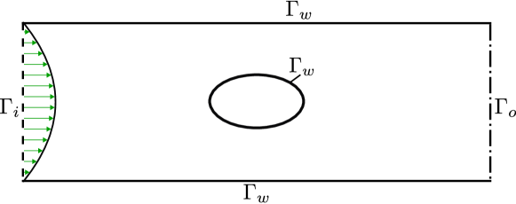
Figure 2.1: Notation for the flow domain $\Omega$.

In this domain $\Omega\subset\mathbb{R}^{2}$ and for the time intervall $I=(0,T]$ we consider solving the Navier–Stokes equations, given in dimensionless form by

$$\partial_{t}\boldsymbol{v}+(\boldsymbol{v}\cdot\nabla)\boldsymbol{v}-\nu\Delta\boldsymbol{v}+\nabla p =\boldsymbol{f} \text{in }\Omega\times I\,,$$ (2.1a)

$$\nabla\cdot\boldsymbol{v} =0 \text{in }\Omega\times I\,,$$ (2.1b)

$$\boldsymbol{v} =\boldsymbol{g} \text{on }\Gamma_{i}\times I\,,$$ (2.1c)

$$\boldsymbol{v} =\boldsymbol{0} \text{on }\Gamma_{w}\times I\,,$$ (2.1d)

$$\nu\nabla\boldsymbol{v}\cdot\boldsymbol{n}-\boldsymbol{n}p =\boldsymbol{0} \text{on }\Gamma_{o}\times I\,,$$ (2.1e)

$$\boldsymbol{v}(0) =\boldsymbol{v}_{0} \text{in }\Omega\,.$$ (2.1f)

In (2.1), the unknows are the velocity field $\boldsymbol{v}$ and the pressure variable $p$. By $\nu$ we denote the dimensionless viscosity. Further, $\boldsymbol{f}$ is a given external force, $\boldsymbol{v}_{0}$ is the initial velocity and $\boldsymbol{g}$ is the prescribed velocity at the inflow boundary $\Gamma_{i}$. Eq. (2.1e) is the so-called do-nothing boundary condition for the outflow boundary $\Gamma_{o}$ with the outer unit normal vector $\boldsymbol{n}=\boldsymbol{n}(\boldsymbol{x})$; cf. [30]. At the upper and lower walls and on the boundary of the ellipse, jointly refered to as $\Gamma_{w}$, the no-slip boundary condition (2.1d) is used. For short, we put $\Gamma:=\Gamma_{i}\cup\Gamma_{w}\cup\Gamma_{o}$ and $\Gamma_{D}:=\Gamma_{i}\cup\Gamma_{w}$.

Wellposedness of the Navier–Stokes equations (2.1) and the existence of weak, strong or regular solutions to (2.1) in two and three space dimensions is not discussed here. The same applies to the optimal regularity of Navier–Stokes solutions at $t=0$ and the existence of non-local compatibility conditions. For the comprehensive discussion of these topics, we refer to the wide literature in this field; cf., e.g., [30, 42, 49] as well as [8, 41] and the references therein. Here, we assume the existence of a sufficiently regular (local) solution to the initial-boundary value problem (2.1) such that higher-order time and space discretizations become feasible. In particular we tacitly suppose that the solution to (2.1) is sufficient regular such that all of the equations given below are well-defined.

2.2 Notation

In this work we use standard notation. $H^{m}(\Omega)$ is the Sobolev space of $L^{2}(\Omega)$ functions with derivatives up to order $m$ in $L^{2}(\Omega)$ and by $\langle\cdot,\cdot\rangle$ the inner product in $L^{2}(\Omega)$ and $(L^{2}(\Omega))^{2}$, respectively. In the notation of the inner product we do not differ between the scalar- and vector-valued case. Throughout, the meaning will be obvious from the context. We let

$$H^{1}_{0,\Gamma_{D}}(\Omega):=\{u\in H^{1}(\Omega)\mid u=0\mbox{ on }\Gamma_{D}=\Gamma_{i}\cup\Gamma_{w}\}\,.$$

For short, we put

$$Q:=L^{2}(\Omega)\,,\quad\boldsymbol{V}:=\left(H^{1}(\Omega)\right)^{2}\,,\quad\boldsymbol{V}_{0}:=\left(H^{1}_{0,\Gamma_{D}}(\Omega)\right)^{2}$$

and

$$\boldsymbol{X}=\boldsymbol{V}\times Q\,,\quad\boldsymbol{X}_{0}:=\boldsymbol{V}_{0}\times Q\,.$$

Further, we define the function spaces

$$\boldsymbol{V}_{\text{div}}:=\{\boldsymbol{u}\in\boldsymbol{V}\mid\nabla\cdot\boldsymbol{u}=0\}\quad\text{and}\quad\boldsymbol{V}^{0}_{\text{div}}=\boldsymbol{V}_{\text{div}}\cap\boldsymbol{V}_{0}\,.$$

We denote by $\boldsymbol{V}^{\prime}$ the dual space of $\boldsymbol{V}_{0}$.

For a Banach space $B$, we let $L^{2}(0,T;B)$, $C([0,T];B)$, and $C^{m}([0,T];B)$, $m\in\mathbb{N}$, be the Bochner spaces of $B$-valued functions, equipped with their natural norms. For a subinterval $J\subseteq[0,T]$, we use the notations $L^{2}(J;B)$, $C^{m}(J;B)$, and $C^{0}(J;B):=C(J;B)$.

For the time discretization, we decompose the time interval $I=(0,T]$ into $N$ subintervals $I_{n}=(t_{n-1},t_{n}]$, $n=1,\ldots,N$, where $0=t_{0}<t_{1}<\cdots<t_{N-1}<t_{N}=T$ such that $I=\bigcup_{n=1}^{N}I_{n}$. We put $\tau=\max_{n=1,\ldots,N}\tau_{n}$ with $\tau_{n}=t_{n}-t_{n-1}$. Further, the set $\mathcal{M}_{\tau}:=\{I_{1},\ldots,I_{N}\}$ of time intervals is called the time mesh. For a Banach space $B$ and any $k\in\mathbb{N}_{0}$, we let

$$\mathbb{P}_{k}(I_{n};B)=\Big{\{}w_{\tau}:I_{n}\to B\mid w_{\tau}(t)=\mbox{$\sum\limits_{j=0}^{k}$}W^{j}t^{j}\;\forall t\in I_{n}\,,\;W^{j}\in B\;\forall j\Big{\}}\,.$$

For an integer $k\in\mathbb{N}$, we introduce the space

$$X_{\tau}^{k}(B):=\left\{w_{\tau}\in C(\overline{I};B)\mid w_{\tau}|_{I_{n}}\in\mathbb{P}_{k}(I_{n};B)\;\forall I_{n}\in\mathcal{M}_{\tau}\right\}$$

of globally continuous functions in time and for an integer $l\in\mathbb{N}_{0}$ the space

$$Y_{\tau}^{l}(B):=\left\{w_{\tau}\in L^{2}(I;B)\mid w_{\tau}|_{I_{n}}\in\mathbb{P}_{l}(I_{n};B)\;\forall I_{n}\in\mathcal{M}_{\tau}\right\}$$

of global $L^{2}$-functions in time. For the space discretization, let $\mathcal{T}_{h}$ be a shape-regular mesh of $\Omega$ consisting of quadrilateral elements with mesh size $h>0$. For some $r\in\mathbb{N}$, let $H_{h}=H_{h}^{(r)}$ be the finite element space given by

$$H_{h}^{(r)}=\left\{v_{h}\in C(\overline{\Omega})\mid v_{h}{}|_{T}\in\mathbb{Q}_{r}(K)\,\forall K\in\mathcal{T}_{h}\right\}\,,$$ (2.2)

where $\mathbb{Q}_{r}(K)$ is the space defined by the multilinear reference mapping of polynomials on the reference element with maximum degree $r$ in each variable. For brevity, we restrict our presentation to the Taylor–Hood family of inf-sup stable finite element pairs for the space discretization. The elements are used in the numerical experiments that are presented in Sec. 5. However, these elements can be replaced by any other type of inf-sup stable elements. For some natural number $r\geq 2$ and with (2.2) we then put

$$V_{h}=H_{h}^{(r)}\,,\quad V_{h}^{0}=H_{h}^{(r)}\cap H^{1}_{0,\Gamma_{D}}(\Omega)\,,\quad Q_{h}=H_{h}^{(r-1)}$$

and

$$X_{h}:=V_{h}\times Q_{h}\,,\quad X_{h}^{0}:=V_{h}^{0}\times Q_{h}\,,$$

as well as

$$\boldsymbol{V}_{h}=(V_{h})^{2}\,,\quad\boldsymbol{V}_{h}^{0}=(V_{h}^{0})^{2}\,,\quad\boldsymbol{X}_{h}=\boldsymbol{V}_{h}\times Q_{h}\,,\quad\boldsymbol{X}_{h}^{0}=\boldsymbol{V}_{h}^{0}\times Q_{h}\,.$$

The space of weakly divergence free functions is denoted by

$$\boldsymbol{V}_{h}^{\text{div}}=\{\boldsymbol{v}_{h}\in\boldsymbol{V}_{h}\mid\langle\nabla\cdot\boldsymbol{v}_{h},q_{h}\rangle=0\;\text{for all }q_{h}\in Q_{h}\}\,.$$

For the discrete space-time functions spaces we use the abbreviations

$$\boldsymbol{X}^{k}_{\tau,h}=(X_{\tau}^{k}(V_{h}))^{2}\times X_{\tau}^{k}(Q_{h})\,,\quad\boldsymbol{Y}^{k}_{\tau,h}=(Y_{\tau}^{k}(V_{h}))^{2}\times Y_{\tau}^{k}(Q_{h})$$

and

$$\boldsymbol{X}^{k,0}_{\tau,h}=(X_{\tau}^{k}(V_{h}^{0}))^{2}\times X_{\tau}^{k}(Q_{h})\,,\quad\boldsymbol{Y}^{k,0}_{\tau,h}=(Y_{\tau}^{k}(V_{h}^{0}))^{2}\times Y_{\tau}^{k}(Q_{h})$$

Further, we define the semi-linear form $a:\boldsymbol{X}\times\boldsymbol{X}\rightarrow\mathbb{R}$ by

$$a(\boldsymbol{u},\boldsymbol{\phi}) :=\langle\partial_{t}\boldsymbol{v},\boldsymbol{\psi}\rangle+\langle(\boldsymbol{v}\cdot\boldsymbol{\nabla})\boldsymbol{v},\boldsymbol{\psi}\rangle+\nu\langle\nabla\boldsymbol{v},\nabla\boldsymbol{\psi}\rangle-\langle p,\nabla\cdot\boldsymbol{\psi}\rangle+\langle\boldsymbol{\nabla}\cdot\boldsymbol{v},\xi\rangle$$ (2.3)

for $\boldsymbol{u}=(\boldsymbol{v},p)\in\boldsymbol{X}$ and $\boldsymbol{\phi}=(\boldsymbol{\psi},\xi)\in\boldsymbol{X}$ and the linear form $L:\boldsymbol{X}\rightarrow\mathbb{R}$ by

$$L(\boldsymbol{\phi};\boldsymbol{f}):=\langle\boldsymbol{f},\boldsymbol{\psi}\rangle$$

for $\boldsymbol{\phi}=(\boldsymbol{\psi},\xi)\in\boldsymbol{X}$. For some parameters $\gamma_{1}>0$ and $\gamma_{2}>0$ (to be discussed below) and

$$(\boldsymbol{v}\cdot\boldsymbol{n})^{-}:=\left\{\begin{array}[]{@{}ll}\boldsymbol{v}\cdot\boldsymbol{n}&\text{if}\;\;\boldsymbol{v}\cdot\boldsymbol{n}<0\,,\\[4.30554pt] 0&\text{else}\,,\end{array}\right.$$

we introduce the semi-linear form $b:\boldsymbol{H}^{1/2}(\Gamma_{D})\times\boldsymbol{X}_{h}\rightarrow\mathbb{R}$ by

$$b_{\gamma}(\boldsymbol{w},\boldsymbol{\phi}_{h}):= -\langle\boldsymbol{w},\nu\nabla\boldsymbol{\psi}_{h}\cdot\boldsymbol{n}+\xi_{h}\boldsymbol{n}\rangle_{\Gamma_{D}}-\langle(\boldsymbol{w}\cdot\boldsymbol{n})^{-}\boldsymbol{w},\boldsymbol{\psi}_{h}\rangle_{\Gamma_{D}}$$ (2.4)

$$\quad+\gamma_{1}\nu\langle h^{-1}\boldsymbol{w},\boldsymbol{\psi}_{h}\rangle_{\Gamma_{D}}+\gamma_{2}\langle h^{-1}\boldsymbol{w}\cdot\boldsymbol{n},\boldsymbol{\psi}_{h}\cdot\boldsymbol{n}\rangle_{\Gamma_{D}}$$

for $\boldsymbol{w}\in\boldsymbol{H}^{1/2}(\Gamma_{D})$ and $\boldsymbol{\phi}_{h}=(\boldsymbol{\psi}_{h},\xi_{h})\in\boldsymbol{X}_{h}$. Finally, with (2.3) and (2.4) the semi-linear form $a_{\gamma}:\boldsymbol{X}_{h}\times\boldsymbol{X}_{h}\rightarrow\mathbb{R}$ is given by

$$a_{\gamma}(\boldsymbol{u}_{h},\boldsymbol{\phi}_{h}):=a(\boldsymbol{u}_{h},\boldsymbol{\phi}_{h})-\langle\nu\nabla\boldsymbol{v}_{h}\cdot\boldsymbol{n}-p_{h}\boldsymbol{n},\boldsymbol{\psi}_{h}\rangle_{\Gamma_{D}}+b_{\gamma}(\boldsymbol{v}_{h},\boldsymbol{\phi}_{h})$$ (2.5)

for $\boldsymbol{u}_{h}=(\boldsymbol{v}_{h},p_{h})\in\boldsymbol{X}_{h}$ and $\boldsymbol{\phi}_{h}=(\boldsymbol{\psi}_{h},\xi_{h})\in\boldsymbol{X}_{h}$.

3 Space-time finite element discretization with Galerkin–collocation time discretization and Nitsche’s method

In this work, Nitsche’s method [39] is applied within a space-time finite element discretization. In contrast to more standard formulations, the Dirichlet boundary conditions for the velocity field (2.1c) and (2.1d) are enforced weakly in the variational equation in terms of line integrals (surface integrals in three space dimensions). Our motivation for applying Nitsche’s method comes through developing here a building block for flow problems with immersed or moving boundaries or even fluid-structure interaction that is based on using non-fitted background finite element meshes along with cut finite element techniques; cf. Sec. 6. For the time discretization a continuous Galerkin–Petrov approach (cf., e.g., [26, 27, 28]) with discrete solutions $\boldsymbol{v}_{\tau,h}\in(C([0,T];X_{h}))^{2}$ and $p\in C([0,T];Q_{h})$ is modified to a Galerkin–collocation approximation by combining the Galerkin techniques with the concepts of collocation. This approach has recently been developed [5] and studied by an error analysis [6] for wave equations. For this type of problems, the Galerkin–collocation approach has demonstrated its superiority over a pure Galerkin approach such that is seems to be worthwhile to apply the Galerkin–collocation technique also to the Navier–Stokes system (2.1).

3.1 Space-time finite element discretization with Nitsche’s fictious domain method

A sufficiently regular solution of the Navier–Stokes system (2.1) satisfies the following variational space-time problem.

Problem 3.1 (Variational space-time problem).

Let $\boldsymbol{v}_{0}\in\boldsymbol{V}_{\operatorname{div}}$ be given. Let $\boldsymbol{\widehat{g}}\in\boldsymbol{V}_{\operatorname{div}}$ denote a prolongation of $\boldsymbol{g}$ such that $\boldsymbol{\widehat{g}}=\boldsymbol{g}$ on $\Gamma_{i}$ and $\boldsymbol{\widehat{g}}=\boldsymbol{0}$ on $\Gamma_{w}$. Put $\boldsymbol{\widehat{u}}=(\boldsymbol{\widehat{g}},0)$. Let $\boldsymbol{f}\in L^{2}(0,T;\boldsymbol{V}^{\prime})$ be given. Find $\boldsymbol{u}\in\boldsymbol{\widehat{u}}+L^{2}(0,T;\boldsymbol{X}_{0})$ such that $\boldsymbol{v}(0)=\boldsymbol{v}_{0}$ and

$$\int_{0}^{T}a(\boldsymbol{u},\boldsymbol{\phi})\;\mathrm{d}t=\int_{0}^{T}L(\boldsymbol{\phi};\boldsymbol{f})\;\mathrm{d}t$$

for all $\boldsymbol{\phi}\in L^{2}(0,T;\boldsymbol{X}_{0})$

For completeness and comparison, we briefly present the standard continuous Galerkin–Petrov approximation in time of Problem 3.1, refered to as cGP($k$), along with the space discretization space; cf., e.g., [26, 27, 28]. This reads as follows.

Problem 3.2 (Global problem of cGP($k$)).

Let an approximation $\boldsymbol{v}_{0,h}\in\boldsymbol{V}_{h}^{\operatorname{div}}$ of the initial value $\boldsymbol{v}_{0}$ be given. Let $\boldsymbol{\widehat{g}}_{\tau,h}\in\boldsymbol{X}^{k}_{\tau,h}$ denote a prolongation in the finite element spaces of the Dirichlet conditions on $\Gamma_{i}$ and $\Gamma_{w}$ . Put $\boldsymbol{\widehat{u}}_{\tau,h}=(\boldsymbol{\widehat{g}_{\tau,h}},0)$. Let $\boldsymbol{f}\in L^{2}(0,T;\boldsymbol{V}^{\prime})$ be given. Find $\boldsymbol{u}_{\tau,h}\in\boldsymbol{\widehat{u}}_{\tau,h}+\boldsymbol{X}^{k,0}_{\tau,h}$ such that $\boldsymbol{v}_{\tau,h}(0)=\boldsymbol{v}_{0,h}$ and

$$\int_{0}^{T}a(\boldsymbol{u}_{\tau,h},\boldsymbol{\phi}_{\tau,h})\;\mathrm{d}t=\int_{0}^{T}L(\boldsymbol{\phi}_{\tau,h};\boldsymbol{f})\;\mathrm{d}t$$

for all $\boldsymbol{\phi}_{\tau,h}\in\boldsymbol{Y}^{k-1,0}_{\tau,h}$.

By choosing test functions in $\boldsymbol{Y}^{k-1,0}_{\tau,h}$ supported on a single subinterval $I_{n}$ of the time mesh $\mathcal{M}_{\tau}$ we recast Problem 3.2 as a time-marching scheme that is given by the following sequence of local problems on the subintervals $I_{n}$.

Problem 3.3 (Local problem of cGP($k$)).

Let an approximation $\boldsymbol{v}_{0,h}\in\boldsymbol{V}_{h}^{\operatorname{div}}$ of the initial value $\boldsymbol{v}_{0}$ be given. Let $\boldsymbol{\widehat{g}}_{\tau,h}\in\boldsymbol{X}^{k}_{\tau,h}$ denote a prolongation into the finite element space of the Dirichlet conditions on $\Gamma_{i}$ and $\Gamma_{w}$ . Put $\boldsymbol{\widehat{u}}_{\tau,h}=(\boldsymbol{\widehat{g}_{\tau,h}},0)$. Let $\boldsymbol{f}\in L^{2}(0,T;\boldsymbol{V}^{\prime})$ be given. For $n=1,\ldots,N$ and given $\boldsymbol{u}_{\tau,h}{}_{|I_{n-1}}\in\boldsymbol{\widehat{u}}_{\tau,h}+(\mathbb{P}_{k}(I_{n-1};V_{h}^{0}))^{2}\times\mathbb{P}_{k}(I_{n-1};Q_{h})$ find $\boldsymbol{u}_{\tau,h}{}_{|I_{n}}\in\boldsymbol{\widehat{u}}_{\tau,h}+(\mathbb{P}_{k}(I_{n};V_{h}^{0}))^{2}\times\mathbb{P}_{k}(I_{n};Q_{h})$ such that

$$\boldsymbol{v}_{\tau,h}{}_{|I_{n}}(t_{n-1}) =\boldsymbol{v}_{\tau,h}{}_{|I_{n-1}}(t_{n-1})\,,$$

$$p_{\tau,h}{}_{|I_{n}}(t_{n-1}) =p_{\tau,h}{}_{|I_{n-1}}(t_{n-1})$$

and

$$\int_{I_{n}}a(\boldsymbol{u}_{\tau,h},\boldsymbol{\phi}_{\tau,h})\;\mathrm{d}t=\int_{I_{n}}L(\boldsymbol{\phi}_{\tau,h};\boldsymbol{f})\;\mathrm{d}t$$ (3.2)

for all $\boldsymbol{\phi}_{\tau,h}\in(\mathbb{P}_{k-1}(I_{n};V_{h}^{0}))^{2}\times\mathbb{P}_{k-1}(I_{n};Q_{h})$.

In practice, the integral on the right-hand side of (3.2) is evaluated by means of an appropriate quadrature formula; cf. [10, 26, 27, 28].

Remark 1 (Definition of initial pressure).

• In Problem  3.3, the quantities $\boldsymbol{v}_{\tau,h}{}_{|I_{n-1}}(t_{n-1})$ and $p_{\tau,h}{}_{|I_{n-1}}(t_{n-1})$ still need to be defined for $n=1$. For the velocity field we put $\boldsymbol{v}_{\tau,h}{}_{|I_{n-1}}(t_{n-1}):=\boldsymbol{v}_{0,h}$ for $n=1$ and with the approximation $\boldsymbol{v}_{0,h}$ of the initial value $\boldsymbol{v}_{0}$. Thus, it remains to define an approximation $p_{0,h}$ of the initial pressure $p_{0}:=p(0)$. This problem is more involved since the Navier–Stokes system does not provide an initial pressure. It is also impacted by the choice of the quadrature formula and the nodal interpolation properties of the temporal basis functions. A remedy based on Gauss quadrature in time and a post-processing for higher order pressure values in the discrete time nodes is proposed in [26, 28]. A further remedy consists in the application of a discontinuous Galerkin approximation (cf. [28]) for the initial time step. In [45], a modification of the Crank–Nicholson scheme that is (up to quadrature) algebraically equivalent to the cGP(1) scheme is proposed by replacing the first two time steps with two implicit Euler steps. Regularity results for the Stokes equations, ensuring the optimal second order of convergence for the Crank–Nicholson scheme, are also studied in [52]. Nevertheless, this topic demands further research.

• If the Navier–Stokes problem (2.1) is considered with (homogeneous) Dirichlet boundary conditions only, the unknown initial pressure $p_{0}:=p(0)\in L^{2}_{0}(\Omega)$ satisfies the boundary value probem (cf. [30, p. 376], [25])

  $$-\Delta p_{0} =-\nabla\cdot\boldsymbol{f}(0)+\nabla\cdot((\boldsymbol{v}_{0}\cdot\nabla)\boldsymbol{v}_{0}) \text{in }\;\Omega\,,$$ (3.3a)

  $$\nabla p_{0}\cdot\boldsymbol{n} =\big{(}\boldsymbol{f}(0)+\nu\Delta\boldsymbol{v}_{0}\big{)}\cdot\boldsymbol{n} \text{on }\;\partial\Omega\,.$$ (3.3b)

  In this case, we put $p_{\tau,h}{}_{|I_{n-1}}(t_{n-1}):=p_{0,h}$ for $n=1$ where $p_{0,h}\in Q_{h}\cap L^{2}_{0}(\Omega)$ denotes a finite element approximation of the solution $p(0)$ to (3.3).

In the variational equation (3.2), Dirichlet boundary conditions for the velocity field are enforced by the definition of the function space $(\mathbb{P}_{k}(I_{n};V_{h}^{0}))^{2}$ where by the discrete space $(V_{h}^{0})^{2}$ homogeneous Dirichlet boundary conditions are prescribed for the velocity approximation $\boldsymbol{v}_{\tau,h}-\boldsymbol{\widehat{g}}_{\tau,h}$ and the test function $\boldsymbol{\psi}_{\tau,h}$. Using the Nitsche method, we solve instead of Problem 3.2 the following one to that we refer to as cGP($k$)–N.

Problem 3.4 (Local Nitsche problem of cGP($k$): cGP($k$)–N).

Let an approximation $\boldsymbol{v}_{0,h}\in\boldsymbol{V}_{h}^{\operatorname{div}}$ of the initial value $\boldsymbol{v}_{0}$ be given. For $n=1,\ldots,N$ and given $\boldsymbol{u}_{\tau,h}{}_{|I_{n-1}}\in(\mathbb{P}_{k}(I_{n-1};V_{h}))^{2}\times\mathbb{P}_{k}(I_{n-1};Q_{h})$ find $\boldsymbol{u}_{\tau,h}{}_{|I_{n}}\in(\mathbb{P}_{k}(I_{n};V_{h}))^{2}\times\mathbb{P}_{k}(I_{n};Q_{h})$ such that

$$\boldsymbol{v}_{\tau,h}{}_{|I_{n}}(t_{n-1}) =\boldsymbol{v}_{\tau,h}{}_{|I_{n-1}}(t_{n-1})\,,$$ (3.4)

$$p_{\tau,h}{}_{|I_{n}}(t_{n-1}) =p_{\tau,h}{}_{|I_{n-1}}(t_{n-1})$$

and

$$\int_{I_{n}}a_{\gamma}(\boldsymbol{u}_{\tau,h},\boldsymbol{\phi}_{\tau,h})\;\mathrm{d}t=\int_{I_{n}}(L(\boldsymbol{\phi}_{\tau,h};\boldsymbol{f})+b_{\gamma}(\boldsymbol{g},\boldsymbol{\phi}_{\tau,h}))\;\mathrm{d}t$$ (3.5)

for all $\boldsymbol{\phi}_{\tau,h}\in(\mathbb{P}_{k-1}(I_{n};V_{h}))^{2}\times\mathbb{P}_{k-1}(I_{n};Q_{h})$.

In Problem 3.5, the Dirichlet boundary conditions for the velocity approximation are now ensured by the contribution of $b_{\gamma}$ to $a_{\gamma}$ and to the right-hand side of (3.5). For the definition of $a_{\gamma}$ and $b_{\gamma}$ we refer to (2.5) and (2.4), respectively. Let us still comment on the different boundary terms (line integrals in two dimensions and surface integrals in three dimensions) in the semi-linear forms (2.5) and (2.4). The second term on the right-hand side of (2.5) reflects the natural boundary condition, making the method consistent. The terms in $b_{\gamma}$ admit the following interpretation. The first term on the right-hand side of (2.4) is introduced to preserve the symmetry properties of the continuous system. The second term incorporates the inflow condition. The last two term are penalty terms that insure the stability of the discrete system. In the inviscid limit $\nu=0$, the last term amounts to a ”no-penetration” condition. Thus, the semi-linear form $b_{\gamma}$ provides a natural weighting between boundary terms corresponding to viscous effects ($\boldsymbol{v}=\boldsymbol{g}$), convective behaviour ($(\boldsymbol{v}\cdot\boldsymbol{n})^{-}\boldsymbol{v}=(\boldsymbol{g}\cdot\boldsymbol{n})^{-}\boldsymbol{g}$) and inviscid behaviour ($\boldsymbol{v}\cdot\boldsymbol{n}=\boldsymbol{g}\cdot\boldsymbol{n}$). Since the second term on the right-hand side of (2.4) introduces a further nonlinearity, this term with little influence is ignored in the case of low Reynolds number flow that is assumed here (cf. Sec. 5).

3.2 Galerkin–collocation time discretization

Our modification of the standard continuous Galerkin–Petrov method (cGP) for time discretization, that is used in Problem 3.3, and the innovation of this work comes through imposing a collocation condition involving the discrete solution’s first derivative at the endpoint of the subinterval $I_{n}$ along with $C^{1}$-continuity constraints at the initial point of the subinterval $I_{n}$ while on the other hand downsizing the test space of the variational equation (3.2). This principle is applied with the perspective of achieving the accuracy of Galerkin schemes with reduced computational costs. We refer to this family of schemes combining Galerkin and collocation techniques as Galerkin–collocation methods, for short GCC¹($k$), where $k$ denotes the degree of the piecewise polynomial approximation in time and the part C¹ in GCC¹($k$) denotes the continuous differentiability of the discrete solution. A further key ingredient in the construction of the Galerkin–collocation approach comes through the application of a special quadrature formula, investigated in [32], and the definition of a related interpolation operator for the right-hand side term of the variational equation. Both of them use derivatives of the given function. The Galerkin–collocation schemes rely in an essential way on the perfectly matching set of the polynomial spaces (trial and test space), quadrature formula, and interpolation operator. In particular, a condensation of degrees of freedom becomes feasibel by the construction principle such that smaller algebraic systems are obtained. The concept of Galerkin–collocation approximation was recently introduced in [11] for systems of ordinary differential equations and applied successfully to wave problems in [5, 6]. Besides the numerical studies given in [5], showing the superiority of the Galerkin-collocation approach over a pure Galerkin approach as used in Problem 3.3, a rigorous error analysis is provided for the Galerkin–collocation approximation of wave phenomena in [6].

From now on we assume a polynomial degree of $k\geq 3$. To introduce the Galerkin–collocation approximation, we need to define the Hermite quadrature formula and the corresponding interpolation operator. Let $\hat{t}^{\,\mathrm{H}}_{1}=-1$, $\hat{t}^{\,\mathrm{H}}_{k-1}=1$, and $\hat{t}^{\,\mathrm{H}}_{s}$, $s=2,\dots,k-2$, be the roots of the Jacobi polynomial on $\widehat{I}:=[-1,1]$ with degree $k-3$ associated to the weighting function $(1-\hat{t})^{2}(1+\hat{t})^{2}$. Let $\widehat{I}^{\,\mathrm{H}}:C^{1}\big{(}\widehat{I};B\big{)}\to\mathbb{P}_{k}\big{(}\widehat{I};B\big{)}$ denote the Hermite interpolation operator with respect to point value and first derivative at both $-1$ and $1$ as well as the point values at $\hat{t}_{s}^{\,\mathrm{H}}$, $s=2,\dots,k-2$. By

$$\widehat{Q}^{\mathrm{H}}(\hat{g}):=\int_{-1}^{1}\widehat{I}^{\,\mathrm{H}}(\hat{g})(\hat{t})\;\mathrm{d}\hat{t}$$

we define an Hermite-type quadrature on $[-1,1]$ which can be written as

$$\widehat{Q}^{\mathrm{H}}(\hat{g})=\widehat{\omega}_{L}\hat{g}^{\prime}(-1)+\sum_{s=1}^{k-1}\widehat{\omega}_{s}\hat{g}(\hat{t}^{\,\mathrm{H}}_{s})+\widehat{\omega}_{R}\hat{g}^{\prime}(1)\,,$$

where all weights are non-zero. Using the affine mapping $T_{n}:\widehat{I}\to\overline{I}_{n}$ with $T_{n}(-1)=t_{n-1}$ and $T_{n}(1)=t_{n}$, we obtain

$$Q_{n}^{\mathrm{H}}(g)=\left(\frac{\tau_{n}}{2}\right)^{2}\widehat{\omega}_{L}\;\mathrm{d}_{t}g(t_{n-1}^{+})+\frac{\tau_{n}}{2}\sum_{s=1}^{k-1}\widehat{\omega}_{s}g(t^{\mathrm{H}}_{n,s})+\left(\frac{\tau_{n}}{2}\right)^{2}\widehat{\omega}_{R}\;\mathrm{d}_{t}g(t_{n}^{-})$$ (3.6)

as Hermite-type quadrature formula on $I_{n}$, where $t^{\mathrm{H}}_{n,s}:=T_{n}(\hat{t}^{\mathrm{H}}_{s})$, $s=1,\dots,k-1$. We note that $Q_{n}^{\mathrm{H}}$ as defined by (3.6) integrates all polynomials up to degree $2k-3$ exactly, cf. [32]. Using $\widehat{I}^{\,\mathrm{H}}$ and $T_{n}$, the local Hermite interpolation on $I_{n}$ is given by

$$I_{n}^{\mathrm{H}}:C^{1}(\overline{I}_{n};B)\to\mathbb{P}_{k}(\overline{I}_{n};B)\,,\qquad v\mapsto\big{(}\widehat{I}^{\,\mathrm{H}}(v\circ T_{n})\big{)}\circ T_{n}^{-1}\,.$$ (3.7)

Moreover, for all $n=1,\dots,N$ we define the global Hermite interpolation $I_{\tau}^{\mathrm{H}}:C^{1}(\overline{I};B)\to X_{\tau}^{k}(B)$ by means of

$$I_{\tau}^{\mathrm{H}}w|_{I_{n}}:=I_{n}^{\mathrm{H}}(w|_{I_{n}})\,.$$ (3.8)

This operator is applied componentwise to vector-valued functions.

The local problem of the Galerkin–collocation approach along with Nitsche’s method for enforcing Dirichlet boundary conditions then reads as follows.

Problem 3.5 (Local $I_{n}$ problem of GCC¹($k$) with Nitsche’s method: GCC¹($k$)–N).

Let $k\geq 3$ and an approximation $\boldsymbol{v}_{0,h}\in\boldsymbol{V}_{h}^{\operatorname{div}}$ of the initial value $\boldsymbol{v}_{0}$ be given. For $n=1,\ldots,N$ and given $\boldsymbol{u}_{\tau,h}{}_{|I_{n-1}}\in(\mathbb{P}_{k}(I_{n-1};V_{h}))^{2}\times\mathbb{P}_{k}(I_{n-1};Q_{h})$ find $\boldsymbol{u}_{\tau,h}{}_{|I_{n}}\in(\mathbb{P}_{k}(I_{n};V_{h}))^{2}\times\mathbb{P}_{k}(I_{n};Q_{h})$ such that

$$\boldsymbol{v}_{\tau,h}{}_{|I_{n}}(t_{n-1}) =\boldsymbol{v}_{\tau,h}{}_{|I_{n-1}}(t_{n-1})\,, \partial_{t}\boldsymbol{v}_{\tau,h}{}_{|I_{n}}(t_{n-1}) =\partial_{t}\boldsymbol{v}_{\tau,h}{}_{|I_{n-1}}(t_{n-1})\,,$$ (3.9)

$$p_{\tau,h}{}_{|I_{n}}(t_{n-1}) =p_{\tau,h}{}_{|I_{n-1}}(t_{n-1})\,, \partial_{t}p_{\tau,h}{}_{|I_{n}}(t_{n-1}) =\partial_{t}p_{\tau,h}{}_{|I_{n-1}}(t_{n-1})\,,$$ (3.10)

and

$$a_{\gamma}(\boldsymbol{u}_{\tau,h}(t_{n}),\boldsymbol{\phi}_{h})=L(\boldsymbol{\phi}_{h};I_{\tau}^{\mathrm{H}}\boldsymbol{f}(t_{n}))+b_{\gamma}(I_{\tau}^{\mathrm{H}}\boldsymbol{g}(t_{n}),\boldsymbol{\phi}_{h})$$ (3.11)

for all $\boldsymbol{\phi}_{h}\in\boldsymbol{X}_{h}$ as well as

$$\int_{I_{n}}a_{\gamma}(\boldsymbol{u}_{\tau,h},\boldsymbol{\phi}_{\tau,h})\;\mathrm{d}t=\int_{I_{n}}(L(\boldsymbol{\phi}_{\tau,h};I_{\tau}^{\mathrm{H}}\boldsymbol{f})+b_{\gamma}(I_{\tau}^{\mathrm{H}}\boldsymbol{g},\boldsymbol{\phi}_{\tau,h}))\;\mathrm{d}t$$ (3.12)

for all $\boldsymbol{\phi}_{\tau,h}\in(\mathbb{P}_{k-3}(I_{n};V_{h}))^{2}\times\mathbb{P}_{k-3}(I_{n};Q_{h})$.

Remark 2.

• In Problem 3.5 the variational equation (3.12) is combined with the collocation condition (3.11) at the endpoint $t_{n}$ of $I_{n}$ and the continuity constraints (3.9), (3.10).

• By definition (3.8) of the Hermite-type interpolation operator $I_{\tau}^{\mathrm{H}}$, we have that $\partial_{t}^{s}I_{\tau}^{\mathrm{H}}\boldsymbol{f}(t_{n})=\partial_{t}^{s}\boldsymbol{f}(t_{n})$ and $\partial_{t}I_{\tau}^{\mathrm{H}}\boldsymbol{g}(t_{n})=\partial_{t}\boldsymbol{g}(t_{n})$ for $s\in\{0,1\}$ on the right-hand side of (3.11).

• The choice of the temporal basis (cf. Eqs. (4.8), that is induced by the definition of the Hermite-type quadrature formula (3.9) and the interpolation operator definition (3.8), allows a computationally cost-efficient implementation of the continuity constraints (3.9), (3.10). By these constraints the condition $(\boldsymbol{v}_{\tau,h},p_{\tau,h})\in\boldsymbol{X}^{k}_{\tau,k}\cap((C^{1}(\overline{I};V_{h}))^{2}\times C^{1}(\overline{I};Q_{h}))$ and, thus, the $C^{1}$ regularity in time of $\boldsymbol{v}_{\tau,h}$ and $p_{\tau,h}$ is ensured.

• For the initial time interval $I_{1}$, i.e. $n=1$, the continuity constraints (3.9), (3.10) are a source of trouble since we do not have an initial pressure $p(0)$ in the Navier–Stokes system (2.1). This holds similarly to the case of the cGP($k$) approximation in time; cf. Remark 1. By the construction of the GCC¹($k$) approach and its temporal basis (cf. Eqs. (4.7), (4.8)), even a spatial approximation of the time derivative of the initial pressure $\partial_{t}p(0)$ is needed now. An initial value for $\partial_{t}\boldsymbol{v}(0)$ and ist approximation can still be computed from the momentum equation (2.1a). Remedies for the initial time interval $I_{1}$ are sketched in Remark 1. However, this topic still deserves further research in the future. In our numerical convergence study presented in Subsec. 5.1 the prescribed solution is used for providing the needed initial values. In the numerical study of flow around a cylinder presented in Subsec. 5.2 and 5.3 zero initial values are used. This is done to due to the specific problem setting.

4 Algebraic system of Galerkin–collocation GCC$\boldsymbol{{}^{1}(3)}$ discretization in time and inf-sup stable finite approximation in space and its Newton linearization

In this section we derive the algebraic formulation of Problem 3.5. The Newton method is applied for solving the resulting nonlinear system of equations. The Newton linearization is also developed here. To simplify the notation we restrict ourselves to the polynomial degree $k=3$ for the discrete spaces $(\mathbb{P}_{k}(I_{n};V_{h}))^{2}\times\mathbb{P}_{k}(I_{n};Q_{h})$. The choice $k=3$ is also used for the numerical experiments presented in Sec. 5. To derive the algebraic form of Problem 3.5, a Rothe type approach is applied to the system (2.1) by studying firstly in Subsec. 4.1 the GCC¹(3) discretization in time of the system (2.1) along with its Newton linearization and then, doing the discretization in space by the Taylor-Hood family in Subsec. 4.2. The discretization of the Nitsche terms hidden in the forms $a_{\gamma}$ and $b_{\gamma}$ of Problem 3.5 is derived separately in Subsec. 4.3

4.1 Semi-discretization in time by $GCC^{1}(3)$ and Newton linearization

Here, the GCC¹(3) discretization in time of the Navier–Stokes system (2.1) and its Newton linearization are presented. To simplify the presentation and enhance their confirmability, this is only done formally in the Banach space and without providing functions spaces. Further, we assume homogeneous Dirichlet boundary conditions $\boldsymbol{g}=\boldsymbol{0}$ on $\Gamma_{i}$ in this subsection. The extension that are necessary for Nitsche’s method are sketched in Subsec. 4.3

The GCC¹(3) discretization in time of (2.1) reads as follows.

Problem 4.1 (GCC¹(3) semidiscretization in time of (2.1)).

Let $k\geq 3$. For $n=1,\ldots,N$ and given $(\boldsymbol{v}_{\tau}{}_{|}{}_{I_{n-1}},p_{\tau}{}_{|}{}_{I_{n-1}})\in(\mathbb{P}_{k}(I_{n-1};{V}_{0}))^{2}\times\mathbb{P}_{k}(I_{n-1};W)$ find $(\boldsymbol{v}_{\tau}{}_{|}{}_{I_{n}},p_{\tau}{}_{|}{}_{I_{n}})\in(\mathbb{P}_{k}(I_{n};{V}_{0}))^{2}\times\mathbb{P}_{k}(I_{n};Q)$ such that

$$\boldsymbol{v}_{\tau}{}_{|I_{n}}(t_{n-1}) =\boldsymbol{v}_{\tau}{}_{|I_{n-1}}(t_{n-1})\,, \partial_{t}\boldsymbol{v}_{\tau}{}_{|I_{n}}(t_{n-1}) =\partial_{t}\boldsymbol{v}_{\tau,h}{}_{|I_{n-1}}(t_{n-1})\,,$$ (4.1)

$$p_{\tau}{}_{|I_{n}}(t_{n-1}) =p_{\tau}{}_{|I_{n-1}}(t_{n-1})\,, \partial_{t}p_{\tau}{}_{|I_{n}}(t_{n-1}) =\partial_{t}p_{\tau}{}_{|I_{n-1}}(t_{n-1})\,,$$ (4.2)

and

$$\partial_{t}\boldsymbol{v}_{\tau}(t_{n})+(\boldsymbol{v}_{\tau}(t_{n})\cdot\nabla)\boldsymbol{v}_{\tau}(t_{n})-\nu\Delta\boldsymbol{v}_{\tau,h}(t_{n})+\nabla p_{\tau}(t_{n}) ={\boldsymbol{f}}(t_{n})\,,$$ (4.3)

$$\nabla\cdot\boldsymbol{v}_{\tau,h}(t_{n}) =0$$ (4.4)

and, for all $\zeta_{\tau}\in\mathbb{P}_{0}(I_{n};\mathbb{R})$,

$$\int_{I_{n}}(\partial_{t}\boldsymbol{v}_{\tau}+(\boldsymbol{v}_{\tau}\cdot\nabla)\boldsymbol{v}_{\tau}-\nu\Delta\boldsymbol{v}_{\tau}+\nabla p_{\tau})\cdot\zeta_{\tau}\;\mathrm{d}t =\int_{I_{n}}I_{\tau}^{\mathrm{H}}{\boldsymbol{f}}\cdot\zeta_{\tau}\;\mathrm{d}t\,,$$ (4.5)

$$\int_{I_{n}}\nabla\cdot\boldsymbol{v}_{\tau}\cdot\zeta_{\tau}\;\mathrm{d}t =0\,.$$ (4.6)

The time integrals in (4.5) and (4.6) can be computed exactly by the quadrature rule (3.6) with $k=3$. For the derivation of an algebraic formulation, we firstly rewrite Problem 4.1 in terms of conditions about the coefficient functions of an expansion of the unknown variables $(\boldsymbol{v}_{\tau}{}_{|}{}_{I_{n}},p_{\tau}{}_{|}{}_{I_{n}})\in(\mathbb{P}_{k}(I_{n};{V}))^{2}\times\mathbb{P}_{k}(I_{n};W_{h})$ in temporal basis functions $\{\hat{\xi}_{l}\}_{l=0}^{3}$ of $\mathbb{P}_{3}(\hat{I};\mathbb{R})$. With the notation $\boldsymbol{v}_{\tau}=(v_{\tau,1},v_{\tau,2})$, such an expansion reads as

$${v}_{\tau,i|I_{n}}(\boldsymbol{x},t) =\sum_{l=0}^{3}{v}_{n,l,i}(\boldsymbol{x})\xi_{l}(t)\,,\;\;\text{for }i\in\{1,2\}\,, p_{\tau|I_{n}}(\boldsymbol{x},t) =\sum_{l=0}^{3}p_{n,l}(\boldsymbol{x})\xi_{l}(t)\,,$$ (4.7)

with coefficient functions $\boldsymbol{v}_{n,l}=(v_{n,l,1},v_{n,l,2})\in\boldsymbol{V}_{0}$ and $p_{n,l}\in Q$ and $t\in I_{n}$. We define the Hermite-type basis $\{\hat{\xi}_{l}\}_{l=0}^{3}$ of $\mathbb{P}_{3}(\hat{I};\mathbb{R})$ on the reference time interval $\hat{I}=[0,1]$ by

$$\hat{\xi_{0}}(0) =1\,, \hskip 10.00002pt\hat{\xi_{0}}(1) =0\,, \hskip 10.00002pt\partial_{t}\hat{\xi_{0}}(0) =0\,, \hskip 10.00002pt\partial_{t}\hat{\xi_{0}}(1) =0\,,$$ (4.8)

$$\hat{\xi_{1}}(0) =0\,, \hat{\xi_{1}}(1) =0\,, \partial_{t}\hat{\xi_{1}}(0) =1\,, \partial_{t}\hat{\xi_{1}}(1) =0\,,$$

$$\hat{\xi_{2}}(0) =0\,, \hat{\xi_{2}}(1) =1\,, \partial_{t}\hat{\xi_{2}}(0) =0\,, \partial_{t}\hat{\xi_{2}}(1) =0\,,$$

$$\hat{\xi_{3}}(0) =0\,, \hat{\xi_{3}}(1) =0\,, \partial_{t}\hat{\xi_{3}}(0) =0\,, \partial_{t}\hat{\xi_{3}}(1) =1\,.$$

These conditions yield basis functions of $\mathbb{P}_{3}(\hat{I};\mathbb{R})$ that are given by

$$\hat{\xi_{0}}(\hat{t}) =1-3\hat{t}^{\,2}+2\hat{t}^{\,3}\,, \hat{\xi_{1}}(\hat{t}) v=\hat{t}-2\hat{t}^{\,2}+\hat{t}^{\,3}\,, \hat{\xi_{2}}(\hat{t}) =3\hat{t}^{\,2}-2\hat{t}^{\,3}\,, \hat{\xi_{3}}(\hat{t}) =-\hat{t}^{\,2}+\hat{t}^{\,3}$$

for $\hat{t}\in[0,1]$. We note that by (4.8) the expansions in (4.7) thus comprise the function values and time derivatives of $\boldsymbol{v}_{\tau}{}_{|}{}_{I_{n}}$ and $p_{\tau}{}_{|}{}_{I_{n}}$ at $t_{n-1}$ and $t_{n}$. By (4.8), the Hermite-type interpolation operator $I_{\tau}^{\mathrm{H}}$ defined by (3.7) and (3.8) then admits the explicit representation

$$\boldsymbol{g}_{\tau}:=I_{\tau|I_{n}}\boldsymbol{g}(t)=\sum_{s=0}^{1}\tau_{n}^{s}\hat{\xi}_{s}(0)\underbrace{\partial_{t}^{s}\boldsymbol{g}_{|}{}_{I_{n}}(t_{n-1})}_{=:\boldsymbol{g}_{n,s}} +\sum_{s=0}^{1}\tau_{n}^{s}\hat{\xi}_{s+2}(1)\underbrace{\partial_{t}^{s}\boldsymbol{g}|_{I_{n}}(t_{n})}_{=:\boldsymbol{g}_{n,s+2}}\,.$$ (4.9)

In terms of the expansions (4.7) along with (4.8) we recast the conditions (4.1) and (4.2) as

$$\boldsymbol{v}_{n,0} =\boldsymbol{v}_{n-1,2}\,, \boldsymbol{v}_{n,1} =\boldsymbol{v}_{n-1,3}\,, p_{n,0} =p_{n-1,2}\,, p_{n,1} =p_{n-1,3}\,.$$ (4.10)

Therefore, on each time interval $I_{n}$ we obtain four unknown coefficient functions from the previous time interval $I_{n-1}$ which amounts to computationally cheap copies of vectors on the fully discrete level. Next, integrating analytically the variational conditions (4.5) and (4.6) with the representations (4.7) of the unknowns implies that

$$\boldsymbol{v}_{n,0} +\boldsymbol{v}_{n,2}+\tau_{n}\biggl{(}\frac{13}{35}\nabla\boldsymbol{v}_{n,0}\boldsymbol{v}_{n,0}+\frac{11}{210}\nabla\boldsymbol{v}_{n,0}\boldsymbol{v}_{n,1}+\frac{9}{70}\nabla\boldsymbol{v}_{n,0}\boldsymbol{v}_{n,2}-\frac{13}{420}\nabla\boldsymbol{v}_{n,0}\boldsymbol{v}_{n,3}$$ (4.11)

$$+\frac{11}{210}\nabla\boldsymbol{v}_{n,1}\boldsymbol{v}_{n,0}+\frac{1}{105}\nabla\boldsymbol{v}_{n,1}\boldsymbol{v}_{n,1}+\frac{13}{420}\nabla\boldsymbol{v}_{n,1}\boldsymbol{v}_{n,2}-\frac{1}{140}\nabla\boldsymbol{v}_{n,1}\boldsymbol{v}_{n,3}+\frac{9}{70}\nabla\boldsymbol{v}_{n,2}\boldsymbol{v}_{n,0}$$

$$+\frac{13}{420}\nabla\boldsymbol{v}_{n,2}\boldsymbol{v}_{n,1}+\frac{13}{35}\nabla\boldsymbol{v}_{n,2}\boldsymbol{v}_{n,2}-\frac{11}{210}\nabla\boldsymbol{v}_{n,2}\boldsymbol{v}_{n,3}-\frac{13}{420}\nabla\boldsymbol{v}_{n,3}\boldsymbol{v}_{n,0}-\frac{1}{140}\nabla\boldsymbol{v}_{n,3}\boldsymbol{v}_{n,1}$$

$$-\frac{11}{210}\nabla\boldsymbol{v}_{n,3}\boldsymbol{v}_{n,2}+\frac{1}{105}\nabla\boldsymbol{v}_{n,3}\boldsymbol{v}_{n,0}\biggr{)}-\tau_{n}\nu\biggl{(}\frac{1}{2}\Delta\boldsymbol{v}_{n,0}+\frac{1}{12}\Delta\boldsymbol{v}_{n,1}+\frac{1}{2}\Delta\boldsymbol{v}_{n,2}-\frac{1}{12}\Delta\boldsymbol{v}_{n,3}\biggr{)}$$

$$+\tau_{n}\biggl{(}\frac{1}{2}\nabla p_{n,0}+\frac{1}{12}\nabla p_{n,1}+\frac{1}{2}\nabla p_{n,2}-\frac{1}{12}\nabla p_{n,3}\biggr{)}=\tau_{n}\biggl{(}\frac{1}{2}\nabla f_{n,0}+\frac{1}{12}\nabla f_{n,1}+\frac{1}{2}\nabla f_{n,2}-\frac{1}{12}\nabla f_{n,3}\biggr{)}$$

and

$$\tau_{n}\biggl{(}\frac{1}{2}\nabla\cdot\boldsymbol{v}_{n,0}+\frac{1}{12}\nabla\cdot\boldsymbol{v}_{n,1}+\frac{1}{2}\nabla\cdot\boldsymbol{v}_{n,2}-\frac{1}{12}\nabla\cdot\boldsymbol{v}_{n,3}\biggr{)}=0\,.$$

We note that in order to keep the notation as short as possible, we omit the brackets in $\left(\nabla\boldsymbol{v}_{n,i}\right)\boldsymbol{v}_{n,j}$ and assume that the differential operator just acts on the vector next to it only such that $\left(\nabla\boldsymbol{v}_{n,i}\right)\boldsymbol{v}_{n,j}=\nabla\boldsymbol{v}_{n,i}\boldsymbol{v}_{n,j}$. Finally, by (4.7) along with (4.8) the collocation conditions(4.3) and (4.4) read as

$$\frac{1}{\tau_{n}}\boldsymbol{v}_{n,3}\,\,+\nabla\boldsymbol{v}_{n,2}\boldsymbol{v}_{n,2}\,\,-\nu\Delta\boldsymbol{v}_{n,2}+\nabla p_{n,2} ={\boldsymbol{f}}_{n,2}\,,$$ (4.12)

$$\nabla\cdot\boldsymbol{v}_{n,2} =0\,,$$ (4.13)

On each subinterval $I_{n}$, Eqs. (4.10) to (4.13) form a nonlinear system in the Banach space. To solve this system of nonlinear equations (after an additional discretization in space; cf. Subsec. 4.2) we use an inexact Newton method. To enhance the region of convergence, a line search approach damping the length of the Newton step was implemented. Moreover, the dogleg method (cf., e.g., [40]), which belongs to the class of trust-region methods, was tested. The advantage of the latter one is that also the search direction, and not just its length, is adapted. For both schemes, the Jacobian matrix related to Eqs. (4.12), (4.13) has to be computed. In the dogleg method, multiple products of the Jacobian matrix with vectors are needed further. Since the Jacobian is stored as a sparse matrix, this matrix–vector products can be computed at low computational costs. From the theoretical point of view both methods yield superlinear convergence. For our numerical examples of Sec. 5 both modifications of the standard Newton method lead to comparable results. We did not observe any convergence problems. Since the Galerkin–collocation method is of higher order in time and, thereby, aims at using large time step sizes for reasonable accuracy, fixed-point iterations with first-order convergence only and modifications of them, like the L-scheme (cf. [34]), were not considered here. If convergence problems arise in future applications, a combination of fixed-point methods and Newton iteration are an option to ensure convergence.

For the sake of completeness, the (non-damped) Newton iteration for the system (4.10) to (4.13) in the Banach space is briefly sketched here. For this, we let

$$\boldsymbol{x}\coloneqq(\boldsymbol{v}_{n,2},p_{n,2},\boldsymbol{v}_{n,3},p_{n,3})^{\top}$$

denote the vector of remaining unknown coefficient functions of the expansions (4.7) under the identities (4.10) . Further, we subtract the right-hand sides of Eqs. (4.11) to (4.13) from its left-hand sides respectively and denote the resulting left-hand side functions by $\boldsymbol{q}(\boldsymbol{x})$ with its components $\{\boldsymbol{q}_{1}(\boldsymbol{x})$, $q_{2}(\boldsymbol{x})$, $\boldsymbol{q}_{3}(\boldsymbol{x})$, $q_{4}(\boldsymbol{x})\}$. Then, the Newton iteration reads as

$$\boldsymbol{J}_{\boldsymbol{q},{\boldsymbol{x}^{k}}}\delta\boldsymbol{x}^{k+1}=-\boldsymbol{q}(\boldsymbol{x}^{k})\,.$$ (4.14)

for the correction $\delta\boldsymbol{x}^{k+1}:=\boldsymbol{x}^{k+1}-\boldsymbol{x}^{k}$ with the directional derivative along $\delta\boldsymbol{x}^{k+1}$ at $\boldsymbol{x}^{k}$ given by

$$\boldsymbol{J}_{\boldsymbol{q},{\boldsymbol{x}^{k}}}\delta\boldsymbol{x}^{k+1}=\lim\limits_{\epsilon\rightarrow 0}\frac{1}{\epsilon}\Bigl{(}\boldsymbol{q}(\boldsymbol{x}^{k}+\epsilon\delta\boldsymbol{x}^{k})-\boldsymbol{q}(\boldsymbol{x}^{k})\Bigr{)}\,.$$

Introducing the abbreviations

$$\boldsymbol{a}(\boldsymbol{x}) =\left(\frac{9}{70}\boldsymbol{v}_{n,0}+\frac{13}{420}\boldsymbol{v}_{n,1}+\frac{13}{35}\boldsymbol{v}_{n,2}-\frac{11}{210}\boldsymbol{v}_{n,3}\right)\,,$$

$$\boldsymbol{b}(\boldsymbol{x}) =\left(\frac{-13}{420}\boldsymbol{v}_{n,0}-\frac{1}{140}\boldsymbol{v}_{n,1}-\frac{11}{210}\boldsymbol{v}_{n,2}+\frac{1}{105}\boldsymbol{v}_{n,3}\right)$$

and defining

$$\begin{aligned} \boldsymbol{f}_{1}(\delta\boldsymbol{v}_{n,2}^{k+1})\coloneqq\delta\boldsymbol{v}_{n,2}^{k+1}-\frac{\tau_{n}\nu}{2}\Delta\delta\boldsymbol{v}_{n,2}^{k+1}+\tau_{n}\nabla\delta\boldsymbol{v}_{n,2}^{k+1}\boldsymbol{a}(\boldsymbol{x}^{k})+\tau_{n}\nabla\boldsymbol{a}(\boldsymbol{x}^{k})\delta\boldsymbol{v}_{n,2}^{k+1}\,,\end{aligned}$$

$$\begin{aligned} \boldsymbol{f}_{2}(\delta\boldsymbol{v}_{n,3}^{k+1})\coloneqq\frac{\tau_{n}\nu}{12}\Delta\delta\boldsymbol{v}_{n,3}^{k+1}+\tau_{n}\nabla\delta\boldsymbol{v}_{n,3}^{k+1}\boldsymbol{b}(\boldsymbol{x}^{k})+\tau_{n}\nabla\boldsymbol{b}(\boldsymbol{x}^{k})\delta\boldsymbol{v}_{n,3}^{k+1}\,,\end{aligned}$$

$$\boldsymbol{f}_{3}(\delta\boldsymbol{v}_{n,2}^{k+1})\coloneqq\nu\Delta\delta\boldsymbol{v}_{n,2}^{k+1}+\nabla\boldsymbol{v}_{n,2}^{k}\delta\boldsymbol{v}_{n,2}^{k+1}+\nabla\delta\boldsymbol{v}_{n,2}^{k+1}\boldsymbol{v}_{n,2}^{k}\,,\quad\boldsymbol{f}_{4}(\delta\boldsymbol{v}_{n,3}^{k+1})\coloneqq\frac{1}{\tau_{n}}\delta\boldsymbol{v}_{n,3}^{k+1}\,,$$

$$\begin{aligned} \boldsymbol{b}_{1}(\delta\boldsymbol{v}_{n,2}^{k+1})&\coloneqq-\frac{\tau_{n}}{2}\nabla\cdot\delta\boldsymbol{v}_{n,2}^{k+1}\,,&\boldsymbol{b}_{2}(\delta\boldsymbol{v}_{n,3}^{k+1})&\coloneqq-\frac{\tau_{n}}{12}\nabla\cdot\delta\boldsymbol{v}_{n,3}^{k+1}\,,&\boldsymbol{b}_{3}(\delta\boldsymbol{v}_{n,3}^{k+1})&\coloneqq-\nabla\cdot\delta\boldsymbol{v}_{n,3}^{k+1}\,,\\ \boldsymbol{b}_{1}^{\top}(\delta p_{n,2}^{k+1})&\coloneqq-\frac{\tau_{n}}{2}\nabla\delta p_{n,2}^{k+1}\,,&\boldsymbol{b}_{2}^{\top}(\delta p_{n,3}^{k+1})&\coloneqq-\frac{\tau_{n}}{12}\nabla\delta p_{n,3}^{k+1}\,,&\boldsymbol{b}_{3}^{\top}(\delta p_{n,3}^{k+1})&\coloneqq-\nabla\delta p_{n,3}^{k+1}\,,\end{aligned}$$

we recast the system (4.14) as

$$\boldsymbol{f}_{1}(\delta\boldsymbol{v}_{n,2}^{k+1})+\boldsymbol{f}_{2}(\delta\boldsymbol{v}_{n,3}^{k+1})+\boldsymbol{b}_{1}^{\top}(\delta p_{n,2}^{k+1})+\boldsymbol{b}_{2}^{\top}(\delta p_{n,3}^{k+1}) =-\boldsymbol{q}_{1}(\boldsymbol{x}^{k})\,,$$ (4.15a)

$$-\boldsymbol{b}_{1}(\delta\boldsymbol{v}_{n,2}^{k+1})+\boldsymbol{b}_{2}(\delta\boldsymbol{v}_{n,3}^{k+1}) =-q_{2}(\boldsymbol{x}^{k})\,,$$ (4.15b)

$$\boldsymbol{f}_{3}(\delta\boldsymbol{v}_{n,2}^{k+1})+\boldsymbol{f}_{4}(\delta\boldsymbol{v}_{n,3}^{k+1})+\boldsymbol{b}_{3}^{\top}(\delta p_{n,3}^{k+1}) =-\boldsymbol{q}_{3}(\boldsymbol{x}^{k})\,,$$ (4.15c)

$$-\boldsymbol{b}_{3}(\delta\boldsymbol{v}_{n,3}^{k+1}) =-q_{4}(\boldsymbol{x}^{k})\,.$$ (4.15d)

In weak form, system (4.15) leads to the following problem to be solved in each Newton step.

Problem 4.2 (Newton iteration of GCC¹(3) time discretization).

Find corrections $(\delta\boldsymbol{v}_{n,2}^{k+1},\delta\boldsymbol{v}_{n,3}^{k+1})\in\boldsymbol{V}_{{0}}^{2}$ and $(\delta p_{n,2}^{k+1},\delta p_{n,3}^{k+1})\in Q^{2}$ such that for all $\boldsymbol{\psi}\in\boldsymbol{V}_{{0}}^{2}$ and $\xi\in Q^{2}$ there holds that

$$\begin{aligned} \mathcal{F}_{1}(\delta\boldsymbol{v}_{n,2}^{k+1},\boldsymbol{\psi})&+\mathcal{F}_{2}(\delta\boldsymbol{v}_{n,3}^{k+1},\boldsymbol{\psi})+\mathcal{B}_{1}^{\top}(\delta p_{n,2}^{k+1},\boldsymbol{\psi})+\mathcal{B}_{2}^{\top}(\delta p_{n,3}^{k+1},\boldsymbol{\psi})\\[4.30554pt] &=-\Bigl{<}\boldsymbol{q}_{1}(\boldsymbol{x}^{k})\,,\boldsymbol{\psi}\Bigr{>}+\frac{\tau_{n}\nu}{2}\Bigl{<}\partial_{\boldsymbol{n}}\delta\boldsymbol{v}_{n,2}(\boldsymbol{x}^{k})\,,\boldsymbol{\psi}\Bigr{>}_{\Gamma_{o}}-\frac{\tau_{n}\nu}{12}\Bigl{<}\partial_{\boldsymbol{n}}\delta\boldsymbol{v}_{n,3}(\boldsymbol{x}^{k})\,,\boldsymbol{\psi}\Bigr{>}_{\Gamma_{o}}\,,\end{aligned}$$ (4.16a)

$$-\mathcal{B}_{1}(\delta\boldsymbol{v}_{n,2}^{k+1},\xi)-\mathcal{B}_{2}(\delta\boldsymbol{v}_{n,3}^{k+1},\xi)=-\Bigl{<}q_{2}(\boldsymbol{x}^{k})\,,\xi\Bigr{>}\,,$$ (4.16b)

$$\mathcal{F}_{3}(\delta\boldsymbol{v}_{n,2}^{k+1},\boldsymbol{\psi})+\mathcal{F}_{4}(\delta\boldsymbol{v}_{n,3}^{k+1},\boldsymbol{\psi})+\mathcal{B}_{3}^{\top}(\delta p_{n,3}^{k+1},\boldsymbol{\psi})=-\Bigl{<}\boldsymbol{q}_{3}(\boldsymbol{x}^{k})\,,\boldsymbol{\psi}\Bigr{>}-\nu\Bigl{<}\partial_{\boldsymbol{n}}\delta\boldsymbol{v}_{n,2}(\boldsymbol{x}^{k})\,,\boldsymbol{\psi}\Bigr{>}_{\Gamma_{o}}\,,$$ (4.16c)

$$-\mathcal{B}_{3}(\delta\boldsymbol{v}_{n,3}^{k+1},\xi)=-\Bigl{<}q_{4}(\boldsymbol{x}^{k})\,,\xi\Bigr{>}\,,$$ (4.16d)

with $\partial_{\boldsymbol{n}}\boldsymbol{w}=\nabla\boldsymbol{w}\cdot\boldsymbol{n}$ and

$$\begin{multlined}\mathcal{F}_{1}(\delta\boldsymbol{v}_{n,2}^{k+1},\boldsymbol{\psi})\coloneqq\Bigl{<}\delta\boldsymbol{v}_{n,2}^{k+1},\boldsymbol{\psi}\Bigr{>}+\frac{\tau_{n}\nu}{2}\Bigl{<}\nabla\delta\boldsymbol{v}_{n,2}^{k+1},\nabla\boldsymbol{\psi}\Bigr{>}+\tau_{n}\Bigl{<}\nabla\delta\boldsymbol{v}_{n,2}^{k+1}\boldsymbol{a}(\boldsymbol{x}^{k}),\boldsymbol{\psi}\Bigr{>}+\tau_{n}\Bigl{<}\nabla\boldsymbol{a}(\boldsymbol{x}^{k})\delta\boldsymbol{v}_{n,2}^{k+1},\boldsymbol{\psi}\Bigr{>}\,,\end{multlined}\mathcal{F}_{1}(\delta\boldsymbol{v}_{n,2}^{k+1},\boldsymbol{\psi})\coloneqq\Bigl{<}\delta\boldsymbol{v}_{n,2}^{k+1},\boldsymbol{\psi}\Bigr{>}+\frac{\tau_{n}\nu}{2}\Bigl{<}\nabla\delta\boldsymbol{v}_{n,2}^{k+1},\nabla\boldsymbol{\psi}\Bigr{>}+\tau_{n}\Bigl{<}\nabla\delta\boldsymbol{v}_{n,2}^{k+1}\boldsymbol{a}(\boldsymbol{x}^{k}),\boldsymbol{\psi}\Bigr{>}+\tau_{n}\Bigl{<}\nabla\boldsymbol{a}(\boldsymbol{x}^{k})\delta\boldsymbol{v}_{n,2}^{k+1},\boldsymbol{\psi}\Bigr{>}\,,$$

$$\begin{multlined}\mathcal{F}_{2}(\delta\boldsymbol{v}_{n,3}^{k+1},\boldsymbol{\psi})\coloneqq-\frac{\tau_{n}\nu}{12}\Bigl{<}\nabla\delta\boldsymbol{v}_{n,3}^{k+1},\nabla\boldsymbol{\psi}\Bigr{>}+\tau_{n}\Bigl{<}\nabla\delta\boldsymbol{v}_{n,3}^{k+1}\boldsymbol{b}(\boldsymbol{x}^{k}),\boldsymbol{\psi}\Bigr{>}+\tau_{n}\Bigl{<}\nabla\boldsymbol{b}(\boldsymbol{x}^{k})\delta\boldsymbol{v}_{n,3}^{k+1},\boldsymbol{\psi}\Bigr{>}\,,\end{multlined}\mathcal{F}_{2}(\delta\boldsymbol{v}_{n,3}^{k+1},\boldsymbol{\psi})\coloneqq-\frac{\tau_{n}\nu}{12}\Bigl{<}\nabla\delta\boldsymbol{v}_{n,3}^{k+1},\nabla\boldsymbol{\psi}\Bigr{>}+\tau_{n}\Bigl{<}\nabla\delta\boldsymbol{v}_{n,3}^{k+1}\boldsymbol{b}(\boldsymbol{x}^{k}),\boldsymbol{\psi}\Bigr{>}+\tau_{n}\Bigl{<}\nabla\boldsymbol{b}(\boldsymbol{x}^{k})\delta\boldsymbol{v}_{n,3}^{k+1},\boldsymbol{\psi}\Bigr{>}\,,$$

$$\mathcal{F}_{3}(\delta\boldsymbol{v}_{n,2}^{k+1},\boldsymbol{\psi})\coloneqq\nu\Bigl{<}\nabla\delta\boldsymbol{v}_{n,2}^{k+1},\nabla\boldsymbol{\psi}\Bigr{>}+\Bigl{<}\nabla\boldsymbol{v}_{n,2}^{k}\delta\boldsymbol{v}_{n,2}^{k+1},\boldsymbol{\psi}\Bigr{>}+\Bigl{<}\nabla\delta\boldsymbol{v}_{n,2}^{k+1}\boldsymbol{v}_{n,2}^{k},\boldsymbol{\psi}\Bigr{>}\,,$$

$$\mathcal{F}_{4}(\delta\boldsymbol{v}_{n,3}^{k+1},\boldsymbol{\psi})\coloneqq\frac{1}{\tau_{n}}\Bigl{<}\delta\boldsymbol{v}_{n,3}^{k+1},\boldsymbol{\psi}\Bigr{>}\,,$$

and

$$\mathcal{B}_{1}(\delta\boldsymbol{v}_{n,2}^{k+1},\xi)\coloneqq-\frac{\tau_{n}}{2}\Bigl{<}\nabla\cdot\delta\boldsymbol{v}_{n,2}^{k+1},\xi\Bigr{>}\,,\quad\mathcal{B}_{1}^{\top}(\delta p_{n,2}^{k+1},\boldsymbol{\psi})\coloneqq\frac{\tau_{n}}{2}\Bigl{<}\delta p_{n,2}^{k+1},\nabla\cdot\boldsymbol{\psi}\Bigr{>}\,,$$ (4.17)

$$\mathcal{B}_{2}(\delta\boldsymbol{v}_{n,2}^{k+1},\xi)\coloneqq\frac{\tau_{n}}{12}\Bigl{<}\nabla\cdot\delta\boldsymbol{v}_{n,3}^{k+1},\xi\Bigr{>}\,,\quad\mathcal{B}_{2}^{\top}(\delta p_{n,3}^{k+1},\boldsymbol{\psi})\coloneqq-\frac{\tau_{n}}{12}\Bigl{<}\delta p_{n,3}^{k+1},\nabla\cdot\boldsymbol{\psi}\Bigr{>}\,,$$

$$\mathcal{B}_{3}(\delta\boldsymbol{v}_{n,2}^{k+1},\xi)\coloneqq-\Bigl{<}\nabla\cdot\delta\boldsymbol{v}_{n,3}^{k+1},\xi\Bigr{>}\,,\quad\mathcal{B}_{3}^{\top}(\delta p_{n,3}^{k+1},\boldsymbol{\psi})\coloneqq\Bigl{<}\delta p_{n,3}^{k+1},\nabla\cdot\boldsymbol{\psi}\Bigr{>}\,.$$

4.2 Fully discrete system with inf-sup stable elements

In this subsection we briefly present the discretization in space of the system (4.16) of Problem 4.2 in the pair $V_{h}^{0}\times Q_{h}$ of inf-sup stable finite element spaces. For our computations presented in Sec. 5 we used the $\mathcal{Q}_{p}$–$\mathcal{Q}_{p-1},p\geq 2$ pair of the well-known Taylor–Hood family. Due to their inf-sup stability a stabilization of the discretization is not required, as long as the Reynolds number of the fluid flow is assumed to be small such that no convection-dominance occurs. In the case of higher Reynolds numbers, an additional stabilization of the discretization becomes indispensible; cf. [30, Sec. 5.3 and 5.4] and the references therein. However, this is beyond the scope of interest in this work and left as a work for the future.

For the space discretization, let $\{\boldsymbol{\psi}_{j}\}_{j=1}^{J}\subset\boldsymbol{V}_{h}^{0}$ and $\{\phi_{m}\}_{m=1}^{M}\subset Q_{h}$ denote a nodal Lagrangian basis of $\boldsymbol{V}_{h}^{0}$ and $Q_{h}$, respectively. Then, the fully discrete unknows admit the representations

$$\boldsymbol{v}_{\tau,h}{}_{|I_{n}}(\boldsymbol{x},t) =\sum_{l=0}^{3}\sum_{j=1}^{J}v_{n,l,j}\boldsymbol{\psi}_{j}(\boldsymbol{x})\xi_{l}(t)\,, p_{\tau,h}{}_{|I_{n}}(\boldsymbol{x},t) =\sum_{l=0}^{3}\sum_{m=1}^{M}p_{n,l,m}\phi_{m}(\boldsymbol{x})\xi_{l}(t)$$

for $(\boldsymbol{x},t)\in\Omega\times\overline{I_{n}}$ with the unknown coefficient vector $\boldsymbol{v}_{n,l}:=(v_{n,l,j})_{j=1}^{J}\in\mathbb{R}^{J}$ and $\boldsymbol{p}_{n,l}:=(p_{n,l,m})_{m=1}^{M}\in\mathbb{R}^{M}$, for $l=0,\ldots,3$, as the degrees of freedom. Next, we define

$$\boldsymbol{F}_{1} \coloneqq\left(\mathcal{F}_{1}(\boldsymbol{\psi}_{i},\boldsymbol{\psi}_{j})\right)_{i,j=1}^{J}\,, \boldsymbol{F}_{2} \coloneqq\left(\mathcal{F}_{2}(\boldsymbol{\psi}_{i},\boldsymbol{\psi}_{j})\right)_{i,j=1}^{J}\,, \boldsymbol{F}_{3} \coloneqq\left(\mathcal{F}_{3}(\boldsymbol{\psi}_{i},\boldsymbol{\psi}_{j})\right)_{i,j=1}^{J}\,,$$ (4.18a)

$$\boldsymbol{F}_{4} \coloneqq\left(\mathcal{F}_{4}(\boldsymbol{\psi}_{i},\boldsymbol{\psi}_{j})\right)_{i,j=1}^{J}\,, \boldsymbol{B}_{1} \coloneqq\left(\mathcal{B}_{1}(\boldsymbol{\psi}_{i},\phi_{l})\right)_{i,m=1}^{J,M}\,, \boldsymbol{B}_{1}^{\top} \coloneqq\left(\mathcal{B}_{1}^{\top}(\boldsymbol{\psi}_{i},\boldsymbol{\psi}_{j})\right)_{i,j=1}^{J}\,,$$ (4.18b)

$$\boldsymbol{B}_{2} \coloneqq\left(\mathcal{B}_{2}(\boldsymbol{\psi}_{i},\phi_{m})\right)_{i,m=1}^{J,M}\,, \boldsymbol{B}_{2}^{\top} \coloneqq\left(\mathcal{B}_{2}^{\top}(\boldsymbol{\psi}_{i},\boldsymbol{\phi}_{j})\right)_{i,j=1}^{J}\,, \boldsymbol{B}_{3} \coloneqq\left(\mathcal{B}_{3}(\boldsymbol{\psi}_{i},\phi_{m})\right)_{i,m=1}^{J,M}\,,$$ (4.18c)

$$\boldsymbol{B}_{3}^{\top} \coloneqq\left(\mathcal{B}_{3}^{\top}(\boldsymbol{\psi}_{i},\boldsymbol{\psi}_{j})\right)_{i,j=1}^{J}\,.$$ (4.18d)

Solving Problem 4.2 in the finite dimensional subspaces $\boldsymbol{V}_{h}^{0}$ and $Q_{h}$ of $\boldsymbol{V}_{0}$ and $Q$, respectively, leads to the following problem to be solved within each Newton iteration of a time step.

Problem 4.3 (Newton iteration of GCC¹(3) time discretization and inf-sup stable elements for space discretization).

Find corrections $(\delta\boldsymbol{v}_{n,2}^{k+1},\delta\boldsymbol{v}_{n,3}^{k+1})\in\mathbb{R}^{2J}$ and $(\delta\boldsymbol{p}_{n,2}^{k+1},\delta\boldsymbol{p}_{n,2}^{k+1})\in\mathbb{R}^{2M}$ such that

$$\boldsymbol{S}\delta\boldsymbol{x}^{k+1}=\boldsymbol{d}(\boldsymbol{x}^{k})\,,$$ (4.19)

where $\delta\boldsymbol{x}^{k+1}\coloneqq(\delta\boldsymbol{v}_{n,2}^{k+1},\delta\boldsymbol{p}_{n,2}^{k+1},\delta\boldsymbol{v}_{n,3}^{k+1},\delta\boldsymbol{p}_{n,3}^{k+1})^{\top}\in\mathbb{R}^{2(J+M)}$ denotes the vector of Newton corrections for the degrees of freedom and $\boldsymbol{d}(\boldsymbol{x}^{k})$ is the fully discrete counterpart of the terms on the right-hand side of (4.16). The block system matrix $\boldsymbol{S}$ in (4.19) is given by

$$\boldsymbol{S}=\begin{pmatrix}\boldsymbol{F}_{1}&\boldsymbol{B}_{1}^{\top}&\boldsymbol{F}_{2}&\boldsymbol{B}_{2}^{\top}\\[4.30554pt] -\boldsymbol{B}_{1}&\boldsymbol{0}&-\boldsymbol{B}_{2}&\boldsymbol{0}\\[4.30554pt] \boldsymbol{F}_{3}&\boldsymbol{B}_{3}^{\top}&\boldsymbol{F}_{4}&\boldsymbol{0}\\[4.30554pt] -\boldsymbol{B}_{3}&\boldsymbol{0}&\boldsymbol{0}&\boldsymbol{0}\end{pmatrix}.$$ (4.20)

Since we use the family of inf-sup stable Taylor-Hood element here, the resulting system matrix (4.20) comprises non-quadratic sub-matrices $\boldsymbol{B}$. The sparsity pattern of $\boldsymbol{S}$ is illustrated in Fig. 4.1. The system matrix $\boldsymbol{S}$ consists of three submatrices $\boldsymbol{S}_{i}$ of the common structure

$$\boldsymbol{S}_{i}=\begin{pmatrix}\boldsymbol{F}_{i}&\boldsymbol{B}_{i}^{\top}\\[4.30554pt] -\boldsymbol{B}_{i}&\boldsymbol{0}\end{pmatrix}\,,$$ (4.21)

and an additional block of $\boldsymbol{F}_{4}$ together with blocks of zero entries. Due to the collocation conditions at the final time points $t_{n}$ of the subinterval $I_{n}$ the matrices $\boldsymbol{B}_{4}^{\top}$ and a $-\boldsymbol{B}_{4}$ do not arise in the right lower block of $\boldsymbol{S}$ such that in (4.20) a sparser matrix structure is obtained compared to a pure variational approach. In order to solve eq. 4.19 we use a (parallel) GMRES solver with a (preliminary) block preconditioner that is motivated by an approach presented in [23]. In (4.20), we consider each of the three submatrices $S_{i}$ as an uncoupled block of the structure (4.21). For each of these blocks we then use a Schur complement preconditioner with an approximation of the mass matrix of the pressure variable. This results in reasonable numbers of iterations for the GMRES solver for two-dimensional problems of medium size but is far from being acceptable for three-dimensional or large scale problems. The design of a more efficient and robust preconditioner that is tailored to the specific structure of the matrix $\boldsymbol{S}$ in (4.20) or a multigrid approach remains as a work for the future.

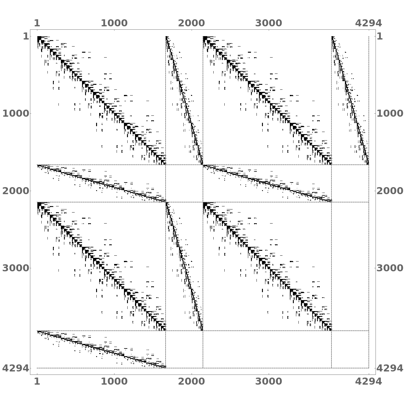
Figure 4.1: Sparsity pattern of $\boldsymbol{S}$ in (4.20) for the discrete problem of Subsec. 5.1, using $\mathcal{Q}_{4}$–$\mathcal{Q}_{3}$ Taylor-Hood elements.

4.3 Nitsche’s method for boundary conditions of Dirichlet type

In this subsection we briefly present the modifications to be made in Problem 4.2 and 4.3, respectively, for the application of Nitsche’s method to enforce Dirichlet boundary conditions; cf. Problem 3.5. In contrast to Problem 4.2 and 4.3, the Dirichlet boundary conditions are now ensured by augmenting the weak formulation with additional line integrals (surface integrals in three space dimensions); cf. Problem 3.5. In the field of computational fluid dynamics, Nitsche’s method offers appreciable advantages over the standard implementation of Dirichlet boundary condition and is particularly well suited if complex and dynamic geometries are considered. The geometry can be immersed into an underlying computational grid. The Navier-Stokes equations are then solved fulfilling the boundary conditions at the intersections between the surface discretization and the grid cells; cf. Sec. 6.

In contrast to Sec. 4.1, the continuous solution and test space is now $\boldsymbol{X}=\boldsymbol{V}\times Q$ instead of $\boldsymbol{X}_{0}=\boldsymbol{V}_{0}\times Q$. For the weak form of the time discrete Newton linearization (4.15) integration by parts then yields that

$$-\nu\bigl{<}\Delta\delta\boldsymbol{v}_{\tau}^{k+1},\boldsymbol{\psi}\bigr{>} =\nu\bigl{<}\nabla\delta\boldsymbol{v}_{\tau}^{k+1},\nabla\boldsymbol{\psi}\bigr{>}-\nu\bigl{<}\partial_{\boldsymbol{n}}\delta\boldsymbol{v}_{\tau}^{k+1},\boldsymbol{\psi}\bigr{>}_{\Gamma}\,,$$ (4.22a)

$$\bigl{<}\nabla\delta p_{\tau}^{k+1},\boldsymbol{\psi}\bigr{>} =-\bigl{<}\delta p_{\tau}^{k+1},\nabla\cdot\boldsymbol{\psi}\bigr{>}+\bigl{<}\delta p_{\tau}^{k+1}\boldsymbol{n},\boldsymbol{\psi}\bigr{>}_{\Gamma}$$ (4.22b)

where $\bigl{<}\cdot,\cdot\bigr{>}_{\Gamma}$ denotes the inner product of $L^{2}(\partial\Omega)$ and $\boldsymbol{g}_{\tau}$ is defined by means of the Hermite-type interpolation (4.9). To preserve the symmetry properties of the continuous system, the forms (cf. Problem 3.5)

$$S_{v}(\boldsymbol{\psi}) :=\nu\bigl{<}\partial_{\boldsymbol{n}}\boldsymbol{\psi},\boldsymbol{v}_{\tau}^{k}+\delta\boldsymbol{v}_{\tau}^{k+1}-\boldsymbol{g}_{\tau}\bigr{>}_{\Gamma_{D}}\,,$$ (4.23a)

$$S_{p}(\xi) :=\bigl{<}\xi\boldsymbol{n},\boldsymbol{v}_{\tau}^{k}+\delta\boldsymbol{v}_{\tau}^{k+1}-\boldsymbol{g}_{\tau}\bigr{>}_{\Gamma_{D}}$$ (4.23b)

are added on the right-hand side of (4.22a) and (4.22b), respectively, to the viscous and pressure part. Finally, we add the penalty terms (cf. Problem 3.5)

$$P_{\boldsymbol{g}_{\tau}}(\boldsymbol{\psi}):=\underbrace{\frac{\eta_{1}}{h}\nu\bigl{<}\boldsymbol{v}_{\tau}^{k}+\delta\boldsymbol{v}_{\tau}^{k+1}-\boldsymbol{g}_{\tau},\boldsymbol{\psi}\bigr{>}_{\Gamma_{D}}}_{\text{viscous penalty}}+\underbrace{\frac{\eta_{2}}{h}\bigl{<}(\boldsymbol{v}_{\tau}^{k}+\delta\boldsymbol{v}_{\tau}^{k+1}-\boldsymbol{g}_{\tau})\cdot\boldsymbol{n},\boldsymbol{\psi}\cdot\boldsymbol{n}\bigr{>}_{\Gamma_{D}}}_{\text{penalty along $\boldsymbol{n}$}}\,,$$ (4.24)

For the test space $\boldsymbol{X}=\boldsymbol{V}\times Q$, such that $(\boldsymbol{\psi},\xi)\in\boldsymbol{V}\times Q$, the integrals over the Dirichlet part $\Gamma_{D}$ of the boundary $\Gamma=\Gamma_{D}\cup\Gamma_{o}$ no longer vanish. For viscous-dominated flow, the additional terms in (4.24) enforce in weak form the boundary condition $\boldsymbol{v}-\boldsymbol{g}=\boldsymbol{0}$ on the Dirchet part of the boundary. For convection-dominated flow with a small viscosity parameter $\nu$ this enforcement is weakened in the first term on the right-hand side of (4.24). However, in the inviscid limit $\nu\rightarrow 0$, the condition $(\boldsymbol{v}-\boldsymbol{g})\cdot\boldsymbol{n}=0$ is still imposed weakly by the second of the terms on the right-hand side of (4.24) such that the normal component of the Dirichlet boundary condition is preserved in the limit case. For our computations shown in Sec. 5 we put $\eta_{1}=\eta_{2}=35$. For a more refined analysis of these parameters we refer to [38, 44]. Changing the sign of the symmetric term (4.23a) generates a non-symmetric formulation. Current results (cf. [44, 16, 17]) show that, on the one hand, this reduces the sensitivity with respect of the choice of the penalty parameters and might even allow for a parameter free penalty variant, but, on the other hand, it results in a non-symmetric structure of the underlying elliptic sub-problems, which complicates the design efficient linear solver and preconditioning techniques.

Instead of Problem 4.2 we then get following Newton iteration for the GGC¹(3) semidiscretization in time of the Navier–Stokes system (2.1) along with Nitsche’s method for enforcing Dirichlet-type boundary conditions. Due to the cumbersome derivation of the equations and the innovation of the GGC¹(3) approach all formulas are explicitly given here in order to facilitate its application and implementation and enhance the confirmability of this work.

Problem 4.4 (Newton iteration of GCC¹(3) time discretization with Nitsche’s method).

Find corrections $(\delta\boldsymbol{v}_{n,2}^{k+1},\delta\boldsymbol{v}_{n,3}^{k+1})\in\boldsymbol{V}^{2}$ and $(\delta p_{n,2}^{k+1},\delta p_{n,3}^{k+1})\in Q^{2}$ such that for all $\boldsymbol{\phi}=(\boldsymbol{\psi},\xi)\in\boldsymbol{V}^{2}\times Q^{2}$ there holds that

$$\mathcal{\widetilde{F}}_{1}(\delta\boldsymbol{v}_{n,2}^{k+1},\boldsymbol{\phi}) +\mathcal{\widetilde{F}}_{2}(\delta\boldsymbol{v}_{n,3}^{k+1},\boldsymbol{\phi})+\mathcal{\widetilde{B}}_{1}^{\,\top}(\delta p_{n,2}^{k+1},\boldsymbol{\phi})+\mathcal{\widetilde{B}}_{2}^{\,\top}(\delta p_{n,3}^{k+1},\boldsymbol{\phi})$$

$$=-\Bigl{<}\boldsymbol{q}_{1}(\boldsymbol{x}^{k})\,,\boldsymbol{\psi}\Bigr{>}+\frac{\tau_{n}\nu}{2}\Bigl{<}\partial_{\boldsymbol{n}}\delta\boldsymbol{v}_{n,2}(\boldsymbol{x}^{k})\,,\boldsymbol{\psi}\Bigr{>}_{\Gamma_{o}}-\frac{\tau_{n}\nu}{12}\Bigl{<}\partial_{\boldsymbol{n}}\delta\boldsymbol{v}_{n,3}(\boldsymbol{x}^{k})\,,\boldsymbol{\psi}\Bigr{>}_{\Gamma_{0}}$$

$$\quad+\frac{\tau_{n}\nu}{2}\Bigl{<}\partial_{\boldsymbol{n}}\boldsymbol{\psi},\boldsymbol{v}_{n,2}^{k}-\boldsymbol{g}_{n,2}\Bigr{>}_{\Gamma_{D}}-\frac{\eta_{1}\tau_{n}}{2h}\nu\Bigl{<}\boldsymbol{v}_{n,2}^{k}-\boldsymbol{g}_{n,2},\boldsymbol{\psi}\Bigr{>}_{\Gamma_{D}}$$

$$-\frac{\eta_{2}\tau_{n}}{2h}\Bigl{<}(\boldsymbol{v}_{n,2}^{k}-\boldsymbol{g}_{n,2})\cdot\boldsymbol{n},\boldsymbol{\psi}\cdot\boldsymbol{n}\Bigr{>}_{\Gamma_{D}}-\frac{\tau_{n}\nu}{12}\Bigl{<}\partial_{\boldsymbol{n}}\boldsymbol{\psi},\boldsymbol{v}_{n,3}^{k}-\boldsymbol{g}_{n,3}\Bigr{>}_{\partial\Gamma}$$

$$\quad+\frac{\eta_{1}\tau_{n}}{12h}\nu\Bigl{<}\boldsymbol{v}_{n,3}^{k}-\boldsymbol{g}_{n,3},\boldsymbol{\psi}\Bigr{>}_{\partial\Gamma_{D}}+\frac{\eta_{2}\tau_{n}}{12h}\Bigl{<}(\boldsymbol{v}_{n,3}^{k}-\boldsymbol{g}_{n,3})\cdot\boldsymbol{n},\boldsymbol{\psi}\cdot\boldsymbol{n}\Bigr{>}_{\Gamma_{D}}\,,$$

$$-\mathcal{\widetilde{B}}_{1}(\delta\boldsymbol{v}_{n,2}^{k+1},\xi) -\mathcal{\widetilde{B}}_{2}(\delta\boldsymbol{v}_{n,3}^{k+1},\xi)=-\Bigl{<}q_{2}(\boldsymbol{x}^{k})\,,\xi\Bigr{>}-\frac{\tau_{n}}{2}\Bigl{<}\xi\boldsymbol{n},\boldsymbol{v}_{n,2}^{k}-\boldsymbol{g}_{n,2}\Bigr{>}_{\Gamma_{D}}+\frac{\tau_{n}}{12}\Bigl{<}\xi\boldsymbol{n},\boldsymbol{v}_{n,3}^{k}-\boldsymbol{g}_{n,3}\Bigr{>}_{\Gamma_{D}}\,,$$

$$\mathcal{\widetilde{F}}_{3}(\delta\boldsymbol{v}_{n,2}^{k+1},\boldsymbol{\phi}) +\mathcal{F}_{4}(\delta\boldsymbol{v}_{n,3}^{k+1},\boldsymbol{\phi})+\mathcal{\widetilde{B}}_{3}^{\,\top}(\delta p_{n,3}^{k+1},\boldsymbol{\phi})=-\Bigl{<}\boldsymbol{q}_{3}(\boldsymbol{x}^{k})\,,\boldsymbol{\psi}\Bigr{>}$$

$$-\nu\Bigl{<}\partial_{\boldsymbol{n}}\delta\boldsymbol{v}_{n,2}(\boldsymbol{x}^{k})\,,\boldsymbol{\psi}\Bigr{>}_{\Gamma_{o}}+\nu\Bigl{<}\partial_{\boldsymbol{n}}\boldsymbol{\psi},\boldsymbol{v}_{n,2}^{k}-\boldsymbol{g}_{n,2}\Bigr{>}_{\Gamma_{D}}-\frac{\eta_{1}}{h}\nu\Bigl{<}\boldsymbol{v}_{n,2}^{k}-\boldsymbol{g}_{n,2},\boldsymbol{\psi}\Bigr{>}_{\Gamma_{D}}$$

$$-\frac{\eta_{2}}{h}\Bigl{<}(\boldsymbol{v}_{n,2}^{k}-\boldsymbol{g}_{n,2})\cdot\boldsymbol{n},\boldsymbol{\psi}\cdot\boldsymbol{n}\Bigr{>}_{\Gamma_{D}}\,,$$

$$-\mathcal{\widetilde{B}}_{3}(\delta\boldsymbol{v}_{n,3}^{k+1},\xi) =-\Bigl{<}q_{4}(\boldsymbol{x}^{k})\,,\xi\Bigr{>}-\Bigl{<}\xi\boldsymbol{n},\boldsymbol{v}_{n,3}^{k}-\boldsymbol{g}_{n,3}\Bigr{>}_{\Gamma_{D}}\,,$$

where the semi-linear and linear forms are defined by

$$\begin{aligned} \mathcal{\widetilde{F}}_{1}&(\delta\boldsymbol{v}_{n,2}^{k+1},\boldsymbol{\phi})\coloneqq\Bigl{<}\delta\boldsymbol{v}_{n,2}^{k+1},\boldsymbol{\psi}\Bigr{>}+\frac{\tau_{n}\nu}{2}\Bigl{<}\nabla\delta\boldsymbol{v}_{n,2}^{k+1},\nabla\boldsymbol{\psi}\Bigr{>}+\tau_{n}\Bigl{<}\nabla\delta\boldsymbol{v}_{n,2}^{k+1}\boldsymbol{a}(\boldsymbol{x}^{k}),\boldsymbol{\psi}\Bigr{>}+\tau_{n}\Bigl{<}\nabla\boldsymbol{a}(\boldsymbol{x}^{k})\delta\boldsymbol{v}_{n,2}^{k+1},\boldsymbol{\psi}\Bigr{>}\\[3.01385pt] &-\frac{\tau_{n}\nu}{2}\Bigl{<}\partial_{\boldsymbol{n}}\delta\boldsymbol{v}_{n,2}^{k+1},\boldsymbol{\psi}\Bigr{>}_{\Gamma_{D}}-\frac{\tau_{n}\nu}{2}\Bigl{<}\partial_{\boldsymbol{n}}\boldsymbol{\psi},\delta\boldsymbol{v}_{n,2}^{k+1}\Bigr{>}_{\Gamma_{D}}+\frac{\eta_{1}\tau_{n}}{2h}\nu\Bigl{<}\delta\boldsymbol{v}_{n,2}^{k+1},\boldsymbol{\psi}\Bigr{>}_{\Gamma_{D}}+\frac{\eta_{2}\tau_{n}}{2h}\Bigl{<}\delta\boldsymbol{v}_{n,2}^{k+1}\cdot\boldsymbol{n},\boldsymbol{\psi}\cdot\boldsymbol{n}\Bigr{>}_{\Gamma_{D}}\,,\end{aligned}$$

$$\begin{aligned} \mathcal{\widetilde{F}}_{2}&(\delta\boldsymbol{v}_{n,3}^{k+1},\boldsymbol{\phi})\coloneqq-\frac{\tau_{n}\nu}{12}\Bigl{<}\nabla\delta\boldsymbol{v}_{n,3}^{k+1},\nabla\boldsymbol{\psi}\Bigr{>}+\tau_{n}\Bigl{<}\nabla\delta\boldsymbol{v}_{n,3}^{k+1}\boldsymbol{b}(\boldsymbol{x}^{k}),\boldsymbol{\psi}\Bigr{>}+\tau_{n}\Bigl{<}\nabla\boldsymbol{b}(\boldsymbol{x}^{k})\delta\boldsymbol{v}_{n,3}^{k+1},\boldsymbol{\psi}\Bigr{>}\\[3.01385pt] &+\frac{\tau_{n}\nu}{12}\Bigl{<}\partial_{\boldsymbol{n}}\delta\boldsymbol{v}_{n,3}^{k+1},\boldsymbol{\psi}\Bigr{>}_{\Gamma_{D}}+\frac{\tau_{n}\nu}{12}\Bigl{<}\partial_{\boldsymbol{n}}\boldsymbol{\psi},\delta\boldsymbol{v}_{n,3}^{k+1}\Bigr{>}_{\Gamma_{D}}-\frac{\eta_{1}\tau_{n}}{12h}\nu\Bigl{<}\delta\boldsymbol{v}_{n,3}^{k+1},\boldsymbol{\psi}\Bigr{>}_{\Gamma_{D}}-\frac{\eta_{2}\tau_{n}}{12h}\Bigl{<}\delta\boldsymbol{v}_{n,3}^{k+1}\cdot\boldsymbol{n},\boldsymbol{\psi}\cdot\boldsymbol{n}\Bigr{>}_{\Gamma_{D}}\,,\end{aligned}$$

$$\begin{aligned} \mathcal{\widetilde{F}}_{3}&(\delta\boldsymbol{v}_{n,2}^{k+1},\boldsymbol{\phi})\coloneqq\nu\Bigl{<}\nabla\delta\boldsymbol{v}_{n,2}^{k+1},\nabla\boldsymbol{\psi}\Bigr{>}+\Bigl{<}\nabla\boldsymbol{v}_{n,2}^{k}\delta\boldsymbol{v}_{n,2}^{k+1},\boldsymbol{\psi}\Bigr{>}+\Bigl{<}\nabla\delta\boldsymbol{v}_{n,2}^{k+1}\boldsymbol{v}_{n,2}^{k},\boldsymbol{\psi}\Bigr{>}-\nu\Bigl{<}\partial_{\boldsymbol{n}}\delta\boldsymbol{v}_{n,3}^{k+1},\boldsymbol{\psi}\Bigr{>}_{\Gamma_{D}}\\[3.01385pt] &-\nu\Bigl{<}\partial_{\boldsymbol{n}}\boldsymbol{\psi},\delta\boldsymbol{v}_{n,2}^{k+1}\Bigr{>}_{\Gamma_{D}}+\frac{\eta_{1}}{h}\nu\Bigl{<}\delta\boldsymbol{v}_{n,2}^{k+1},\boldsymbol{\psi}\Bigr{>}_{\Gamma_{D}}+\frac{\eta_{2}}{h}\Bigl{<}\delta\boldsymbol{v}_{n,2}^{k+1}\cdot\boldsymbol{n},\boldsymbol{\psi}\cdot\boldsymbol{n}\Bigr{>}_{\Gamma_{D}}\,,\end{aligned}$$

and, with $\mathcal{B}_{i}$ as well as $\mathcal{B}_{i}^{\,\top}$, $i=1\ldots 3$, as defined in (4.17),

$$\mathcal{\widetilde{B}}_{1}(\delta\boldsymbol{v}_{n,2}^{k+1},\xi) \coloneqq\mathcal{B}_{1}+\frac{\tau_{n}}{2}\Bigl{<}\xi\boldsymbol{n},\delta\boldsymbol{v}_{n,2}^{k+1}\Bigr{>}_{\Gamma_{D}},\quad \mbox{}\mathcal{\widetilde{B}}_{1}^{\top}(\delta p_{n,2}^{k+1},\boldsymbol{\phi}) \coloneqq\mathcal{B}_{1}^{\top}-\frac{\tau_{n}}{2}\Bigl{<}\delta p_{n,2}^{k+1}\boldsymbol{n},\boldsymbol{\psi}\Bigr{>}_{\Gamma_{D}},$$

$$\mathcal{\widetilde{B}}_{2}(\delta\boldsymbol{v}_{n,2}^{k+1},\xi) \coloneqq\mathcal{B}_{2}-\frac{\tau_{n}}{12}\Bigl{<}\xi\boldsymbol{n},\delta\boldsymbol{v}_{n,3}^{k+1}\Bigr{>}_{\Gamma_{D}}, \mbox{}\mathcal{\widetilde{B}}_{2}^{\top}(\delta p_{n,3}^{k+1},\boldsymbol{\phi}) \coloneqq\mathcal{B}_{2}^{\top}+\frac{\tau_{n}}{12}\Bigl{<}\delta p_{n,3}^{k+1}\boldsymbol{n},\boldsymbol{\psi}\Bigr{>}_{\Gamma_{D}},$$

$$\mathcal{\widetilde{B}}_{3}(\delta\boldsymbol{v}_{n,2}^{k+1},\xi) \coloneqq\mathcal{B}_{3}+\Bigl{<}\xi\boldsymbol{n},\delta\boldsymbol{v}_{n,3}^{k+1}\Bigr{>}_{\Gamma}\,, \mbox{}\mathcal{\widetilde{B}}_{3}^{\,\top}(\delta p_{n,3}^{k+1},\boldsymbol{\phi}) \coloneqq\mathcal{B}_{3}^{\,\top}-\Bigl{<}\delta p_{n,3}^{k+1}\boldsymbol{n},\boldsymbol{\psi}\Bigr{>}_{\Gamma_{D}}\,.$$

The fully discrete counterpart of Problem 4.4 is obtained along the lines of Subsec. 4.2 with

$$\boldsymbol{\widetilde{F}}_{1} \coloneqq\left(\mathcal{\widetilde{F}}_{1}(\boldsymbol{\psi}_{i},\boldsymbol{\psi}_{j})\right)_{i,j=1}^{J}\,, \boldsymbol{\widetilde{F}}_{2} \coloneqq\left(\mathcal{\widetilde{F}}_{2}(\boldsymbol{\psi}_{i},\boldsymbol{\psi}_{j})\right)_{i,j=1}^{J}\,, \boldsymbol{\widetilde{F}}_{3} \coloneqq\left(\mathcal{\widetilde{F}}_{3}(\boldsymbol{\psi}_{i},\boldsymbol{\psi}_{j})\right)_{i,j=1}^{J}\,,$$ (4.26)

$$\boldsymbol{\widetilde{B}}_{1} \coloneqq\left(\mathcal{\widetilde{B}}_{1}(\boldsymbol{\psi}_{i},\boldsymbol{\psi}_{j})\right)_{i,j=1}^{J}\,, \boldsymbol{\widetilde{B}}_{2} \coloneqq\left(\mathcal{\widetilde{B}}_{2}(\boldsymbol{\psi}_{i},\boldsymbol{\psi}_{j})\right)_{i,j=1}^{J}\,, \boldsymbol{\widetilde{B}}_{3} \coloneqq\left(\mathcal{\widetilde{B}}_{3}(\boldsymbol{\psi}_{i},\boldsymbol{\psi}_{j})\right)_{i,j=1}^{J}\,,$$

$$\boldsymbol{\widetilde{B}}_{1}^{\top} \coloneqq\left(\mathcal{\widetilde{B}}_{1}^{\top}(\boldsymbol{\psi}_{i},\boldsymbol{\psi}_{j})\right)_{i,j=1}^{J}\,, \boldsymbol{\widetilde{B}}_{2}^{\top} \coloneqq\left(\mathcal{\widetilde{B}}_{2}^{\top}(\boldsymbol{\psi}_{i},\boldsymbol{\psi}_{j})\right)_{i,j=1}^{J}\,, \boldsymbol{\widetilde{B}}_{3}^{\top} \coloneqq\left(\mathcal{\widetilde{B}}_{3}^{\top}(\boldsymbol{\psi}_{i},\boldsymbol{\psi}_{j})\right)_{i,j=1}^{J}$$

replacing the corresponding quantities (4.18). The resulting block system of the Newton iteration has the same sparsity pattern as in (4.20), but is now based on the matrices (4.26).

5 Numerical experiments

In this section we study numerically the GCC¹(3) approach along with Nitsche’s method for Dirichlet boundary conditions, presented before in Sec. 4.3. Firstly, this is done by a numerical convergence study. A study of the condition number of the arising linear algebraic systems is also included. Secondly, the GCC¹(3) approach is applied to one of the popular benchmark problems proposed in [51] of flow around a cylinder. The drag and lift coefficient are computed as goal quantities of physical interest. For the sake of comparion, calculations with the standard continuous Petrov–Galerkin method of piecewise linear polynomials in time, referred to as cGP(1), are also presented. For the implementation we used the deal.II finite element library [7] along with the Trilinos library [50] for parallel computations on multiple processors.

5.1 Convergence study

For the solution $\{\boldsymbol{v},p\}$ of the Navier–Stokes system (2.1) and its fully discrete GCC¹(3) approximation $\{\boldsymbol{v}_{\tau,h},p_{\tau,h}\}$ we define the errors

$$\boldsymbol{e}^{\boldsymbol{v}}(t) \coloneqq\boldsymbol{v}(t)-\boldsymbol{v}_{\tau,h}(t)\,, e^{p}(t) \coloneqq p(t)-p_{\tau,h}(,t)\,.$$

We study the error $(\boldsymbol{e}^{\boldsymbol{v}},e^{p})$ with respect to the norms

$$\|e^{w}\|_{L^{\infty}(L^{2})} \coloneqq\max_{t\in I}\left(\int_{\Omega}\|e^{w}\|^{2}\;\mathrm{d}x\right)^{\frac{1}{2}}\,,\quad\|e^{w}\|_{L^{2}(L^{2})}\coloneqq\biggl{(}\int_{I}\int_{\Omega}\|e^{w}(t)\|^{2}\;\mathrm{d}x\,\;\mathrm{d}t\biggr{)}^{\frac{1}{2}}\,,$$

where $w\in(\boldsymbol{v},p)$. The $L^{\infty}$-norm in time is computed on the discrete time grid

$$I=\big{\{}t_{n}^{d}\mid t_{n}^{d}=t_{n-1}+d\cdot k_{n}\cdot\tau_{n},\quad k_{n}=0.001\,,\;d=0,\ldots,999\,,\;n=1,\ldots,N\big{\}}\,.$$

In our experiment we study a test setting presented in [14] and choose the right-hand side function $\boldsymbol{f}$ on $\Omega\times I=(0,1)^{2}\times(0,1]$ in such a way, that the exact solution of the Navier–Stokes system (2.1) is given by

$$\boldsymbol{v}(\boldsymbol{x},t) \coloneqq\begin{pmatrix}\cos(x_{2}\pi)\cdot\sin(t)\cdot\sin(x_{1}\pi)^{2}\cdot\sin(x_{2}\pi)\\[2.15277pt] -\cos(x_{1}\pi)\cdot\sin(t)\cdot\sin(x_{2}\pi)^{2}\cdot\sin(x_{1}\pi)\end{pmatrix}\,,$$ (5.1)

$$p(\boldsymbol{x},t) \coloneqq\cos(x_{2}\pi)\cdot\sin(t)\cdot\sin(x_{1}\pi)\cdot\cos(x_{1}\pi)\cdot\sin(x_{2}\pi)\,.$$

We prescribe a Dirichlet boundary condition (2.1c), given by the solution (5.1), on the whole boundary such that $\Gamma_{D}=\partial\Omega$, i.e. $\boldsymbol{g}=\boldsymbol{0}$. The initial condition (2.1c) is also given by (5.1), i.e. $\boldsymbol{v}_{0}=\boldsymbol{0}$. For the discretization in space the $\mathcal{Q}_{4}$–$\mathcal{Q}_{3}$ pair of the Taylor–Hood family is used; cf. Fig. 4.1. The Nitsche penalty parameters in (4.24) are fixed to $\eta_{1}=\eta_{2}=35$. We also compute the spectral condition number $\kappa_{2}(\boldsymbol{S})$ of the corresponding system matrices $\boldsymbol{S}$ of the Newton linearization, using the largest singular value $\sigma_{1}$ and its smallest one $\sigma_{n}$, by means of

$$\kappa_{2}(\boldsymbol{S})=\frac{\sigma_{1}}{\sigma_{n}}\,.$$

Table 5.1: Step sizes, resulting degrees of freedom (DoF) on each time interval $I_{n}$, spectral condition number $\kappa_{2}(\boldsymbol{S})$, errors and experimental orders of convergence (EOC) for the approximation of (5.1) with $\mathcal{Q}_{4}$–$\mathcal{Q}_{3}$ elements in space and different time integration schemes under Nitsche’s method; $\tau_{0}=$1.0$$, $h_{0}=1/\sqrt{2}$.

(a) $GCC^{1}(3)$ time integration scheme

$\tau$	$h$	$\text{DoF}_{|I_{n}}$	$\kappa_{2}(\boldsymbol{S})$	$\|e^{\;\boldsymbol{v}}\|_{L^{2}(L^{2})}$	$\|e^{\;p}\|_{L^{2}(L^{2})}$	$\|e^{\;\boldsymbol{v}}\|_{L^{\infty}(L^{2})}$	$\|e^{\;p}\|_{L^{\infty}(L^{2})}$
$\tau_{0}/2^{0}$	$h_{0}/2^{0}$	$422$	$1.0845106$	$3.09910-04$	$9.24010-04$	$7.08210-03$	$3.13910-03$
$\tau_{0}/2^{1}$	$h_{0}/2^{1}$	$1\,494$	$5.715\,73106$	$1.95410-05$	$5.51610-05$	$4.43710-05$	$1.97310-04$
$\tau_{0}/2^{2}$	$h_{0}/2^{2}$	$5\,606$	$4.369\,86107$	$1.22610-06$	$3.46810-06$	$2.78010-06$	$1.26410-05$
$\tau_{0}/2^{3}$	$h_{0}/2^{3}$	$21\,702$	$3.458\,93108$	$7.67310-08$	$2.17710-07$	$1.73410-07$	$8.01610-07$
EOC		–	–	4.00	3.99	4.00	3.98

(b) cGP(1) time integration scheme

$\tau$	$h$	$\text{DoF}_{|I_{n}}$	$\kappa_{2}(\boldsymbol{S})$	$\|e^{\;\boldsymbol{v}}\|_{L^{2}(L^{2})}$	$\|e^{\;p}\|_{L^{2}(L^{2})}$	$\|e^{\;\boldsymbol{v}}\|_{L^{\infty}(L^{2})}$	$\|e^{\;p}\|_{L^{\infty}(L^{2})}$
$\tau_{0}/2^{0}$	$h_{0}/2^{0}$	$211$	$7.213\,36104$	$1.358\,330\,274\,210-02$	$1.170\,203\,425\,810-02$	$1.789\,939\,504\,410-02$	$1.789\,939\,504\,410-02$
$\tau_{0}/2^{1}$	$h_{0}/2^{1}$	$747$	$2.237\,97105$	$3.651\,571\,487\,410-03$	$3.394\,249\,544\,210-03$	$5.662\,233\,407\,310-03$	$5.662\,233\,407\,310-03$
$\tau_{0}/2^{2}$	$h_{0}/2^{2}$	$2\,803$	$8.9551105$	$9.269\,999\,463\,210-04$	$8.277\,977\,525\,710-04$	$1.501\,781\,705\,210-03$	$1.501\,781\,705\,210-03$
$\tau_{0}/2^{3}$	$h_{0}/2^{3}$	$10\,851$	$3.587\,16106$	$2.325\,732\,192\,110-04$	$2.057\,442\,422\,410-04$	$3.805\,117\,575\,410-04$	$3.805\,117\,575\,410-04$
EOC		–	–	1.99	2.01	1.93	1.98

Table 1(a) shows the calculated errors as well as the experimental orders of convergence and the spectral condition numbers for a sequence of meshes that are successively refined in space and time. We note that a test of simultaneous convergence in space and time is thus performed. In all measured norms, we observe convergence of fourth order. This is the optimal order for the Galerkin–collocation approach GCC¹(3) with piecewise polynomials of order three in time. For the mixed approximation of the Navier–Stokes system by the $\mathcal{Q}_{4}$–$\mathcal{Q}_{3}$ pair of the Taylor–Hood family convergence of order four in space can at most be expected. Thus, the application of the Nitsche method does not deteriorate the convergence behavior. The optimal rate of convergence in time is thus obtained for the approximation of the velocity field and of the pressure variable. For comparison and to illustrate the quality of the GCC¹(3) approach, Table 1(b) also shows the results for the standard cGP$(1)$ discretization in time of second order accuracy. Of course, comparing the step sizes or number of the degrees of freedom with the errors for both approximation schemes, the higher order GCC¹(3) method is superior to the cGP(1) one. Comparing the condition of the linear algebraic systems with the computed errors for both approximation schemes, we observe that for fixed condition numbers the higher order GCC¹(3) method yields smaller errors than the cGP(1) one. Consequently, the conditioning of the linear systems, as a measure for the complexity of their iterative solution, does not suffer from the higher order combined Galerkin–collocation approximation.

Finally, we note that time-dependent boundary conditions can be captured by the Galerkin–collocation approach without loss of order of convergence. This is illustrated numerically in [5] for the wave equation.

5.2 Impact of Nitsche’s method for flow around a cylinder

In the second numerical example, we compare the effect of imposing the boundary conditions in a weak form by using Nitsche’s method (cf. Subsec. 4.3) with enforcing the boundary conditions by the definition of the underlying function space (cf. Subsec. 4.1 and 4.2) and, then, condensing the algebraic system by eliminating the degrees of freedom corresponding to the nodes on the Dirichlet part of the boundary. For the experimental setting we use the well-known DFG benchmark problem ”flow around a cylinder”, given in [51]. A section of the mesh used for the computations is shown in fig. 5.1.

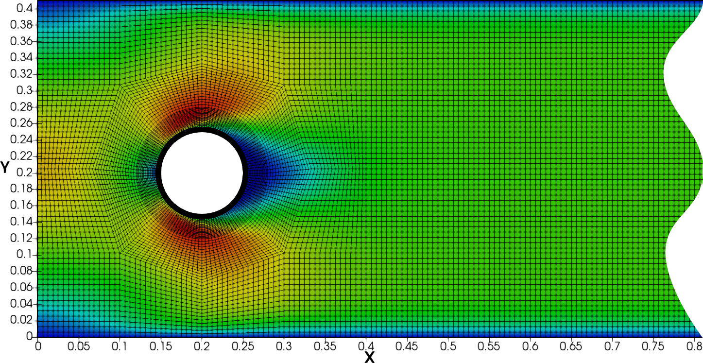
Figure 5.1: Inflow boundary at $x=0$ and part of the spatial grid around the cylinder.

We consider the time interval $I=(0,1]$, set $\nu=0.01$ and let the velocity on the inflow boundary $\Gamma_{i}$ be given by ($\boldsymbol{x}=(x,y)^{\top}$)

$$\boldsymbol{g}(x,y,t)=\begin{pmatrix}-7.13861\cdot(y-0.41)\cdot y\cdot t^{2}\\ 0\end{pmatrix}\,.$$

The maximum mean velocity of the parabolic inflow profile is reached for $T=1$ and is $\bar{U}=0.2$. With the diameter of the cylinder as the characteristic length $L=0.1$, this results in a Reynolds number $Re$ of

$$Re=\frac{\bar{U}\cdot L}{\nu}=\frac{0.2\cdot 0.1}{0.01}=2\,.$$

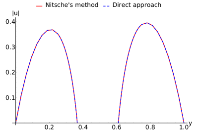
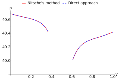
Figure 5.2: Comparison of computed velocity and pressure profiles along the $y$-axis at $x=0.2$ (cross section line through the ball’s midpoint) and $t=1$ for Nitsche’s method (weak form of Dirichlet boundary conditions) and for the enforcement of the Dirichlet boundary conditions by the definition of the function spaces with condensation of the algebraic system.

In Fig. 5.2 we compare the computed solutions along the $y$-direction at $x=0.2$ (cross section line through the ball’s midpoint) and $T=1$, that are obtained by the either methods. In the figures, the interval without having graphs is the cross section line that is covered by the ball. The computed profiles match perfectly such that no loss of accuracy is observed by the application of Nitsche’s method of enforcing Dirichlet boundary conditions for this problem of viscous flow.

5.3 GCC${}^{1}(3)$ versus cGP(1) for time-periodic flow around a cylinder

In the third numerical example we evaluate the performance properties of the Galerkin–collocation approach GCC${}^{1}(3)$ for the DFG benchmark (cf. [51]) of the time-periodic behavior of a fluid in a pipe with a circular obstacle as a more sophisticated test problem. It is set up in two space dimensions. The drag and lift coefficients of the flow on the circular cross section are computed as goal quantities of physical interest. We compare the computed results of the GCC${}^{1}(3)$ scheme with the ones obtained by the cGP(1) approximation (or Crank–Nicholson method). We use the geometrical setup as precribed in section 5.2, but consider the time interval $I=(0,10]$, set the initial time step size $\tau=0.01$, the viscosity $\nu=0.001$ and prescribe the following Dirichlet boundary condition on $\Gamma_{i}$ by

$$g(x,y,t)=\begin{pmatrix}\frac{4\cdot 1.5\cdot y(0.41-y)}{0.41^{2}}\cdot\Bigl{(}(3t^{2}-2t^{3})\cdot\bigl{(}1-\Theta(t-1)\bigr{)}+\Theta(t-1)\Bigr{)}\\[4.30554pt] 0\end{pmatrix}\,,$$ (5.2)

where $\Theta$ is the Heaviside function. Only for reasons of convenience and implementational issues, we altered the time step size slightly by choosing it as a constant, compared with the original benchmark design in [51]. Eq. (5.2) coincides with the inflow condition given in [51, p. 4], except that a smooth and non-instantaneous increase in time of the profile until $t=1$ is used. For $t\geq 1$ this results in a Reynold’s number of $Re=100$ and a time-periodic flow behaviour. With the drag and lift forces $F_{D}$ and $F_{L}$ on the circle $S$ that are defined by

$$F_{D} =\int_{S}\left(\nu\frac{\partial v_{t}}{\partial\boldsymbol{n}}n_{y}-Pn_{x}\right)\;\mathrm{d}S\,, F_{L} =-\int_{S}\left(\nu\frac{\partial v_{t}}{\partial\boldsymbol{n}}n_{x}-Pn_{y}\right)\;\mathrm{d}S\,,$$ (5.3)

where $\boldsymbol{n}$ is the normal vector on $S$ and $v_{t}$ is the tangential velocity along $\boldsymbol{t}=(n_{y},-n_{x})^{\top}$, we can compute the drag and lift coefficients $c_{D},c_{L}$ as our goal quantities by

$$c_{D} =\frac{2}{\bar{U}^{2}L}F_{D}\,, c_{L} =\frac{2}{\bar{U}^{2}L}F_{L}\,.$$ (5.4)

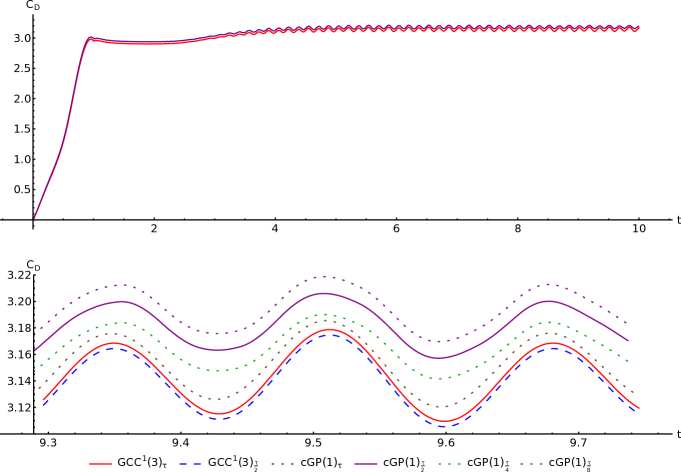
(a) Drag coefficients $C_{D}$

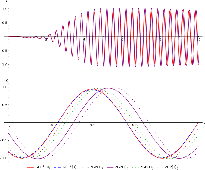
(b) Lift coefficients $c_{L}$

Figure 5.3: Computed drag and lift coefficients for the example of section 5.3 and different time discretization schemes with basic time step size $\tau$.

For the spatial discretization we use a mesh consisting of $6\,912$ cells with higher order $\mathcal{Q}_{5}$–$\mathcal{Q}_{4}$ Taylor–Hood elements. This results in $919\,104$ degrees of freedom in each time interval for the GCC${}^{1}(3)$ scheme in contrast to $459\,552$ degrees of freedom for the cGP$(1)$ method. In Fig. 5.3 we visualize the computed values for the drag and lift coefficient. The solid lines represent GCC${}^{1}(3)$ and cGP$(1)$ simulations with same number of degrees of freedom, summarized over the whole simulation time. It can be observed that the cGP$(1)$ solution converges towards the GCC${}^{1}(3)$ solution. But even with an eighth of the time step size of the GCC${}^{1}(3)$ solution it does not completely coincide with the GCC${}^{1}(3)$ solution yet. In contrast to this, the GCC${}^{1}(3)$ solution almost seems to be fully converged in the time domain with the basic time step size of $\tau$, since its further reduction to $\frac{\tau}{2}$ results in a minor change of the resulting drag and lift coefficients only. Summarizing, we can state that the GCC${}^{1}(3)$ approach is strongly superior to the cGP$(1)$ method with respect to accuracy and efficiency.

6 Outlook

We proposed and analyzed numerically higher order Galerkin–collocation time discretization schemes along with Nitsche’s method for incompressible viscous flow. The time discretization combines Galerkin approximation with the concepts of collocation. Expected optimal order convergence properties were obatined in a numerical experiment. A careful comparative numerical study with the continuous Galerin–Petrov method with piecewise linear polynomials was presented further for the DFG benchmark of flow around a cylinder with $Re=100$. The higher order Galerkin–collocation approach offered the potential of usage of much larger time steps withput loss of accuracy and, thus, improves the efficiency of the time discretization strongly. The solver of the resulting linear systems (cf. Eq. (4.20)) still continues to remain an important research topic for the future. A geometric multigrid preconditioner, based on a Vanka smoother, for GMRES outer iterations, showed promising results for the Navier–Stokes equations; cf. [28]. A similar approach was successfully used for simulations in three space dimensions of fully coupled fluid-structure interaction problems [24]. It remains to improve the current solver and develop a similar competitive solver and preconditioner for the Galerkin–collocation approach to the Navier–Stokes system. This will be a work for the future.

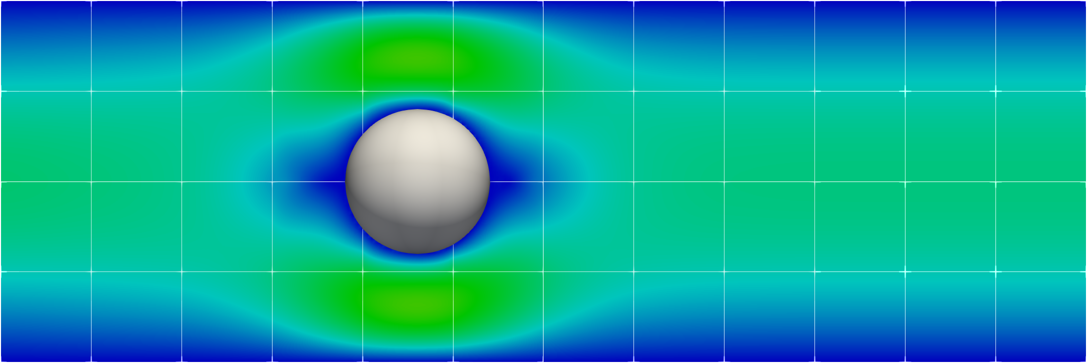
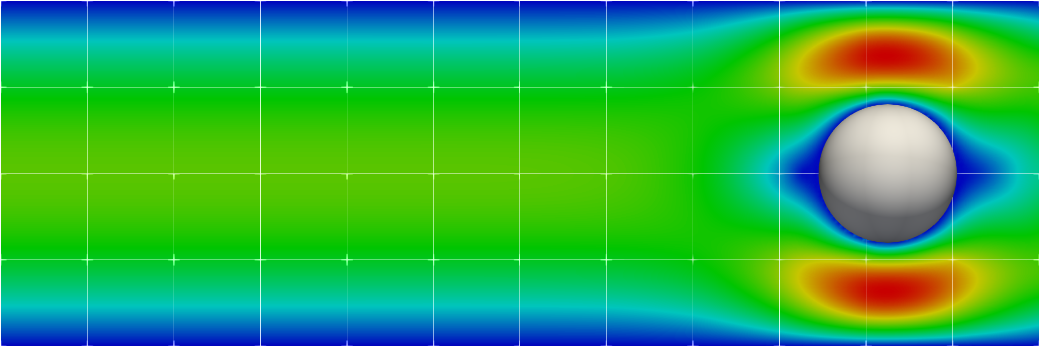
Figure 6.1: Application of Nitsche’s method with cut finite elements on a dynamic geometry.

Enforcing Dirichlet boundary conditions in a variational form by Nitsche’s method offers the potential of applying the Galerkin–collocation approach to complex flow problems in dynamic geometries with moving boundaries or interfaces. In particular, fluid structure interaction is in the scope of our interest by combining the concepts of this work with our former work [5, 6] on the numerical approximation of wave phenomena. The capability of treating dynamic domains still requires the application of the concept of fictitious domains, that is based on Nitsche’s method, together with using cut finite element techniques; cf. [20, 37, 38, 44] and the references therein. As a proof of concept, we illustrate in Fig. 6.1 a preliminary result for the simulation of flow around a moving ball. This demonstrates that the proposed Galerkin–collocation approach along with Nitsche’s method offers high potential for problems on evolving domains. In Fig. 6.1, the flow around a ball, that is moving forward and backward with prescribed velocity in a pipe, has been computed by using the Galerkin–collocation approach GCC¹(3) along with a Nitsche fictitious domain method and cut finite elements; cf. [4]. The background mesh is kept fixed for the whole simulation time such that cut elements arise, Further details will be presented in a forthcoming work since it would overburden this paper.

References

• [1] N. Ahmed, S. Becher, G. Matthies, Higher-order discontinuous Galerkin time stepping and local projection stabilization techniques for the transient Stokes problem, Comp. Meth. Appl. Mech. Eng., 313 (2017), pp. 28–52.
• [2] N. Ahmed, G. Matthies, Numerical studies of higher order variational time stepping schemes for evolutionary Navier-Stokes equations, in Z. Huang, M. Stynes, Z. Zhang (eds.), Boundary and Interior Layers, Computational and Asymptotic Methods BAIL 2016, pp. 19–34, Springer, Berlin, 2017.
• [3] G. Akrivis, C. Makridakis, R. H. Nochetto, Galerkin and Runge–Kutta methods: unified formulation, a posteriori error estimates and nodal superconvergence, Numer. Math., 118 (2011), pp. 429–456.
• [4] M. Anselmann, M. Bause, Higher order space-time approximation of the Navier–Stokes equations on dynamic domains with Nitsche’s ficititious domain method and cut elements, in progress.
• [5] M. Anselmann, M. Bause, Numerical study of Galerkin–collocation approximation in time for the wave equation, in W. Dörfler et al. (eds.), Mathematics of Wave Phenomena, Trends in Mathematics, Birkhäuser, in press, 2019, pp. 1–21; arXiv:1905.00606.
• [6] M. Anselmann, M. Bause, S. Becher, G. Matthies, Galerkin–collocation approximation in time for the wave equation and its post-processing, M2AN, DOI: 10.1051/m2an/2020033 (2020), pp. 1–25.
• [7] D. Arndt, W. Bangerth, T. Clevenger, D. Davydov, M. Fehling, D. Garcia-Sanchez, G. Harper, T. Heister, L. Heltai, M. Kronbichler, R. Maguire Kynch, M. Maier, J.-P. Pelteret, B. Turcksin, D. Wells, The deal.II Library, Version 9.1, J. Numer. Math. (2019). DOI: 10.1515/jnma-2019-0064, pp. 1–14.
• [8] M. Bause, On optimal convergence rates for higher-order Navier–Stokes approximations. I. Error estimates for the spatial discretization, IMA J. Numer. Anal., 25 (2005), pp. 812–841.
• [9] M. Bause, M. P. Bruchhäuser, U. Köcher, Flexible goal-oriented adaptivity for higher-order space-time discretization of transport problems with coupled flow, Comput. Math. Appl., submitted (2020), pp. 1–34; arXiv:2002.06855.
• [10] M. Bause, U. Köcher, F. A. Radu, F. Schieweck, Post-processed Galerkin approximation of improved order for wave equations, Math. Comp., 89 (2020), pp. 595–627.
• [11] S. Becher, G. Matthies, D. Wenzel, Variational methods for stable time discretization of first-order differential equations, in K. Georgiev, M. Todorov M, I. Georgiev (eds.), Advanced Computing in Industrial Mathematics. BGSIAM, Springer, Cham, 2018, pp. 63–75.
• [12] R. Becker, Mesh adaptation for Dirirchlet flow control via Nitsche’s method, Commun. Numer. Meth. Engrg., 18 (2002), pp. 669–680.
• [13] J. Benk, M. Ulbrich, M. Mehl, The Nitsche Method of the Navier Stokes Equations for Immersed and Moving Boundaries, in: Seventh Intern. Conf. on Comp. Fl. Dyn., 2012, pp. 1–15.
• [14] M. Besier, R. Rannacher, Goal-oriented space–time adaptivity in the finite element Galerkin method for the computation of nonstationary incompressible flow, Int. J. Numer. Meth. Fluids, 70 (9) (2012), pp. 1139–1166.
• [15] M. P. Bruchhäuser, K. Schwegler, M. Bause, Dual weighted residual based error control for nonstationary convection-dominated equations: potential or ballast?, in G. Barrenechea, J. Mackenzie, Boundary and Interior Layers, Computational and Asymptotic Methods, BAIL 2018, in press, Lecture Notes in Computational Science and Engineering 135, Springer, Cham, 2020, pp. 1–17.
• [16] T. Boiveau, E. Burman, A penalty-free Nitsche method for the weak imposition of boundary conditions in compressible and incompressible elasticity, IMA J. Numer. Anal. 36 (2) (2016), pp. 770–795.
• [17] E. Burman, A Penalty-Free Nonsymmetric Nitsche-Type Method for the Weak Imposition of Boundary Conditions, SIAM J. Numer. Anal. 50 (2012), pp. 1959–1981.
• [18] E. Burman, M. A. Fernández, Continuous interior penalty finite element method for the time-dependent Navier–Stokes equations: space discretization and convergence, Numer. Math. 107 (2007), pp. 39-77.
• [19] E. Burman, M. A. Fernández, S. Frei, A Nitsche-based formulation for fluid-structure interactions with contact, M2AN, DOI: 10.1051/m2an/2019072 (2019); pp. 1–32; arXiv:1808.08758.
• [20] E. Burmann, P. Hansbo, Fictitious domain methods using cut elements: III: A stabilized Nitsche method for Stokes system, M2AN, 48 (2014), pp. 859–874.
• [21] D. Cerroni, F. Radu, P. Zunino, Numerical solvers for a poromechanic problem with a moving boundary, Math. in Eng., 1 (4) (2019), pp. 824-848.
• [22] F. Chouly, P. Hild, A Nizsche-based method for unilateral contact problems: numerical analysis, SIAM J. Numer. Anal., 51 (2013), pp. 1295–1307.
• [23] H. C. Elman, D. J. Silvester, A. J. Wathen, Finite Elements and Fast Iterative Solvers: With Applications in Incompressible Fluid Dynamics, Oxford University Press, 2014.
• [24] L. Failer, T. Richter, A parallel Newton multigrid framework for monolithic fluid-structure interactions, 2019, pp. ; arXiv:1904.02401.
• [25] J. Heywood, R. Rannacher, Finite element approximation of the nonstationary Navier–Stokes problem. I. Regularity of solutions and second-order error estimates for spacial discretization, SIAM J. Numer. Anal. 19 (2), (1982), pp. 275-311.
• [26] S. Hussain, F. Schieweck, S. Turek, A note on accurate and efficient higher order Galerkin time stepping schemes for nonstationary Stokes equations, Open Numer. Methods, 4 (2012), pp. 35–45.
• [27] S. Hussain, F. Schieweck, S. Turek, Higher order Galerkin time discretization for nonstationary incompressible flow, in A. Cangiani et al. (eds.), Numerical Mathematics and Advanced Applications 2011, Springer, Berlin, 2013, pp. 509–517.
• [28] S. Hussain, F. Schieweck, S. Turek, Efficient Newton–multigrid solution techniques for higher order space–time Galerkin discretizations of incompressible flow, Appl. Numer. Math., 83 (2014), pp. 51–71.
• [29] V. John, A. Liakos, Time-dependent flow across a step: the slip with friction boundary condition, Int. J. Numer. Meth. Fluids, 50, (2006), pp. 713-731
• [30] V. John, Finite Element methods for Incompressible Flow Problems, Springer, Cham 2016.
• [31] C. Johnson, Discontinuous Galerkin finite element methods for second order hyperbolic problems, Comput. Methods Appl. Mech. Engrg., 107 (1993), pp. 117–129.
• [32] H. Joulak, B. Beckermann, On Gautschi’s conjecture for generalized Gauss–Radau and Gauss–Lobatto formulae, J. Comp. Appl. Math., 233 (2009), pp. 768–774.
• [33] O. Karakashian, C. Makridakis, Convergence of a continuous Galerkin method with mesh modification for nonlinear wave equations, Math. Comp., 74 (2004), pp. 85–102.
• [34] F. List, F. A. Radu, A study on iterative methods for solving Richards’ equation, Comp. Geosci., 20 (2016), pp. 341–353.
• [35] Y. Maekawa, A. Mazzucato, The Inviscid Limit and Boundary Layers for Navier–Stokes Flows, in Y. Giga, A. Novotný, Handbook of Mathematical Analysis in Mechanics of Viscous Fluids, Springer International Publishing (2018), pp. 781-828.
• [36] C. Makridakis, R. H. Nochetto, A posteriori error analysis for higher order dissipative methods for evolution problems, Numer. Math., 104 (2006), pp. 489–514.
• [37] A. Massing, M. G. Larson, A. Logg, M. Rognes, A stabilized Nitsche fictitious domain method for the Stokes problem, J. Sci. Comput., 61 (2014), pp. 604–628.
• [38] A. Massing, B. Schott, W. A. Wall, A stabilized Nitsche cut finite element method for the Oseen problem, Comput. Methods Appl. Mech. Engrg., 328 (2018), pp. 262-300.
• [39] J. Nitsche, Über ein Variationsprinzip zur Lösung von Dirichlet Problemen bei Verwendung von Teilräumen, die keinen Randbedingungen unterworfen sind (in German), Abh. Math. Sem. Univ. Hamburg, 36 (1971), pp. 9–15; DOI: 10.1007/BF02995904.
• [40] R. Pawlowski, J. Simonis, H. F. Walker, J. Shadid, Inexact Newton Dogleg Methods , SIAM J. Numer. Anal., 46(4), 2112-2132.
• [41] R. Rautmann, On optimum regularity of Navier–Stokes solutions at time $t=0$, Math. Z., 184 (1983), pp. 141–149.
• [42] H. Sohr, The Navier–Stokes Equations: An Elementary Functional Analytical Apporach, Birkhüser, Basel, (2001).
• [43] B. Schott, C. Ager, W. A. Wall, Monolithic cut finite element based approaches for fluid-structure interaction, 2018, pp. 1–41; arXiv:1807.11379.
• [44] B. Schott, Stabilized Cut Finite Element Methods for Complex Interface Coupled Flow Problems, Ph.D. Thesis, Technische Universität München, München (Mar. 2017).
• [45] F. Sonner, T. Richter, Second order pressure estimates for the Crank–Nicolson discretization of the incompressible Navier–Stokes equations, 2019, pp. 1–40; arXiv1911.03900.
• [46] O. Steinbach, Space–time finite element methods for parabolic problems, Comput. Meth. Appl. Math, 15 (2015), pp. 551–566.
• [47] O. Steinbach, H. Yang, An algebraic multigrid method for an adaptive space-time finite element discretization, Lecture Notes in Compu. Sci., 10665, Springer, Cham, 2018, pp. 63–73.
• [48] O. Steinbach, H. Yang, Space-time finite element methods for parabolic evolution equations: Discretization, a posteriori error estimation, adaptivity and solution, in (U. Langer, O. Steinbach (eds.), Space-Time Methods. Applications to Partial Differential Equations, Radon Series on Computational and Applied Mathematics, 25, de Gruyter, Berlin, 2019, pp. 207–248.
• [49] R. Temam, Navier–Stokes Equations, 3rd rev. ed., North-Holland, Amsterdam, (1984).
• [50] M. A. Heroux, J. M. Willenbring, Trilinos Users Guide, Tech. Rep. SAND2003-2952, Sandia National Laboratories (2003, updated September 2007), pp. 1–32.
• [51] S. Turek, M. Schäfer, Benchmark Computation of Laminar Flow Around a Cylinder; in Flow Simulation with High-Performance Computers II, Notes on Numerical Fluid Mechanics, 52, Vieweg, Braunschweig, 1996, pp. 547–566.
• [52] W. Varnhorn, The Stokes Equations, Akademie, Berlin, 1994.