Support Vector Machine Classifier via
Soft-Margin Loss
Abstract
Support vector machines (SVM) have drawn wide attention for the last two decades due to its extensive applications, so a vast body of work has developed optimization algorithms to solve SVM with various soft-margin losses. To distinguish all, in this paper, we aim at solving an ideal soft-margin loss SVM: soft-margin loss SVM (dubbed as -SVM). Many of the existing (non)convex soft-margin losses can be viewed as one of the surrogates of the soft-margin loss. Despite its discrete nature, we manage to establish the optimality theory for the -SVM including the existence of the optimal solutions, the relationship between them and P-stationary points. These not only enable us to deliver a rigorous definition of support vectors but also allow us to define a working set. Integrating such a working set, a fast alternating direction method of multipliers is then proposed with its limit point being a locally optimal solution to the -SVM. Finally, numerical experiments demonstrate that our proposed method outperforms some leading classification solvers from SVM communities, in terms of faster computational speed and a fewer number of support vectors. The bigger the data size is, the more evident its advantage appears.
Index Terms:
soft-margin loss, -SVM, proximal operator, minimizer and P-stationary point, support vectors, L0/1ADMM.1 Introduction
Support vector machines (SVM) were first introduced by Vapnik and Cortes [1] and then have been extensively applied into machine learning, statistic, pattern recognition and so forth. The basic idea of SVM is to find a maximum margin-type hyperplane in the input space that separates the training dataset. In the paper, we focus on the binary classification problem described as follows. Suppose we are given a training set where are the input vectors and are the output labels. The purpose of SVM is to train a hyperplane with and to be estimated by the training set. For any new input vector , one can predict its label by if and otherwise. In order to find an optimal hyperplane, there are two possible scenarios: linearly separable and inseparable training data. If the training data is linearly separated in the input space, then the unique optimal hyperplane can be obtained by solving a convex quadratic programming:
| (1) | |||||
| s.t. |
where . The above model is known as the hard-margin SVM because it requires correct classifications of all training samples. When it comes to the training data being linearly inseparable in the input space, the popular approach is to allow violations in the satisfaction of the constraints in (1) and penalize such violations in the objective function, namely,
| (2) |
where is a penalty parameter and . Here, is one of loss functions that aims at penalizing some sufficiently incorrectly classified samples and leaving the others. The above model is known as soft-margin SVM, allowing misclassified training samples. Authors in [1, 2, 3] have pointed out that the ideal soft-margin SVM is
| (3) |
where the soft-margin loss function is given by
| (4) |
and . We name (3) as -SVM, which minimizes the number of soft-margin misclassified samples. It is worth mentioning that the loss function arises in binary-valued regression, and is useful in many machine learning problems: candidates include those from perceptron learning [4], deep learning [5] and distributionally robust supervised learning [6]. However, the -SVM is NP-hard [7, 8] since the loss is nonconvex and discontinuous, and up to now, it has not been fundamentally well investigated.
As far as we know, this is the first paper that establishes the optimality theory for the -SVM and develops an effective algorithm aiming at pursuing an optimal solution to (3). The main contributions are summarized as follows.
(C1) We prove that the globally optimal solutions to the -SVM exist and also establish its optimality condition aiming at finding such solutions. The condition has a close relationship to the P-stationary point which is very practical to solve the -SVM, even though the problem is NP-hard.
(C2) Recall that the vector that maximizes the margin can be shown to have the form:
| (5) |
where is a solution to the dual problem of (1). The training vectors corresponding to non-zero are called support vectors [1], [9]. In this paper, the P-stationary point allows us to define the support vectors which coincide with the non-zero elements of the Lagrangian multiplier of (3). From the point of the optimization, the Lagrangian multiplier can be treated as a solution to the dual problem of (3), even though the dual problem is difficult to be derived due to the discreteness of . Therefore, support vectors are standard support vectors. Furthermore, we show that all support vectors fall into the support hyperplanes , where is a P-stationary point of (3). Hence, the number of support vectors are naturally expected to be no greater than the number of the standard support vectors. This is also testified by our numerical experiments.
(C3) When it comes to solving the problem (3), we adopt the famous alternating direction method of multipliers (ADMM), where one of its sub-problems is addressed by the proximal operator involved in the P-stationary point, which together with the idea of support vectors allows us to define a working set in each step. Indices of vectors out of this working set will be discarded, so the proposed method has a considerably low computational complexity and thus runs super fast. We prove that the limit point of the generated sequence is a P-stationary point and also a locally optimal solution to the problem (3). This means the final classifier only uses a small number of support vectors based on the statements in C2.
(C4) Comparing with some leading classification solvers for addressing the SVM problems on synthetic and real datasets, extensive numerical experiments demonstrate that our proposed method achieves better performance including higher prediction accuracy, a fewer number of support vectors and faster computational speed. In addition, the numerical comparison also certifies the robustness to the outliers of the -SVM.
The remainder of this paper is organized as follows. In the next section, a brief overview of various soft-margin loss functions used in (2) will be given. Section 3 establishes the optimality theory including the existence of a globally optimal solution to the problem (3) and the relationships between a P-stationary point and an optimal solution. In Section 4, we will introduce the support vectors and cast a fast ADMM whose each step is integrated by a working set strategy inspired by the support vectors. Numerical experiments and concluding remarks are given in the last two sections.
2 Related work
The discrete nature of in -SVM (3) limits its wide applications. Therefore, most previous work [10, 11] focus on the continuous surrogates of (3), namely, in (2) is a continuous approximation of . We mention two typical classes of such surrogate soft-margin loss functions [3]. The first one consists of the convex soft-margin loss functions. An impressive body of work has designed such kinds of functions since they make the corresponding SVM problems easier to deal with. Here, we only review some popular ones.
- •
-
•
Pinball soft-margin loss function: , with which is still non-differentiable at and unbounded. SVM with this soft-margin loss function was proposed in [13], [14] to pay penalty for all training samples. There is a quadratic programming solver embedded in Matlab to solve the SVM with pinball soft-margin loss function [14].
- •
- •
- •
- •
As the above loss functions are convex, their corresponding SVM models are not difficult to be dealt with [12, 13, 14, 15, 16, 17, 18, 19, 20, 21, 22, 23, 24]. However, the convexity often induces the unboundedness [25, 26], which weakens the robustness of those loss functions to outliers from the training data. To overcome such a drawback, one can set an upper bound and enforce the loss to stop increasing after a certain point. This gives rise to the second group: the nonconvex soft-margin loss functions.
- •
-
•
Truncated pinball soft-margin loss function [29] (truncated right side of pinball loss function): with and It is non-differentiable at and and unbounded. The penalty is fixed at for and is linear otherwise.
-
•
Asymmetrical truncated pinball soft-margin loss function [30] (truncated two side of pinball loss function): with and This function is non-differentiable at and but bounded. The penalty is fixed at for and at for but is linear otherwise.
-
•
Sigmoid soft-margin loss function [31]: with . It is a smooth and bounded function. It penalizes all training samples.
- •
- •
Compared to convex soft-margin loss functions, most nonconvex ones are less sensitive to feature noise or outliers due to their boundedness. Apparently, nonconvexity would lead to difficulties of computations in terms of solving the corresponding SVM models [25, 26, 28, 27, 29, 30, 31, 32, 33, 34, 35, 36, 37, 10, 11].
3 Optimality Theory of -SVM
For convenience of our subsequent analysis, denote
| (6) | |||||
where . Moreover, the zero-norm of the vector is denoted by which counts the number of its non-zero elements. It is easy to see that Then the soft-margin loss function in (4) can be rewritten as
This indicates
| (7) | |||||
Hence, the function computes the number of all positive elements in . We call it the soft-margin loss function. Borrowing these notation, the -SVM (3) is equivalent to the following optimization problem,
| (8) |
or the following problem with an extra variable ,
| s.t. |
Recall the sparse optimization problem , where is a given penalty parameter and is smooth or nonsmooth function. Due to the combinatorial nature of , the above sparse optimization problem is generally NP-hard. However, this problem has wide applications in linear and nonlinear compressive sensing, robust linear regression, deep learning, etc. Hence it has been extensively studied by a lot of researchers in different communities. More recently, by utilizing continuous optimization theory, the optimality conditions and algorithms for such a problem are successfully established by some researchers in optimization community [38, 39, 40, 41, 42, 43].
Observe the -SVM model (8) or (3). We found that it has same structure as the above sparse optimization model with difference between and . Similarly, by utilizing continuous optimization theory, we do the optimality analysis of (8) or (3) in this section.
3.1 Existence of -SVM Minimizer
Firstly, we show the existence of a global minimizer (a minimizer is often phrased as an optimal solution) to (8), a premise of the optimality condition of the -SVM.
Theorem 3.1
Given with . Then the globally optimal solution to (8) exists and the solution set is bounded.
The proof of Theorem 3.1 is given in Supplement S.1. For any , since , we have the following observations
where and are the number of positive and negative . Therefore, let be an optimal solution to (8) (such a solution exists by Theorem 3.1), then
In numerical experiments, this gives us a clue to set some starting points satisfying
| (11) |
3.2 First-Order Optimality Condition
From the perspective of optimization, establishing the optimality conditions of an optimization problem is a key step in theoretical analysis, because those conditions effectively benefits for the algorithmic design. Now turn our attention on the -SVM model (3).
Definition 3.1 (P-stationary point of (3))
For a given , we say is a proximal stationary (P-stationary) point of (3) if there is a Lagrangian multiplier and a constant such that
| (12) |
where
| (13) |
and . The above equation (13) is termed as proximal operator, whose solution has been derived in Supplement S.2.
The proximal operator is the key in the optimality analysis (see Theorem 3.2 below) and algorithmic design (see Section 4.2) of -SVM. Using the above definition, we reveal the relationship between local/global minimizer and a P-stationary point of -SVM. To proceed more, let
| (14) |
where is the generalized inverse of , and where is the maximum eigenvalue of Thus, we have following theorem.
Theorem 3.2
The following relations hold for (3).
-
(i)
A globally optimal solution is also a P-stationary point with if is full column rank.
-
(ii)
A P-stationary point with is also a locally optimal solution.
The proof of Theorem 3.2 is given in Supplement S.3. Note that being full column rank implies , i.e., the number of samples is greater than the number of features. However, from Theorem 3.2 (ii), if we find a P-stationary point of the problem (3), then it must be a locally optimal solution without any assumptions. No requirement of is enforced. Our numerical experiments testify that our proposed algorithm based on the idea of the P-stationary point works well for both cases: and .
3.3 Extension
In Section 3.2, we established the first-order optimality condition for (3), i.e., (8), which is an unconstrained optimization problem. This can be regarded as a special case of the following general optimization model
| (15) |
where is a given penalty parameter and is a smooth function and gradient Lipschitz continuous with a Lipschitz constant .
Similarly, we introduce the proximal stationary point of (15) as below.
Definition 3.2 (P-stationary point of (15))
For a given , we say is a proximal stationary (P-stationary) point of problem (15) if there is a constant such that
| (16) |
where, is the gradient of .
The following theorem reveals the relationship between a local/global minimizer and a P-stationary point of (15), whose the proof is similar to that of the Theorem 3.2 and thus is omitted.
Theorem 3.3
The above two theorems state that under condition of convexity, the P-stationary point must be a local minimizer, which means that we could use the P-stationary point as a termination rule in terms of guaranteeing the local optimality of a point generated by the algorithm proposed in next section.
4 Fast Algorithm
It is well known that the classifier is decided by support vectors, see (5). If support vectors is used to design the solving algorithm, the fewer number of support vectors is, the faster the computational speed will be since fewer samples in training data are used to train the classifier. Therefore, reducing the number of support vectors tends to be important for datasets in extremely large sizes. Motivated by this, we introduce support vectors and working set strategy based on the theory in Section 3.2 and adopt the famous alternating direction method of multipliers (ADMM) to solve the -SVM (3).
4.1 Support Vectors
Let () be a P-stationary point of problem (3). Then from Definition 3.1, there is a Lagrangian multiplier and a constant such that (12) holds. Let
| (17) |
and be its complementarity set. Let be the sub-vector of indexed on and be the cardinality of . It follows from the last equation of (12) and (13) that
which is equivalent to
| (20) |
Then in (17) turns to
| (21) |
This and (20) result in
| (22) |
Taking (22) into the first equation of (12) derives
| (23) | |||||
Remark 4.1
Regarding the expression (23), we have the following comments.
-
•
Recall (5), where is a solution to the dual problem of (1). From the optimization perspective, the Lagrangian multiplier actually is a solution to the dual problem of (3). In such a sense, indeed are standard support vectors. While we call them the support vectors since they are selected by the proximal operator.
-
•
Furthermore, the third equation in (12) implies due to by (20), which and the definition (6) of yield
(24) Interestingly, the support vectors must fall into the support hyperplanes . As far as we know, the hard-margin SVM has such a property for linearly separable datasets. For linearly inseparable datasets, most soft-margin SVM can not guarantee this property. However, (24) is ensured by the -SVM regardless of the datasets being separable or inseparable. This phenomenon manifests that the -SVM could render fewer support vectors than the other soft-margin SVM models, which is also certified by our numerical experiments.
The set in (21) gives us a clue to select support vectors, which is very practical in the following algorithmic design.
4.2 L0/1ADMM via Selection of Working Set
In this subsection, we take advantages of ADMM and working set to solve the -SVM (3). We firstly give the framework of ADMM as follows. The augmented Lagrangian function of the problem (3) is given by
where is the Lagrangian multiplier and is the penalty parameter. Given the th iteration , the framework to update each component is as follows:
| (29) |
where is the dual step-size. The proximal term is
Note that if is positive semidefinite, then the above framework is the standard semi-proximal ADMM [44]. However, authors in papers [45, 46] have also investigated ADMM with the indefinite proximal terms, namely, is indefinite. The basic principle of choosing is to guarantee the convexity of -subproblem of (29). Since is strongly convex with respect to , is flexible to be chosen as an indefinite matrix.
Now, let’s see how in (21) instructs to select the support vectors. Denote . Define a working set at the th step by
| (30) |
and . Based on which, is chosen as
| (31) |
Here, for a given set , denotes the sub-matrix containing rows of indexed on . The working set and the choice of will tremendously speed up the whole computation in each step of ADMM. More precisely, we calculate each sub-problem in (29) as follows.
(i) Updating : The -subproblem in (29) is equivalent to the following problem
where the last equation is from (13) with . This together with (13) and the working set (30) suffices to
| (32) |
Therefore, updating turns to be very simple and fast.
(ii) Updating . The -subproblem in (29) is
| (33) |
It is a convex quadratic programming problem. To solve (4.2), we only need to find a solution to the equations
| (34) | |||||
which is equivalent to find a solution to the equations
| (35) |
where . To derive (35) from (34), we used two facts that by (32) and
Therefore, the term vanishes in (35), which means the working set and the choice of discard the samples . This would fasten the computation significantly if the selected is very small. In practice, (35) can be addressed efficiently by the following rules:
(iii) Updating . The -subproblem in (29) is a convex quadratic programming
which is solved by
| (38) |
where .
(iv) Updating . We update in (29) as follows
| (39) |
where and setting follows the idea in (20), namely, the part of the Lagrangian multiplier not on the working set is removed.
Overall, updating each subproblem is summarized into Algorithm 1, which is called L0/1ADMM, an abbreviation for -SVM solved by ADMM.
4.3 Convergence and Complexity Analysis
The following theorem shows that if the sequence generated by L0/1ADMM has a limit point, then it must be a P-stationary point and also a locally optimal solution to (3).
Theorem 4.1
Suppose be the limit point of the sequence generated by L0/1ADMM. Then is a P-stationary point with and also a locally optimal solution to the problem (3).
The proof of Theorem 4.1 is given in Supplement S.4. Based on the authors’ limited knowledge, the above convergence result is difficult to improve, because our L0/1ADMM deals with -SVM directly, whose objective function involves a discrete part . As a supplement, we mention some works on ADMM and its convergence analysis: for solving nonconvex nonsmooth optimization problems, see, e.g. [48, 49, 50, 51]; for solving the nonconvex soft-margin loss SVMs, see, e.g. [52, 53].
With regard to the computational complexity in each iteration of the proposed algorithm L0/1ADMM, we have the following observations:
-
•
Updating by (30) needs the complexity .
-
•
The main term involved in computing by (32) is , taking the complexity about .
-
•
To update , we compute (36) if and (37) otherwise. For the former, the dominant computations are calculating
Their computational complexities are and with , respectively. For the latter, the dominant computations are from
with the computational complexities and with , respectively. Therefore, the complexity to update in each step is
-
•
Similarly, is the most expensive computation in (38) to derive . Again its complexity is .
-
•
Same as that of updating , achieving by (39) takes complexity.
Overall, the whole computational complexity in each step of L0/1ADMM in Algorithm 1 is
If the selected working sets have low cardinalities or is very small (i.e., ), L0/1ADMM possesses a considerably low computational complexity.
With regard to non-asymptotic analysis for finding stationary points of nonsmooth nonconvex functions, see, e.g. [54].
5 Numerical experiments
In this section, we conduct numerical experiments to show the sparsity, robustness and effectiveness of the proposed L0/1ADMM (available at https://github.com/Huajun-Wang/L01ADMM) by using MATLAB (2018b) on a laptop of 32GB of memory and Inter Core i7 2.7Ghz CPU, against nine leading solvers on synthetic data and real data.
Inspired by Theorem 3.2, the P-stationary point is taken as a stopping criteria in the experiments. In the implementation, we terminate the proposed algorithm if the point () closely satisfies the conditions in (12), i.e.,
where tol is the tolerance level and
(a) Parameters setting. In our algorithm, the parameters and control the number of support vectors (see (30)), so tuning good choices of these two parameters is crucial. Hence, the standard 10-fold cross validation is employed in training datasets to select them, where is picked from and is tuned from with . The parameters with the highest cross validation accuracy are picked out. In addition, we set , maximum iteration number and the tolerance level tol. For the starting points, set . As mentioned in Section 3.1, we choose and if it meets (11), and and (or ) otherwise.
(b) Benchmark classifiers. There is an impressive body of algorithms that have been developed to solve classification problems. However, to conduct fair comparisons, we only select nine solvers that were programmed by MATLAB. Eight of them address the SVM problem and one deals with the -regularized logistic regression problem. All their parameters are also optimized by 10-fold cross validation to maximize accuracy.
-
HSVM
SVM with the hinge soft-margin loss is implemented by LibSVM ([55], https://www.csie.ntu.edu.tw/~cjlin/libsvm/), where the parameter is selected from
-
LSVM
SVM with the square soft-margin loss [17] is implemented by LibLSSVM ([56], https://www.esat.kuleuven.be/sista/lssvmlab/), where the parameter is selected from .
-
PSVM
SVM with the pinball soft-margin loss can be tackled by the traversal algorithm ([57], https://www.esat.kuleuven.be/stadius/ADB/huang/softwarePINSVM.php), where is turned from a union of and the one in [57] and is set as from [57].
-
RSVM
SVM with the ramp soft-margin loss can be addressed by CCCP ([27], https://github.com/RampSVM/RSVM), where the core subproblem of CCCP is solved by the MATLAB built-in function quadprog, while and are selected from and .
-
SSVM
SVM with the one-sided Cauchy soft-margin loss is solved by the iteratively reweighted algorithm (IRA [3], https://www.esat.kuleuven.be/stadius/ADB/feng/softwareRSVC.php). The key subproblem of IRA is solved by the CVX, and both and are tuned from .
-
LOGI
-regularized logistic regression is addressed by employing Newton algorithm ([58], https://github.com/tminka/logreg/), where the parameter is selected from .
-
PEGA
SVM with the hinge soft-margin loss is solved by employing Pegasos algorithm ([59], https://github.com/bruincui/Pegasos), where the parameter is selected from . The mini-batch size is 1 and the maximum number of iterations is 2.
-
SVRG
SVM with the squared hinge soft-margin loss is addressed by employing SVRG algorithm ([60], https://github.com/codes-kzhan/SVRG-1/blob/master/SVM/svm_SVRG.m) with selected from . The mini-batch size is 1 and the number of “passes” is . The default epoch length is 2.
-
KATY
SVM with the squared hinge soft-margin loss is addressed by Katyusha algorithm ([61], https://github.com/codes-kzhan/SVRG-1/blob/master/SVM/svm_Katyusha.m) with all parameters selected the same as these for SVRG.
In addition, all other parameters of the above nine algorithms are set to their default values.
(c) Evaluation criteria. To evaluate classification performance, we report five evaluation criteria: the testing accuracy (ACC), the number of support vectors (NSV), the size of working set per iteration (SWS/ITER), the total number of iterations (TNI) and the CPU time (CPU). Let be the testing samples data. The testing accuracy is defined as follows
where if and otherwise, and is a solution obtained by one solver. The accuracy measures the ability of a solver to correctly predict the class labels of new input samples. The higher ACC (or the smaller NSV, SWS/ITER, TNI or CPU) is, the better performance of a solver delivers.
5.1 Comparisons with Synthetic Data
For visualization, we first consider a two-dimensional example, where the features come from Gaussian distributions [14, 57]. One can observe that L0/1ADMM performs extraordinarily in terms of delivering a considerably small number of support vectors.
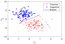
Example 5.1 (Synthetic data in without outliers)
In this example, samples with positive labels are drawn from and samples with negative labels are drawn from , where and . We generate samples with two classes having equal numbers, and then evenly split all samples into a training set and a testing set.
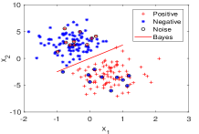
Data generated in this way has centralized features of each class. For this example, the corresponding Bayes classifier is . We display Bayes classifier and 200 training samples in Figure 1 (a), where samples are no extra noises contaminated. We then add outliers on the data generated in Example 5.1 as follows.
Example 5.2 (Synthetic data in with outliers)
Firstly, samples with two classes having equal numbers are generated as in Example 5.1. Then in each class, we randomly flip percentage of labels. For instance, in samples with positive labels , we change labels to . This means percentage of samples are flipped their labels, namely outliers are generated. Here is the flapping ratio. Finally, the samples are evenly split into a training set and a testing set. In Figure 1 (b), the training set with =10% outliers are presented.
To solve these two examples, ten solvers are applied to calculate the classifier . Since data are generated randomly, to avoid randomness, we report average results of ACC, NSV, SWS/ITER, TNI and CPU over 10 times.
(d) Synthetic data without outliers. Ten solvers are applied to solve Example 5.1 with both the training and testing sample sizes being . Average results are reported in Table I, where ”” represents that the results are not obtained if one solver takes time longer than two hour (denote ””) or the required memory is out of the capacity of our laptop (denote ””), and ”3(8)” means the number of outer iterations (the average number of inner subproblem iterations). It can be clearly seen that all algorithms achieve desirable ACC and L0/1ADMM gets slightly better ones. When it comes to NSV, the result is significant different. Obviously, LSVM, PSVM and LOGI take all samples as the support vectors, while HSVM, RSVM, SSVM, PEGA, SVRG and KATY have a small number of the support vectors. It is evidently that L0/1ADMM uses a considerably small number of the support vectors. As for SWS/ITER and TNI, LSVM, PSVM, RSVM, SSVM and LOGI take all samples as the working set, while most of them use a small TNI except for PSVM. By contrast, L0/1ADMM and others select a very small portion of samples as the working set, and L0/1ADMM uses a small TNI (no more than 50 for all cases). Because of this, L0/1ADMM consumes the shortest CPU time.
(e) Synthetic data with outliers. For Example 5.2, we fix while alter the flapping ratio from to see the robustness of each method to outliers. Average results are presented in Table II. Apparently, the more outliers, the smaller ACC for each solver. There is no big difference of ACC generated by ten solvers. Again, L0/1ADMM gets slightly better ACC, being more robust to outliers than the others. Similar observations to that in Table I can be seen for NSV, SWS/ITER and TNI. Moreover, the more outliers are added, the more examples become support vectors for HSVM, SSVM, PEGA, SVRG and KATY, and bigger values of TNI are generated by HSVM and PSVM. By contrast, L0/1ADMM makes use of fewer support vectors, SWS/ITER and TNI when more outliers are added. Not surprisingly, L0/1ADMM again runs the fastest.
| ACC (%) | ||||||||||
| HSVM | LSVM | PSVM | RSVM | SSVM | LOGI | PEGA | SVRG | KATY | ||
| 2000 | 97.05 | 97.05 | 97.00 | 97.05 | 97.05 | 97.05 | 97.03 | 97.01 | 97.05 | 97.05 |
| 4000 | 97.35 | 97.25 | 97.30 | 97.30 | 97.33 | 97.32 | 97.25 | 97.26 | 97.33 | 97.35 |
| 6000 | 97.33 | 97.28 | 97.33 | 97.24 | 97.33 | 97.22 | 97.16 | 97.33 | 97.30 | |
| 8000 | 96.96 | 96.91 | 96.89 | 96.91 | 96.96 | 96.96 | 96.93 | 96.94 | 96.96 | |
| 10000 | 97.20 | 97.18 | 97.16 | 97.19 | 97.20 | 97.18 | 97.16 | 97.18 | 97.18 | |
| NSV | ||||||||||
| 2000 | 7 | 187 | 2000 | 2000 | 96 | 146 | 2000 | 198 | 184 | 192 |
| 4000 | 10 | 301 | 4000 | 4000 | 141 | 289 | 4000 | 325 | 332 | 295 |
| 6000 | 18 | 439 | 6000 | 6000 | 201 | 6000 | 453 | 444 | 452 | |
| 8000 | 26 | 571 | 8000 | 8000 | 223 | 8000 | 566 | 579 | 563 | |
| 10000 | 22 | 658 | 10000 | 10000 | 240 | 10000 | 669 | 675 | 648 | |
| SWS/ITER | ||||||||||
| 2000 | 22 | 2 | 2000 | 2000 | 2000 | 2000 | 2000 | 1 | 1 | 1 |
| 4000 | 31 | 2 | 4000 | 4000 | 4000 | 4000 | 4000 | 1 | 1 | 1 |
| 6000 | 35 | 2 | 6000 | 6000 | 6000 | 6000 | 6000 | 1 | 1 | 1 |
| 8000 | 38 | 2 | 8000 | 8000 | 8000 | 8000 | 8000 | 1 | 1 | 1 |
| 10000 | 46 | 2 | 10000 | 10000 | 10000 | 10000 | 10000 | 1 | 1 | 1 |
| TNI | ||||||||||
| 2000 | 20 | 259 | 14 | 1216 | 3(8) | 2(13) | 8 | 4000 | 4000 | 4000 |
| 4000 | 28 | 463 | 14 | 2325 | 3(16) | 3(18) | 9 | 8000 | 8000 | 8000 |
| 6000 | 34 | 639 | 15 | 3750 | 4(15) | 9 | 12000 | 12000 | 12000 | |
| 8000 | 40 | 772 | 16 | 5247 | 4(21) | 9 | 16000 | 16000 | 16000 | |
| 10000 | 47 | 961 | 16 | 6326 | 5(23) | 10 | 20000 | 20000 | 20000 | |
| CPU (seconds) | ||||||||||
| 2000 | 0.002 | 0.014 | 0.221 | 9.642 | 3.969 | 132.5 | 0.034 | 0.028 | 0.024 | 0.025 |
| 4000 | 0.006 | 0.022 | 0.626 | 67.58 | 16.29 | 2043 | 0.112 | 0.089 | 0.087 | 0.088 |
| 6000 | 0.008 | 0.036 | 1.200 | 209.9 | 31.44 | 0.204 | 0.133 | 0.126 | 0.131 | |
| 8000 | 0.013 | 0.069 | 2.342 | 493.2 | 65.25 | 0.536 | 0.194 | 0.185 | 0.188 | |
| 10000 | 0.018 | 0.094 | 3.951 | 775.3 | 124.7 | 0.938 | 0.281 | 0.266 | 0.268 | |
| ACC (%) | ||||||||||
| HSVM | LSVM | PSVM | RSVM | SSVM | LOGI | PEGA | SVRG | KATY | ||
| 0.00 | 97.16 | 97.08 | 97.10 | 97.16 | 97.16 | 97.12 | 97.08 | 97.03 | 97.16 | 97.16 |
| 0.05 | 92.65 | 92.46 | 92.50 | 92.60 | 92.65 | 92.57 | 92.58 | 92.54 | 92.30 | 92.35 |
| 0.10 | 87.98 | 87.78 | 87.78 | 87.90 | 87.90 | 87.90 | 87.70 | 87.68 | 87.46 | 87.45 |
| 0.15 | 83.06 | 82.86 | 82.80 | 82.98 | 83.06 | 83.04 | 82.93 | 82.98 | 82.88 | 82.88 |
| 0.20 | 78.30 | 78.16 | 78.12 | 78.28 | 78.28 | 78.20 | 78.16 | 78.21 | 78.17 | 78.18 |
| NSV | ||||||||||
| 0.00 | 21 | 364 | 5000 | 5000 | 184 | 329 | 5000 | 372 | 359 | 357 |
| 0.05 | 20 | 947 | 5000 | 5000 | 175 | 874 | 5000 | 942 | 953 | 945 |
| 0.10 | 17 | 1385 | 5000 | 5000 | 170 | 1015 | 5000 | 1365 | 1373 | 1389 |
| 0.15 | 16 | 1795 | 5000 | 5000 | 161 | 1657 | 5000 | 1790 | 1781 | 1792 |
| 0.20 | 13 | 2160 | 5000 | 5000 | 137 | 1989 | 5000 | 2177 | 2175 | 2187 |
| SWS/ITER | ||||||||||
| 0.00 | 34 | 2 | 5000 | 5000 | 5000 | 5000 | 5000 | 1 | 1 | 1 |
| 0.05 | 31 | 2 | 5000 | 5000 | 5000 | 5000 | 5000 | 1 | 1 | 1 |
| 0.10 | 30 | 2 | 5000 | 5000 | 5000 | 5000 | 5000 | 1 | 1 | 1 |
| 0.15 | 28 | 2 | 5000 | 5000 | 5000 | 5000 | 5000 | 1 | 1 | 1 |
| 0.20 | 27 | 2 | 5000 | 5000 | 5000 | 5000 | 5000 | 1 | 1 | 1 |
| TNI | ||||||||||
| 0.00 | 32 | 584 | 15 | 3042 | 3(25) | 3(21) | 9 | 10000 | 10000 | 10000 |
| 0.05 | 30 | 3726 | 15 | 3126 | 4(18) | 3(21) | 9 | 10000 | 10000 | 10000 |
| 0.10 | 29 | 5128 | 15 | 3268 | 4(17) | 3(21) | 9 | 10000 | 10000 | 10000 |
| 0.15 | 26 | 8423 | 15 | 3373 | 5(13) | 3(21) | 9 | 10000 | 10000 | 10000 |
| 0.20 | 25 | 10776 | 15 | 3443 | 5(13) | 3(21) | 9 | 10000 | 10000 | 10000 |
| CPU (seconds) | ||||||||||
| 0.00 | 0.008 | 0.027 | 0.801 | 93.11 | 22.53 | 4047 | 0.149 | 0.117 | 0.108 | 0.112 |
| 0.05 | 0.008 | 0.075 | 0.823 | 101.3 | 20.99 | 4069 | 0.131 | 0.119 | 0.114 | 0.115 |
| 0.10 | 0.006 | 0.123 | 0.853 | 105.4 | 19.43 | 4084 | 0.147 | 0.118 | 0.111 | 0.112 |
| 0.15 | 0.005 | 0.172 | 0.885 | 108.3 | 18.96 | 4092 | 0.152 | 0.118 | 0.110 | 0.111 |
| 0.20 | 0.005 | 0.236 | 0.898 | 110.6 | 18.41 | 4094 | 0.165 | 0.119 | 0.115 | 0.116 |
5.2 Comparisons with Real Data
We now apply these solvers to deal with 14 real datasets. Their information are presented in Table III, where the last six datasets have the testing data.
Example 5.3 (Real data without outliers)
We perform 10-fold cross validation for the first eight datasets. Each one is randomly split into ten parts, with one part being used for testing and the rest being used for training. We then record average results to evaluate performance. In our experiments, all features are scaled to .
| Training data | Testing data | Features | |
| Datasets | |||
| Colon-cancer (col) | 62 | 0 | 2000 |
| Australian (aus) | 690 | 0 | 14 |
| Two-norm (two) | 7400 | 0 | 20 |
| Mushrooms (mus) | 8124 | 0 | 112 |
| Adult (adu) | 17887 | 0 | 13 |
| Covtype.binaty (cov) | 581012 | 0 | 54 |
| SUSY (sus) | 5000000 | 0 | 18 |
| HIGGS (hig) | 11000000 | 0 | 28 |
| Lekemia (lek) | 38 | 34 | 7129 |
| Splice (spl) | 1000 | 2175 | 60 |
| A6a (a6a) | 11220 | 21341 | 123 |
| W6a (w6a) | 17188 | 32561 | 300 |
| W8a (w8a) | 49749 | 14951 | 300 |
| ijcnn1 (ijc) | 49990 | 91701 | 22 |
| ACC (%) | ||||||||||
| Data | HSVM | LSVM | PSVM | RSVM | SSVM | LOGI | PEGA | SVRG | KATY | |
| col | 90.23 | 64.52 | 85.48 | 77.69 | 89.68 | 85.87 | 86.74 | 89.68 | 89.68 | 89.68 |
| aus | 86.23 | 85.51 | 85.80 | 85.80 | 86.02 | 85.98 | 86.18 | 86.04 | 86.18 | 86.23 |
| lek | 82.35 | 58.82 | 79.41 | 58.82 | 76.47 | 82.35 | 82.35 | 82.35 | 82.35 | 82.35 |
| spl | 85.52 | 88.97 | 85.75 | 85.52 | 85.47 | 85.47 | 85.15 | 84.18 | 85.44 | 85.33 |
| two | 98.37 | 98.02 | 97.97 | 97.97 | 98.24 | 97.78 | 98.10 | 98.37 | 98.24 | |
| mus | 100.0 | 100.0 | 100.0 | 100.0 | 100.0 | 100.0 | 100.0 | 100.0 | 100.0 | |
| adu | 83.90 | 83.29 | 83.01 | 83.07 | 83.79 | 82.95 | 83.29 | 83.34 | 83.90 | |
| a6a | 84.90 | 84.18 | 84.55 | 84.69 | 84.72 | 84.76 | 84.36 | 84.72 | 84.78 | |
| w6a | 97.93 | 97.21 | 97.58 | 97.21 | 97.86 | 95.13 | 97.24 | 97.61 | 97.57 | |
| w8a | 98.54 | 98.27 | 97.43 | 97.57 | 97.59 | |||||
| ijc | 94.33 | 92.73 | 93.49 | 93.35 | 93.56 | |||||
| cov | 71.79 | 68.93 | 69.83 | 69.77 | ||||||
| sus | 67.58 | 64.28 | 65.62 | 65.86 | ||||||
| hig | 65.21 | 58.12 | 59.13 | 59.46 | ||||||
| NSV | ||||||||||
| col | 34 | 46 | 54 | 54 | 38 | 40 | 54 | 46 | 45 | 46 |
| aus | 24 | 203 | 621 | 621 | 89 | 177 | 621 | 198 | 195 | 202 |
| lek | 26 | 31 | 38 | 38 | 29 | 31 | 38 | 33 | 34 | 31 |
| spl | 70 | 607 | 1000 | 1000 | 87 | 332 | 1000 | 632 | 615 | 612 |
| two | 30 | 758 | 6600 | 6600 | 108 | 6600 | 783 | 775 | 788 | |
| mus | 135 | 550 | 7311 | 7311 | 506 | 7311 | 578 | 575 | 568 | |
| adu | 113 | 6379 | 16098 | 16098 | 1247 | 16098 | 6407 | 6386 | 6394 | |
| a6a | 370 | 4346 | 11220 | 11220 | 1247 | 11220 | 4562 | 4575 | 4582 | |
| w6a | 429 | 1128 | 17188 | 17188 | 946 | 17188 | 1146 | 1152 | 1138 | |
| w8a | 867 | 2857 | 2582 | 2579 | 2561 | |||||
| ijc | 215 | 8508 | 8535 | 8612 | 8608 | |||||
| cov | 137 | 3e5 | 3e5 | 3e5 | ||||||
| sus | 730 | 2e6 | 2e6 | 2e6 | ||||||
| hig | 1338 | 5e6 | 5e6 | 5e6 | ||||||
| SWS/ITER | ||||||||||
| col | 37 | 2 | 54 | 54 | 54 | 54 | 54 | 1 | 1 | 1 |
| aus | 66 | 2 | 621 | 621 | 621 | 621 | 621 | 1 | 1 | 1 |
| lek | 29 | 2 | 38 | 38 | 38 | 38 | 38 | 1 | 1 | 1 |
| spl | 94 | 2 | 1000 | 1000 | 1000 | 1000 | 1000 | 1 | 1 | 1 |
| two | 136 | 2 | 6600 | 6600 | 6600 | 6600 | 1 | 1 | 1 | |
| mus | 772 | 2 | 7311 | 7311 | 7311 | 7311 | 1 | 1 | 1 | |
| adu | 1105 | 2 | 16098 | 16098 | 16098 | 16098 | 1 | 1 | 1 | |
| a6a | 569 | 2 | 11220 | 11220 | 11220 | 11220 | 1 | 1 | 1 | |
| w6a | 656 | 2 | 17188 | 17188 | 17188 | 17188 | 1 | 1 | 1 | |
| w8a | 1284 | 2 | 1 | 1 | 1 | |||||
| ijc | 829 | 2 | 1 | 1 | 1 | |||||
| cov | 1520 | 1 | 1 | 1 | ||||||
| sus | 2814 | 1 | 1 | 1 | ||||||
| hig | 3225 | 1 | 1 | 1 | ||||||
| TNI | ||||||||||
| col | 30 | 41 | 2 | 31 | 2(2) | 2(4) | 4 | 108 | 108 | 108 |
| aus | 25 | 423 | 17 | 869 | 2(7) | 3(26) | 6 | 1242 | 1242 | 1242 |
| lek | 18 | 89 | 2 | 42 | 2(2) | 3(17) | 25 | 76 | 76 | 76 |
| spl | 63 | 595 | 28 | 1276 | 2(9) | 4(28) | 9 | 2000 | 2000 | 2000 |
| two | 50 | 660 | 75 | 3417 | 4(11) | 12 | 13200 | 13200 | 13200 | |
| mus | 21 | 1623 | 106 | 3685 | 4(12) | 18 | 14622 | 14622 | 14622 | |
| adu | 26 | 4766 | 157 | 7720 | 5(21) | 15 | 32196 | 32196 | 32196 | |
| a6a | 183 | 3032 | 289 | 6873 | 5(27) | 16 | 22440 | 22440 | 22440 | |
| w6a | 121 | 1450 | 404 | 14417 | 7(32) | 28 | 34376 | 34376 | 34376 | |
| w8a | 195 | 8124 | 99498 | 99498 | 99498 | |||||
| ijc | 146 | 6681 | 99980 | 99980 | 99980 | |||||
| cov | 103 | 1.05 | 1.05 | 1.05 | ||||||
| sus | 117 | 9.0 | 9.0 | 9.0 | ||||||
| hig | 124 | 1.98 | 1.98 | 1.98 | ||||||
| CPU (seconds) | ||||||||||
| col | 0.021 | 0.009 | 0.001 | 0.010 | 0.003 | 1.488 | 0.182 | 0.015 | 0.012 | 0.014 |
| aus | 0.005 | 0.014 | 0.033 | 0.874 | 0.650 | 87.23 | 0.021 | 0.004 | 0.004 | 0.004 |
| lek | 0.072 | 0.057 | 0.004 | 0.010 | 0.008 | 54.36 | 36.10 | 0.029 | 0.024 | 0.026 |
| spl | 0.043 | 0.117 | 0.083 | 7.976 | 0.631 | 384.2 | 0.151 | 0.036 | 0.032 | 0.033 |
| two | 0.054 | 0.265 | 2.506 | 516.7 | 139.2 | 1.591 | 0.171 | 0.164 | 0.166 | |
| mus | 0.074 | 0.997 | 3.419 | 769.5 | 153.4 | 6.942 | 0.422 | 0.412 | 0.416 | |
| adu | 0.576 | 3.775 | 24.58 | 1633.4 | 1013.2 | 5.032 | 0.775 | 0.732 | 0.744 | |
| a6a | 0.172 | 4.405 | 40.64 | 1472.5 | 1037.3 | 6.046 | 1.083 | 1.025 | 1.031 | |
| w6a | 0.226 | 1.532 | 170.9 | 5947.2 | 2747.4 | 41.21 | 1.314 | 1.186 | 1.232 | |
| w8a | 2.576 | 64.33 | 4.863 | 4.227 | 4.316 | |||||
| ijc | 0.573 | 36.95 | 1.526 | 1.247 | 1.316 | |||||
| cov | 3.870 | 14.37 | 13.88 | 13.91 | ||||||
| sus | 10.38 | 137.6 | 132.4 | 133.7 | ||||||
| hig | 14.26 | 281.3 | 269.5 | 270.1 | ||||||
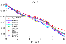
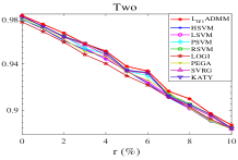
Example 5.4 (Real data with outliers)
To see the influence of the real data with outliers, we select six datasets from small sizes to moderate sizes in Table III. They are col, aus, two, mus, adu and a6a. Same processes as in Example 5.3 are then applied into the first five datasets. Finally, percentage of training and testing samples are randomly treated as outliers (i.e., their labels are flipped).
(f) Real data without outliers. The average results are recorded in Table IV, where “” represents the number greater than . It can be clearly seen that L0/1ADMM outperforms the others in terms of the highest ACC, smallest NSV and shortest CPU for most datasets, and uses a small SWS/ITER and TNI. For instance, L0/1ADMM predicts more than 90% samples correctly for col whilst HSVM and PSVM only get less than 80% correct predictions. Compared with those generated by the other nine solvers, NSV from L0/1ADMM is relatively small. As for SWS/ITER, L0/1ADMM takes a small samples as the working set, which testifies that our constructed working set strategy is very effective to reduce the cost of per iteration. As for TNI, L0/1ADMM uses a few TNI compared with PSVM, PEGA, SVRG and KATY. For the computational speed, PEGA, SVRG and KATY present the advantage of CPU for dealing with small scale datasets. The L0/1ADMM runs super fast for datasets in big sizes, 0.573 seconds v.s. 36.95 seconds by HSVM for data ijc. In addition, it only needs 14.26 seconds for the dataset hig with more than ten million samples. Overall, it seems that the bigger is, the more evident the advantage of L0/1ADMM becomes.
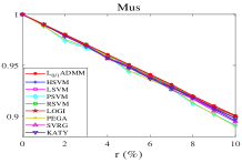
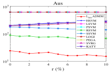
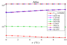
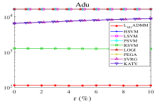
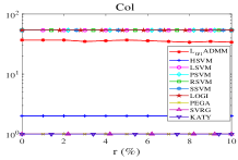
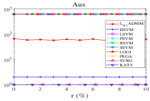
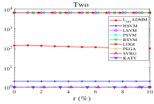
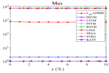
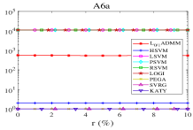
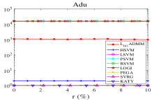
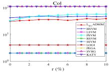
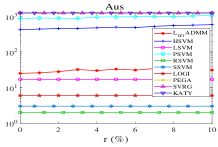
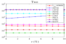
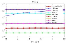
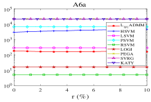
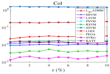
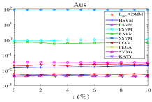
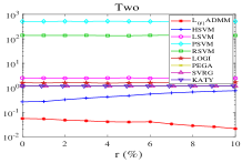
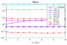
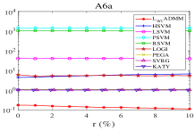
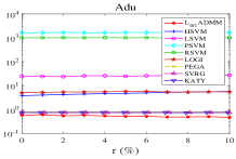
(g) Real data with outliers. Finally, we would like to see the robustness of each solver to the outliers for real datasets in Example 5.4. Again we alter the flapping ratio from . It is shown in Table IV that SSVM takes too long time for datasets: two, mus, adu and a6a. Therefore, its results related to these datasets are omitted. All lines of ACC shown in Figure 2 decline with ascending, and L0/1ADMM achieves the highest ACC. As for NSV in Figure 3, LSVM, PSVM and LOGI always treat all samples as support vectors. HSVM, SSVM, PEGA, SVRG and KATY increase NSV with the rising of . Lines from L0/1ADMM and RSVM either decline or stabilize at a level with the rising of , which means they are quite robust to , namely robust to the outliers. What is more, L0/1ADMM always renders the fewest NSV. As for SWS/ITER in Figure 4, with the rising of , L0/1ADMM stabilizes at a level for all datasets. As for TNI in Figure 5, all algorithms no big difference with the ascending of except for HSVM. For the computational speed, as demonstrated in Figure 6, L0/1ADMM outperforms the others for all datasets except for col and aus which have a very small size.
6 conclusion
In this paper, we have explored an ideal soft-margin SVM model: -SVM, which well captures the nature of the binary classification and guarantees a fewer number of support vectors than the other soft-margin SVM models. Despite the discreteness of the -SVM, the establishment of the optimality theory, associated with the P-stationary point, makes it tractable numerically. Based on the idea of support vectors inspired by the P-stationary point, a working set was cast and integrated into the proximal ADMM, which tremendously speeds up the whole computation and reduces the number of support vectors. Consequently, the proposed method performed exceptionally well with fewer support vectors and faster computational speed, especially for datasets on large scales.
Acknowledgements
The authors would like to thank the associate editor and three anonymous referees for their constructive comments, which have significantly improved the quality of the paper. This work is supported by the National Natural Science Foundation of China (11971052, 11926348-9, 61866010, 11871183), and the Natural Science Foundation of Hainan Province (120RC449).


References
- [1] C. Cortes and V. Vapnik, ”Support vector networks”, Mach. Learn., vol. 20, no. 3, pp. 273-297, 1995.
- [2] J. P. Brooks, ”Support vector machines with the ramp loss and the hard margin loss”, Oper. Res., vol. 59, no. 2, pp. 467-479, 2011.
- [3] Y. L. Feng, Y. N. Yang, X. L. Huang, S. Mehrkanoon, and J. A. K. Suykens, ”Robust support vector machines for classification with nonconvex and smooth losses”, Neural Comput., vol. 28, no. 6, pp. 1217-1247, 2016.
- [4] L. Li and H. T. Lin, ”Optimizing 0/1 loss for perceptrons by random coordinate descent”, in Proc. IEEE Int. Joint Conf. Neural Netw., 2007, pp. 649-654.
- [5] I. Goodfellow, B. Yoshua, and C. Aaron, ”Deep learning”, MIT press, 2016.
- [6] W. H. Hu, G. Niu, I. Sato, and M. Sugiyama, ”Does distributionally robust supervised learning give robust classifiers?”, in Proc. 35th Int. Conf. Mach. Learn., pp. 2029-2037, 2018.
- [7] B. K. Natarajan,” Sparse approximate solutions to linear systems”, SIAM J. Comput., vol. 24, no. 2, pp. 227-234, 1995.
- [8] E. Amaldi and V. Kann, ”On the approximability of minimizing nonzero variables or unsatisfied relations in linear systems”, Theor. Comput. Sci., vol. 209, no. 1, pp. 237-260, 1998.
- [9] A. Cotter, S. Shalev-Shwartz, and N. Srebro, ”Learning optimally sparse support vector machines”, in Proc. Int. Conf. Mach. Learn., 2013, pp. 266-274.
- [10] H. Masnadi-Shirazi and N. Vasconcelos, ”On the design of loss functions for classification: theory, robustness to outliers, and savageboost”, in Proc. Int. Conf. Neural Inf. Process. Syst., pp. 1049-1056, 2009.
- [11] Y. M. Lyu and W. I. Tsang, ”Curriculum loss: robust learning and generalization against label corruption”, arXiv preprint arXiv:1905.10045, 2019.
- [12] B. Schoelkopf and A. J. Smola,” Learning with kernels”, MIT Press, 2002.
- [13] V. Jumutc, X. Huang, and J. A. K. Suykens, ”Fixed-size pegasos for hinge and pinball loss SVM”, in Proc. IEEE Int. Joint Conf. Neural Netw.,pp. 1-7, 2013.
- [14] X. Huang, L. Shi, and J. A. K. Suykens, ”Support vector machine classifier with pinball loss”, IEEE Trans. Pattern Anal. Mach. Intell., vol. 36, no. 5, pp. 984-997, 2014.
- [15] L. Wang, J. Zhu, and H. Zou, ”Hybrid huberized support vector machines for microarray classification”, Bioinformatics, vol. 24, no. 3, pp. 412-419, 2008.
- [16] Y. Xu, I. Akrotirianakis, and A. Chakraborty, ”Proximal gradient method for huberized support vector machine”, Pattern Anal. Appl., vol. 19, no. 4, pp. 989-1005, 2016.
- [17] J. A. K. Suykens and J. Vandewalle, ”Least squares support vector machine classifiers”, Neural Process. Lett., vol. 9, no. 3, pp. 293-300, 1999.
- [18] X. Yang, L. Tan, and L. F. He, ”A robust least squares support vector machine for regression and classification with noise”, Neurocomputing, vol. 140, pp. 41-52, 2014.
- [19] T. Zhang and F. J. Oles, ”Text categorization based on regularized linear classification methods”, Information Retrieval, vol. 4, no. 1, pp. 5-31, 2008.
- [20] J. Friedman, T. Hastie, and R. Tibshirani, ”Additive logistic regression: a statistical view of boosting”, Ann. Stat., vol. 28, no. 2, pp. 337-374, 2000.
- [21] P. L. Bartlett and H. W. Marten, ”Classification with a reject option using a hinge loss”, J. Mach. Learn. Res. vol. 9, no. 8, pp. 1823-1840, 2008.
- [22] P. L. Bartlett, M. I. Jordan, and J. D. Mcauliffe, ”Large margin classifiers: convex loss, low noise, and convergence rates”, in Proc. Int. Conf. Neural Inf. Process. Syst., pp. 1173-1180, 2004.
- [23] P. L. Bartlett, M. I. Jordan, and J. D. Mcauliffe, ”Convexity, classification, and risk bounds”, J. Am. Stat. Assoc., vol. 101, no. 473, pp. 138-156, 2006.
- [24] J. H. Friedman, ”On bias, variance, 0/1-loss, and the curse-of-dimensionality”, Data Min. Knowl. Discov., vol. 1, no. 1, pp. 55-77, 1997.
- [25] L. Mason, P. L. Bartlett, and J. Baxter, ”Improved generalization through explicit optimization of margins,” Mach. Learn., vol. 38, no. 3, pp. 243-255, 2000.
- [26] F. Perez-Cruz, A. Navia-Vazquez, A. R. Figueiras-Vidal, and A. Artes-Rodriguez, ”Empirical risk minimization for support vector classifiers”, IEEE Trans. Neural Netw., vol. 14, no. 2, pp. 296-303, 2003.
- [27] R. Collobert, F. Sinz, J. Weston, L. Bottou, ”Trading convexity for scalability”, in Proc. 23th Int. Conf. Mach. Learn., 2006, pp. 201-208.
- [28] X. Huang, L. Shi, and J. A. K. Suykens, ”Ramp loss linear programming support vector machine”, J. Mach. Learn. Res., vol. 15, no. 1, pp. 2185-2211, 2014.
- [29] X. Shen, L. F. Niu, Z. Qi, and Y. J. Tian, ”Support vector machine classifier with truncated pinball loss”, Pattern Recognit., vol. 68, pp. 199-210, 2017.
- [30] L. M. Yang and H. G. Dong, ”Support vector machine with truncated pinball loss and its application in pattern recognition”, Chemometrics Intell. Lab. Syst., vol. 177, pp. 89-99, 2018.
- [31] F. Perez-Cruz, A. Navia-Vazquez, P. L. Alarcon-Diana, and A. Artes-Rodriguez, ”Support vector classifier with hyperbolic tangent penalty function”, in Proc. IEEE Int. Conf. Acoust. Speech Signal Process., pp. 3458-3461, 2000.
- [32] L. Wang, H. D. Jia, and J. Li, ”Training robust support vector machine with smooth ramp loss in the primal space”, Neurocomputing, vol. 71, no. 13, pp. 3020-2025, 2008.
- [33] I. Steinwart and A. Christmann, ”Support vector machines”, New York: Springer, 2008.
- [34] S. Y. Park and Y. F. Liu, ”Robust penalized logistic regression with truncated loss functions”, Canadian Journal of Statistics, vol. 39, no. 2, pp. 300-323, 2011.
- [35] D. L. Liu, Y. Shi, Y. J. Tian, and X. K. Huang, ”Ramp loss least squares support vector machine”, J. Comput. Sci., vol. 14, pp. 61-68, 2016.
- [36] I. Steinwart and N. Christianini, ”Sparseness of support vector machines”, J. Mach. Learn. Res., vol. 4, no. 6, pp. 1071-1105, 2004.
- [37] S. Ertekin, L. Bottou, and C. L. Giles, ”Nonconvex online support vector machines”, IEEE Trans. Pattern Anal. Mach. Intell., vol. 32, no. 4, pp. 368-381, 2010.
- [38] T. Blumensath and M. E. Davies, ”Iterative thresholding for sparse approximations”, J. Fourier Anal.Appli., vol. 14, no. 5-6, pp. 629-654, 2008.
- [39] T. Blumensath and M. E. Davies, ”Iterative hard thresholding for compressed sensing”, Appl. Comput. Harmonic Anal., vol. 27, no. 3, pp. 265-274, 2009.
- [40] Z. Lu and Y. Zhang, ”Sparse approximation via penalty decomposition methods”, SIAM J. Optim., vol. 23, no. 4, pp. 2448-2478, 2013.
- [41] Z. S. Lu, ”Iterative reweighted minimization methods for -regularized unconstrained nonlinear programming”, Math. Program., vol. 147, no.1-2, pp. 277-307, 2014.
- [42] A. Beck and N. Hallak, ”Proximal mapping for symmetric penalty and sparsity”, SIAM J. Optim., vol. 28, no. 1, pp. 496-527, 2018.
- [43] H. Zhang, L. L. Pan, and N. H. Xiu, ”Optimality conditions for locally Lipschitz optimization with -regularization”, Optim. Lett., DOI: 10.1007/s11590-020-01579-y, 2020.
- [44] M. Fazel, T. K. Pong, D. F. Sun, and P. Tseng, ”Hankel matrix rank minimization with applications to system identification and realization”, SIAM J. Matrix Anal. Appl., vol. 34, no. 3, pp. 946-977, 2013.
- [45] M. Li, D. F. Sun, and K. C. Toh, ”A majorized ADMM with indefinite proximal terms for linearly constrained convex composite optimization”, SIAM J. Optim., vol. 26, no. 2, pp. 922-950, 2016.
- [46] X. Chang, S. Liu, P. Zhao, and D. Song, ”A generalization of linearized alternating direction method of multipliers for solving two-block separable convex programming”, J. Comput. Appl. Math., vol. 357, no. 2, pp. 251-272, 2019.
- [47] G. Golub and C. F. Van-Loan, ”Matrix computations”, Johns Hopkins University Press, 1996.
- [48] Y. Wang, W. T. Yin, and J. S. Zeng, ”Global convergence of ADMM in nonconvex nonsmooth optimization”, J. Sci. Comput., vol. 78, no. 1, pp. 29-63, 2019.
- [49] G. Y. Li and T. K. Pong, ”Global convergence of splitting methods for nonconvex composite optimization”, SIAM J. Optim., vol. 25, no. 4, pp. 2434-2460, 2015.
- [50] M. Hong, Z. Luo, and M. Razaviyayn, ”Convergence analysis of alternating direction method of multipliers for a family of nonconvex problems”, SIAM J. Optim., vol. 26, no. 1, pp. 337-364, 2016.
- [51] R. I. Bot and D. K. Nguyen, ”The proximal alternating direction method of multipliers in the nonconvex setting: convergence analysis and rates”, Math. Oper. Res., vol. 45, no. 2, pp. 682-712, 2020.
- [52] F. P. Nie, Y. Z. Huang, X. Q. Wang, and H. Huang, ”New primal SVM solver with linear computational cost for big data classifications”, in Proc. 31th Int. Conf. Mach. Learn., pp. 505-513, 2014.
- [53] L. Guan, L. B. Qiao, D. S. Li, T. Sun, K. S. Ge, and X. C. Lu, ”An efficient ADMM-based algorithm to nonconvex penalized support vector machines”, in Proc. Int. Conf. Data Mining Workshops, 1209-1216, 2018.
- [54] J. Z. Zhang, H. Z. Lin, S. Jegelka, A. Jadbabaie, and S. Sra, ”On complexity of finding stationary points of nonsmooth nonconvex functions”, arXiv preprint arXiv:2002.04130, 2020.
- [55] C. C. Chang and C. J. Lin, ”LIBSVM: a library for support vector machines”, ACM Trans. Intell. Syst. Technol., vol. 2, no. 3, pp. 27, 2011.
- [56] K. Pelckmans, J. A. K. Suykens, T. V. Gestel, J. D. Brabanter, L. Lukas, B. Hamers, B. D. Moor, and J. Vandewalle, ”LSSVM lab: a matlab/c toolbox for least squares support vector machines”, Tutorial. KULeuven-ESAT. Leuven, Belgium, vol. 142, pp. 1-2, 2002.
- [57] X. Huang, L. Shi, and J. A. K. Suykens, ”Solution path for pin-SVM classifiers with positive and negative values”, IEEE Trans. Neural Netw. Learn. Syst., vol. 28, no. 7, pp. 1584-1593, 2016.
- [58] T. P. Minka, ”A comparison of numerical optimizers for logistic regression”, Available on http://yaroslavvb.com/papers/minka-comparison.pdf, 2003.
- [59] S. Shalev-Shwartz, Y. Singer, N. Srebro, and A. Cotter, ”Pegasos: primal estimated sub-gradient solver for SVM”, Math. Program., vol. 127, no. 1, pp. 3-30, 2011.
- [60] R. Johnson and T. Zhang, ”Accelerating stochastic gradient descent using predictive variance reduction”, in Proc. Int. Conf. Neural Inf. Process. Syst., pp. 315-323, 2013.
- [61] Z. Allen-Zhu, ”Katyusha: the first direct acceleration of stochastic gradient methods”, J. Mach. Learn. Res., vol. 18, no. 221, pp. 1-51, 2018.
- [62] H. V. Nguyen and F. Porikli, ”Support vector shape: a classifier-based shape representation”, IEEE Trans. Pattern Anal. Mach. Intell., vol. 35, no. 4, pp. 970-982, 2012.
- [63] Y. Tang, ”Deep learning using linear support vector machines”, arXiv preprint arXiv:1306.0239, 2013.
- [64] B. Hong, W. Z. Zhang, W. Liu, J. P. Ye, D. Cai, X. f. He, and J. Wang, ”Scaling up sparse support vector machines by simultaneous feature and sample reduction”, J. Mach. Learn. Res., vol. 20, no. 121, pp. 1-39, 2019.
![[Uncaptioned image]](/html/1912.07418/assets/images/pic-whj.jpg) |
Huajun Wang received his M.Sc. degree in Department of Mathematics from Guilin University of Electronic Technology, China, in 2017. He is currently a Ph.D. candidate of Department of Applied Mathematics at the Beijing Jiaotong University, China. His current research interests include large-scale classification optimization problems, machine learning, 0-1 loss optimization and numerical computing. |
![[Uncaptioned image]](/html/1912.07418/assets/images/pic-syh.jpg) |
Yuanhai Shao received his B.Sc. degree in College of Mathematics from Jilin University, and received Ph.D. degree in College of Science from China Agricultural University, China, in 2006 and 2011, respectively. Currently, he is a professor at the Management School, Hainan University. His research interests include optimization methods, machine learning, and data mining. He has published over 100 refereed papers. |
![[Uncaptioned image]](/html/1912.07418/assets/images/pic-zsl.jpg) |
Shenglong Zhou received the B.Sc. degree in information and computing science in 2011 and the M.Sc. degree in operational research in 2014 from Beijing Jiaotong University, China, and the Ph.D. degree in operational research in 2018 from the University of Southampton, the United Kingdom, where he was the Research Fellow from 2017 to 2019 and is currently a Teaching Fellow. His research interests include the theory and methods of optimization in the fields of sparse, low-rank matrix and bilevel optimization. |
![[Uncaptioned image]](/html/1912.07418/assets/images/pic-zc.jpg) |
Ce Zhang received the B.Sc. degree in information and computing science and the M.Sc. degree in operational research from Beijing Jiaotong University, Beijing, China, in 2016 and 2019, respectively. He research interests include optimization methods, machine learning and applications in data and image processing. |
![[Uncaptioned image]](/html/1912.07418/assets/images/pic-xnh.png) |
Naihua Xiu received the B.Sc. degree in mathematics from Hebei Normal University, Shijiazhuang, China, in 1982, and the Ph.D. degree in operational research and optimal control from the Institute of Applied Mathematics, Chinese Academy of Sciences, Beijing, China, in 1997. From 1997 to 1999, he was a Chinese Post-Doctoral Fellow with Beijing Jiaotong University, Beijing, where he was an Associate Professor in 1999 and has been a Professor in operational research since 2001. He was also a Research Fellow with the City University of Hong Kong, Hong Kong, from 2000 to 2002 and a Visiting Scholar with the University of Waterloo, Waterloo, ON, Canada, from 2006 to 2007. His current research interests include machine learning, mathematical optimization, mathematics of operations research, and complementarity problems and variational inequalities. Dr. Xiu is the 9-10th Vice President of the Operations Research Society of China, and also serves as a member of Editorial Board for several journals such as Acta Mathematicae Applicatae Sinica, OR Transactions, Operations Research and Management, and Journal of the Operations Research Society of China. |