A unified framework to generate optimized compact finite difference schemes

Vedang M. Deshpande, Raktim Bhattacharya, Diego A. Donzis
Aerospace Engineering, Texas A&M University
College Station, TX 77843-3141, USA
Note: vedang.deshpande@tamu.edu Note: raktim@tamu.edu Note: donzis@tamu.edu
Abstract

A unified framework to derive optimized compact schemes for a uniform grid is presented. The optimal scheme coefficients are determined analytically by solving an optimization problem to minimize the spectral error subject to equality constraints that ensure specified order of accuracy. A rigorous stability analysis for the optimized schemes is also presented. We analytically prove the relation between order of a derivative and symmetry or skew-symmetry of the optimal coefficients approximating it. We also show that other types of schemes e.g., spatially explicit, and biased finite differences, can be generated as special cases of the framework.

Keywords: compact finite differences, optimal schemes, spectral error minimization, partial differential equations

1 Introduction

Finite differences have been extensively studied and used to solve ordinary differential equations (ODEs) and partial differential equations (PDEs) numerically. Finite differences, in a broad sense, are classified into two categories, namely, explicit and implicit (compact) finite differences. In the explicit formulation, approximation of a function derivative at a grid point depends only on the function values at that grid point and grid points adjacent to it. On the other hand, the implicit formulation approximates a function derivative at a grid point by using not only the function values but also the derivatives of the function at adjacent grid points. Each one of these two formulations has benefits associated with it. For example, explicit schemes are computationally more efficient than compact schemes. However, for a given stencil size, compact schemes can achieve better accuracy and stability than explicit schemes. Thus, depending upon the problem at hand, one can choose to use explicit or compact formulation.

Kumari, et al. (2019) proposed a unified approach to derive optimized explicit schemes in [1]. In this paper, we present a unified framework to derive optimized compact schemes as a natural extension and generalization of the approach presented in [1]. We also show that optimized schemes derived using the explicit formulation can be recovered as special cases of the compact formulation presented in this paper.

One of the widely used formulations for deriving compact schemes is the 7 grid points stencil which leads to pentadiagonal finite differences [2, 3, 4, 5, 6, 7]. Such formulations approximate the first derivative at ithi^{\text{th}} grid point as

βfi2+αfi1+fi+αfi+1+βfi+2=cfi+3fi36Δx+bfi+2fi24Δx+afi+1fi12Δx,\displaystyle\beta f_{i-2}^{\prime}+\alpha f_{i-1}^{\prime}+f_{i}^{\prime}+\alpha f_{i+1}^{\prime}+\beta f_{i+2}^{\prime}=c\frac{f_{i+3}-f_{i-3}}{6\Delta x}+b\frac{f_{i+2}-f_{i-2}}{4\Delta x}+a\frac{f_{i+1}-f_{i-1}}{2\Delta x}, (1)

where fi:=f(xi)f_{i}:=f(x_{i}) and fi:=fx|x=xif^{\prime}_{i}:=\frac{\partial f}{\partial x}\Big|_{x=x_{i}}. Note that left hand side (LHS) and right hand side (RHS) stencil sizes for Eq.(1) are 5 and 7 respectively. After substituting Taylor series expansion of the terms in the above equation, relations between the unknown parameters a,b,c,α,a,b,c,\alpha, and β\beta are obtained by matching the coefficients. If the first unmatched coefficient is associated with Δxp+1\Delta x^{p+1}, then the formal order of accuracy for the discretization is said to be p+1p+1. When ff is periodic over the xx-domain, derivative at each grid point can be calculated by solving a cyclic linear system of equations with formal truncation error as a global measure of error [2].

In real physical problems which involve a spectrum of scales, one is also keen to quantify and minimize errors incurred at different wavenumbers in the frequency domain. The method of matching coefficients does not guarantee the desired spectral behavior of the compact scheme derived from Eq.(1). To ensure that all the relevant scales in a problem are properly resolved, it is crucial to have desired spectral accuracy at the wavenumbers of interest. Over the years, various frameworks were proposed to construct optimized compact schemes with desired spectral accuracy [3, 4, 5, 6, 7]. They all formulate compact schemes as generalizations of Padé approximation similar to Eq.(1), and calculate optimal coefficients by minimizing a cost function, most commonly, weighted 2\mathcal{L}_{2} norm of suitably defined spectral error over the wavenumber space. Different techniques have been used to solve the minimization problem. For example, [3, 4, 5, 6] used a weighting function constructed from unknown variables involved in the optimization problem to make the cost function integrable. Then optimal solution is calculated analytically by finding the local minimum of the cost function subject to order of accuracy constraints. On the other hand, [7] minimizes the cost function weighted equally across all wavenumbers and optimal solution is found using sequential quadratic programming (SQP). An extended optimized compact schemes framework for the implementation of boundary conditions was presented in [4]. To circumvent the computationally expensive inversion of a band matrix in case of compact schemes, [5, 6, 8] proposed prefactored optimized compact finite differences which use forward and backward biased schemes that can be solved explicitly. Frameworks devised specifically to derive optimized explicit schemes were presented in [9, 10, 11, 12]. Unlike others, [12] defined the cost function as maximum (infinity) norm of the spectral error and used simulated annealing technique to find the optimal solution. Each afore discussed framework is restrictive in at least one of the following ways:

  1. 1.

    Frameworks for optimal compact schemes are limited to derive pentadiagonal (or tridiagonal) schemes. They can not be easily scaled up for larger stencil sizes.

  2. 2.

    Symmetry (skew-symmetry) of coefficients for periodic domains is imposed a priori for even (odd) derivatives. Whereas, in this paper we show that symmetry or skew-symmetry of optimal coefficients is a consequence of optimization based on an integrated formulation.

  3. 3.

    Most of the frameworks rely on a carefully constructed weighting function to make the cost function integrable, which facilitates the analytical computation of optimal coefficients. Therefore, the weighting function has to have a special form, which restricts the choice of weighting function. Moreover, the weighting function is dependent upon the variables of the optimization problem itself. Therefore, nature of the weighting function is not completely known.

  4. 4.

    Frameworks are requirement specific and there is no unifying generalized framework. For example, [3, 4, 7, 5, 6] focus on pentadiagonal compact schemes, [9, 10, 11, 12, 1] are exclusively for explicit finite difference, and [3, 9, 10, 11] approximate only the first derivative.

In this paper we present a unifying framework to derive optimized compact schemes, which overcomes the limitations of existing frameworks. The key features of the framework are as follows:

  1. 1.

    Optimal coefficients of compact schemes to approximate a derivative of any order are determined analytically by solving a minimization problem with equality constraints.

  2. 2.

    First, we develop a framework to derive optimal compact schemes of equal LHS and RHS stencil sizes. Numerical simulations show that schemes with equal LHS and RHS stencil sizes perform better than those with unequal stencil sizes.

  3. 3.

    This generalized framework also allows us to derive compact schemes with unequal LHS and RHS stencil sizes, explicit finite differences, and biased schemes for non-periodic domains by imposing additional equality constraints in the optimization problem, which are discussed as special cases of the framework.

  4. 4.

    The weighting function can be chosen independent of the cost function.

  5. 5.

    A rigorous stability analysis of the schemes is performed to maximize the time step Δt\Delta t while guaranteeing the stability of discretization.

The organization of the paper is as follows. In Section 2 we present a generalized framework to derive central optimal compact schemes and prove few important theorems. We perform stability analysis of the schemes for semi-discrete and fully discrete case in Section 3. In Section 4 we discuss a few special cases of the framework. Numerical results obtained using optimal schemes derived in this paper are presented in Section 5. Conclusions of this study are discussed in Section 6. Proof of a theorem is presented in Appendix A, and values of the coefficients used for numerical simulations are tabulated in Appendix B and C.

2 Formulation of the unified framework

A generalization of Eq.(1) which is a Padé approximation of dthd^{\text{th}} spatial derivative, df(x)xd\frac{\partial^{d}f(x)}{\partial x^{d}}, with equal LHS and RHS stencil sizes is given as:

m=MMbmfi+m(d)=1(Δx)dm=MMamfi+m,\displaystyle\sum_{m=-M}^{M}\mathrm{b}_{m}f^{(d)}_{i+m}=\frac{1}{(\Delta x)^{d}}\sum_{m=-M}^{M}\mathrm{a}_{m}f_{i+m}, (2)

where fi:=f(xi)f_{i}:=f(x_{i}), fi(d):=dfxd|x=xif^{(d)}_{i}:=\frac{\partial^{d}f}{\partial x^{d}}\Big|_{x=x_{i}}, M>0M>0 and N:=2M+1N:=2M+1 is a positive integer which denotes the stencil size. Note that index m=0m=0 corresponds to the ithi^{\text{th}} grid point at which derivative is to be approximated.

For convenience and clarity of discussion, we denote (p+1)th(p+1)^{\text{th}} order accurate optimized compact finite difference schemes obtained using Eq.(2) as 𝓞MM(p+1)\boldsymbol{\mathcal{O}}^{M}_{M}(p+1). The superscript MM denotes the range of mm (M-M to MM) on the RHS of Eq.(2), and the subscript MM is for the range of mm on the LHS of Eq.(2). For example, we denote 4th4^{\text{th}} order accurate optimized scheme obtained using M=3M=3 by 𝓞33(4)\boldsymbol{\mathcal{O}}^{3}_{3}(4). Schemes derived by standard method of matching coefficients without any optimization, such as presented in [2], are denoted by 𝓢MM()\boldsymbol{\mathcal{S}}^{M}_{M}(\cdot).

Using Taylor series expansion, we get

fi+m=fi+fimΔx++fi(d1)(mΔx)(d1)(d1)!+fi(d)(mΔx)dd!+fi(d+1)(mΔx)(d+1)(d+1)!++fi(d+r)(mΔx)(d+r)(d+r)!+,f_{i+m}=f_{i}+f_{i}^{\prime}\,m\Delta x+\cdots+f_{i}^{(d-1)}\frac{(m\Delta x)^{(d-1)}}{(d-1)!}+f_{i}^{(d)}\frac{(m\Delta x)^{d}}{d!}+f_{i}^{(d+1)}\frac{(m\Delta x)^{(d+1)}}{(d+1)!}+\cdots\\ +f_{i}^{(d+r)}\frac{(m\Delta x)^{(d+r)}}{(d+r)!}+\cdots,

and

fi+m(d)=fi(d)+fi(d+1)(mΔx)++fi(d+r)(mΔx)rr!+.\displaystyle f^{(d)}_{i+m}=f^{(d)}_{i}+f_{i}^{(d+1)}(m\Delta x)+\cdots+f_{i}^{(d+r)}\frac{(m\Delta x)^{r}}{r!}+\cdots.

Substituting them in Eq.(2), and matching coefficients we get the following linear constraints in am\mathrm{a}_{m} and bm\mathrm{b}_{m},

mammj\displaystyle\sum_{m}\mathrm{a}_{m}m^{j} =0, for j=0,,d1;\displaystyle=0,\text{ for }j=0,\cdots,d-1;
m(md+r(d+r)!ammrr!bm)\displaystyle\sum_{m}\left(\frac{m^{d+r}}{(d+r)!}\mathrm{a}_{m}-\frac{m^{r}}{r!}\mathrm{b}_{m}\right) =0, for r=0,,p.\displaystyle=0,\text{ for }r=0,\cdots,p.

We use the definition 00=10^{0}=1 for the equations above. For a more compact representation of the formulation, let m{M,,M}m\in\{-M,\cdots,M\} for periodic domains. Let us define vectors 𝐚dN\mathbf{a}_{d}\in\mathbb{R}^{N} and 𝐛dN\mathbf{b}_{d}\in\mathbb{R}^{N} as 11 1 \mathbb{R} denotes the set of all real numbers and \mathbb{C} denotes the set of all complex numbers.

𝐚d\displaystyle\mathbf{a}_{d} :=[aMaM+1aM1aM]T,\displaystyle:=\begin{bmatrix}\mathrm{a}_{-M}&\mathrm{a}_{-M+1}&\cdots&\mathrm{a}_{M-1}&\mathrm{a}_{M}\end{bmatrix}^{T},
𝐛d\displaystyle\mathbf{b}_{d} :=[bMbM+1bM1bM]T.\displaystyle:=\begin{bmatrix}\mathrm{b}_{-M}&\mathrm{b}_{-M+1}&\cdots&\mathrm{b}_{M-1}&\mathrm{b}_{M}\end{bmatrix}^{T}.

Let us also define vector

𝐦:=[MM+1M1M]T.\displaystyle\mathbf{m}:=\begin{bmatrix}-M&-M+1&\cdots&M-1&M\end{bmatrix}^{T}.

We can then write the above linear constraints in terms of 𝐚d\mathbf{a}_{d} and 𝐛d\mathbf{b}_{d} as

𝐚dT𝐗d𝐛dT𝐘d=𝟎1×(d+p+1)\displaystyle\mathbf{a}_{d}^{T}\mathbf{X}_{d}-\mathbf{b}_{d}^{T}\mathbf{Y}_{d}=\mathbf{0}_{1\times(d+p+1)} (3)

where matrices 𝐗dN×(d+p+1)\mathbf{X}_{d}\in\mathbb{R}^{N\times(d+p+1)}, 𝐘dN×(d+p+1)\mathbf{Y}_{d}\in\mathbb{R}^{N\times(d+p+1)} are defined as

𝐗d\displaystyle\mathbf{X}_{d} :=[𝟏N×1𝐦𝐦d1𝐦dd!𝐦d+p(d+p)!],\displaystyle:=\begin{bmatrix}\mathbf{1}_{N\times 1}&\mathbf{m}&\cdots&\mathbf{m}^{d-1}&\frac{\mathbf{m}^{d}}{d!}&\cdots&\frac{\mathbf{m}^{d+p}}{(d+p)!}\end{bmatrix}, (4)
𝐘d\displaystyle\mathbf{Y}_{d} :=[𝟎N×d𝟏N×1𝐦𝐦pp!].\displaystyle:=\begin{bmatrix}\mathbf{0}_{N\times d}&\mathbf{1}_{N\times 1}&\mathbf{m}&\cdots&\frac{\mathbf{m}^{p}}{p!}\end{bmatrix}. (5)

The exponents of 𝐦\mathbf{m} are element wise. Eq.(3) represents (d+p+1)(d+p+1) constraints on 2(2M+1)2(2M+1) variables. When the number of constraints is less than the number of variables, the system of linear equations can not be solved uniquely. In other words, the system has extra degrees of freedom which can be used to calculate a set of variables which minimizes a well defined cost function. We make use of this freedom to minimize the spectral error.

To study the spectral behavior of finite difference schemes at different wavenumbers (or frequencies), it is customary to work in frequency domain. Therefore, we consider a discrete Fourier mode as follows

f(x)\displaystyle f(x) =f^ejkx\displaystyle=\hat{f}e^{jkx}

where, j=1j=\sqrt{-1}, and f^\hat{f} is the Fourier coefficient of the mode corresponding to wavenumber kk. Then the analytical dthd^{\text{th}} derivative is

f(d)(x)\displaystyle f^{(d)}(x) =(jk)df(x)\displaystyle=(jk)^{d}f(x) (6)

The finite difference approximation for the dthd^{\text{th}} derivative from Eq.(2) is then

(mbmejkmΔx)fi(d)=1(Δx)d(mamejkmΔx)fi.\displaystyle\bigg(\sum_{m}\mathrm{b}_{m}e^{jkm\Delta x}\bigg)f^{(d)}_{i}=\frac{1}{(\Delta x)^{d}}\bigg(\sum_{m}\mathrm{a}_{m}e^{jkm\Delta x}\bigg)f_{i}.

Let us define normalized wavenumber as η:=kΔx\eta:=k\Delta x, η[0,π]\eta\in[0,\pi]. Then the previous equation can be written in terms of η\eta as

(𝐂T(η)+j𝐒T(η))𝐛dfi(d)=1(Δx)d(𝐂T(η)+j𝐒T(η))𝐚dfi,\displaystyle\bigg(\mathbf{C}^{T}(\eta)+j\mathbf{S}^{T}(\eta)\bigg)\mathbf{b}_{d}f^{(d)}_{i}=\frac{1}{(\Delta x)^{d}}\bigg(\mathbf{C}^{T}(\eta)+j\mathbf{S}^{T}(\eta)\bigg)\mathbf{a}_{d}f_{i},

or,

fi(d)=1(Δx)d(𝐂T(η)+j𝐒T(η))𝐚d(𝐂T(η)+j𝐒T(η))𝐛dfi,\displaystyle f^{(d)}_{i}=\frac{1}{(\Delta x)^{d}}\frac{\bigg(\mathbf{C}^{T}(\eta)+j\mathbf{S}^{T}(\eta)\bigg)\mathbf{a}_{d}}{\bigg(\mathbf{C}^{T}(\eta)+j\mathbf{S}^{T}(\eta)\bigg)\mathbf{b}_{d}}f_{i}, (7)

where

𝐂(η):=[cos(Mη)cos(η)1cosηcos(Mη)],and𝐒(η):=[sin(Mη)sin(η)0sin(η)sin(Mη)].\displaystyle\mathbf{C}(\eta):=\begin{bmatrix}\cos(-M\eta)\\ \vdots\\ \cos(-\eta)\\ 1\\ \cos{\eta}\\ \vdots\\ \cos(M\eta)\end{bmatrix},\quad\text{and}\quad\mathbf{S}(\eta):=\begin{bmatrix}\sin(-M\eta)\\ \vdots\\ \sin(-\eta)\\ 0\\ \sin(\eta)\\ \vdots\\ \sin(M\eta)\end{bmatrix}. (8)

Comparison of Eq.(7) with Eq.(6) leads us to define the spectral error e(η)e(\eta) at wavenumber η=kΔx\eta=k\Delta x as

e(η):=(𝐂T(η)+j𝐒T(η))𝐚d(𝐂T(η)+j𝐒T(η))𝐛d(jη)d,\displaystyle e(\eta):=\frac{\bigg(\mathbf{C}^{T}(\eta)+j\mathbf{S}^{T}(\eta)\bigg)\mathbf{a}_{d}}{\bigg(\mathbf{C}^{T}(\eta)+j\mathbf{S}^{T}(\eta)\bigg)\mathbf{b}_{d}}-(j\eta)^{d}, (9)
or e(η)=(𝐂T(η)+j𝐒T(η))𝐚d(jη)d(𝐂T(η)+j𝐒T(η))𝐛d(𝐂T(η)+j𝐒T(η))𝐛d.\displaystyle e(\eta)=\frac{\bigg(\mathbf{C}^{T}(\eta)+j\mathbf{S}^{T}(\eta)\bigg)\mathbf{a}_{d}-(j\eta)^{d}\bigg(\mathbf{C}^{T}(\eta)+j\mathbf{S}^{T}(\eta)\bigg)\mathbf{b}_{d}}{\bigg(\mathbf{C}^{T}(\eta)+j\mathbf{S}^{T}(\eta)\bigg)\mathbf{b}_{d}}. (10)

We can also express the spectral error in terms of modified wavenumber (jη~)d:=(𝐂T(η)+j𝐒T(η))𝐚d(𝐂T(η)+j𝐒T(η))𝐛d(j\tilde{\eta})^{d}:=\frac{\big(\mathbf{C}^{T}(\eta)+j\mathbf{S}^{T}(\eta)\big)\mathbf{a}_{d}}{\big(\mathbf{C}^{T}(\eta)+j\mathbf{S}^{T}(\eta)\big)\mathbf{b}_{d}} as

e(η)=(jη~)d(jη)d=jd(η~dηd).\displaystyle e(\eta)=(j\tilde{\eta})^{d}-(j\eta)^{d}=j^{d}(\tilde{\eta}^{d}-\eta^{d}). (11)

We compare η~d\tilde{\eta}^{d} with ηd\eta^{d} to show the spectral accuracy of optimal schemes in sections to follow. The weighted 2{\mathcal{L}_{2}} norm of a function e(η)e(\eta), for η[0,π]\eta\in[0,\pi], is defined as

e(η)22:=0πγ(η)e¯(η)e(η)𝑑η=:e¯(η)e(η).\displaystyle\|e(\eta)\|^{2}_{\mathcal{L}_{2}}:=\int_{0}^{\pi}\gamma(\eta)\bar{e}(\eta)e(\eta)d\eta=:\left\langle\bar{e}(\eta)e(\eta)\right\rangle. (12)

Where, e¯(η)\bar{e}(\eta) is the complex conjugate of e(η)e(\eta), and γ(η)0\gamma(\eta)\geq 0 is a weighting function. The objective here is to determine 𝐚d\mathbf{a}_{d} and 𝐛d\mathbf{b}_{d}, which minimize e(η)2\left\|e(\eta)\right\|_{\mathcal{L}_{2}}, subject to order accuracy constraint, i.e.

min𝐚d,𝐛dNe(η)22, subject to Eq.(3).\displaystyle\min_{\mathbf{a}_{d},\mathbf{b}_{d}\in\mathbb{R}^{N}}\|e(\eta)\|^{2}_{\mathcal{L}_{2}},\text{ subject to Eq.(\ref{eqn:linPade}).}

Before proceeding further, we present a definition and a lemma, which is used in the subsequent discussion.

Definition 1.

A given vector 𝐱n\mathbf{x}\in\mathbb{R}^{n}, is symmetric if 𝐉𝐱=𝐱\mathbf{J}\mathbf{x}=\mathbf{x}, or skew-symmetric if 𝐉𝐱=𝐱\mathbf{J}\mathbf{x}=-\mathbf{x}, where, 𝐉\mathbf{J} is an anti-diagonal identity matrix of dimension nn.

Note that, 𝐉\mathbf{J} is an operator which reverses the order of elements in the vector. For example, let,

𝐉=[001010100];𝐱=[123],then,𝐉𝐱=[321];and𝐱T𝐉=[321].\displaystyle\mathbf{J}=\begin{bmatrix}0&0&1\\ 0&1&0\\ 1&0&0\end{bmatrix};\quad\mathbf{x}=\begin{bmatrix}1\\ 2\\ 3\end{bmatrix},\quad\text{then,}\quad\mathbf{J}\mathbf{x}=\begin{bmatrix}3\\ 2\\ 1\end{bmatrix};\quad\text{and}\quad\mathbf{x}^{T}\mathbf{J}=\begin{bmatrix}3&2&1\end{bmatrix}.

If nn is odd, then the vector is said to be symmetric or skew-symmetric about the central element. It can be easily verified that, 𝐂(η)\mathbf{C}(\eta) and 𝐒(η)\mathbf{S}(\eta) defined in Eq.(8) are respectively symmetric and skew-symmetric about the central element, i.e., they satisfy

𝐂T(η)𝐉=𝐂T(η)and𝐒T(η)𝐉=𝐒T(η).\displaystyle\mathbf{C}^{T}(\eta)\mathbf{J}=\mathbf{C}^{T}(\eta)\quad\text{and}\quad\mathbf{S}^{T}(\eta)\mathbf{J}=-\mathbf{S}^{T}(\eta). (13)

Also note that, for any 𝐱n\mathbf{x}\in\mathbb{R}^{n}, we can define a symmetric vector 𝐱s:=(𝐱+𝐉𝐱)/2\mathbf{x}_{s}:=(\mathbf{x}+\mathbf{J}\mathbf{x})/2 and a skew-symmetric vector 𝐱w:=(𝐱𝐉𝐱)/2\mathbf{x}_{w}:=(\mathbf{x}-\mathbf{J}\mathbf{x})/2 such that 𝐱=𝐱s+𝐱w\mathbf{x}=\mathbf{x}_{s}+\mathbf{x}_{w}.

Lemma 1.

Let f(x):[q1,q2]f(x):[q_{1},q_{2}]\rightarrow\mathbb{C} and g(x):[q1,q2]\{0}g(x):[q_{1},q_{2}]\rightarrow\mathbb{C}\backslash\{0\} where q1,q2q_{1},q_{2}\in\mathbb{R} and q1q2q_{1}\leq q_{2}. If g¯(x)g(x)ϵ2\bar{g}(x)g(x)\geq\epsilon^{2} for some ϵ\{0}\epsilon\in\mathbb{R}\backslash\{0\}, then the following is true

fg2f2ϵ2.\displaystyle\left\|\frac{f}{g}\right\|_{\mathcal{L}_{2}}\leq\frac{\left\|f\right\|_{\mathcal{L}_{2}}}{\epsilon^{2}}.
Proof.

By assumption, g¯(x)g(x)ϵ2\bar{g}(x)g(x)\geq\epsilon^{2}. It follows immediately that,

1g¯(x)g(x)1ϵ2f¯(x)f(x)g¯(x)g(x)f¯(x)f(x)ϵ2\displaystyle\frac{1}{\bar{g}(x)g(x)}\leq\frac{1}{\epsilon^{2}}\implies\frac{\bar{f}(x)f(x)}{\bar{g}(x)g(x)}\leq\frac{\bar{f}(x)f(x)}{\epsilon^{2}}
q1q2γ(x)f¯(x)f(x)g¯(x)g(x)𝑑xq1q2γ(x)f¯(x)f(x)ϵ2𝑑x,\displaystyle\implies\int_{q_{1}}^{q_{2}}\gamma(x)\frac{\bar{f}(x)f(x)}{\bar{g}(x)g(x)}dx\leq\int_{q_{1}}^{q_{2}}\gamma(x)\frac{\bar{f}(x)f(x)}{\epsilon^{2}}dx,

for weight function γ(x)0\gamma(x)\geq 0. By using the definition of 2\mathcal{L}_{2} norm, we get the desired result. ∎

Now, we consider the minimization problem for even and odd derivatives separately, and solve it analytically.

2.1 Even derivatives

For even dd, i.e. d:=2qd:=2q, for q={1,2,3,}q=\{1,2,3,\cdots\}, the spectral error from Eq.(10) is

e(η)=(𝐂T(η)𝐚d(1)qηd𝐂T(η)𝐛d)+j(𝐒T(η)𝐚d(1)qηd𝐒T(η)𝐛d)(𝐂T(η)+j𝐒T(η))𝐛d.\displaystyle e(\eta)=\frac{\left(\mathbf{C}^{T}(\eta)\mathbf{a}_{d}-(-1)^{q}\eta^{d}\mathbf{C}^{T}(\eta)\mathbf{b}_{d}\right)+j\left(\mathbf{S}^{T}(\eta)\mathbf{a}_{d}-(-1)^{q}\eta^{d}\mathbf{S}^{T}(\eta)\mathbf{b}_{d}\right)}{\left(\mathbf{C}^{T}(\eta)+j\mathbf{S}^{T}(\eta)\right)\mathbf{b}_{d}}.

Therefore,

e(η)2\displaystyle\left\|e(\eta)\right\|_{\mathcal{L}_{2}} =(𝐂T(η)𝐚d(1)qηd𝐂T(η)𝐛d)+j(𝐒T(η)𝐚d(1)qηd𝐒T(η)𝐛d)(𝐂T(η)+j𝐒T(η))𝐛d2.\displaystyle=\left\|\frac{\left(\mathbf{C}^{T}(\eta)\mathbf{a}_{d}-(-1)^{q}\eta^{d}\mathbf{C}^{T}(\eta)\mathbf{b}_{d}\right)+j\left(\mathbf{S}^{T}(\eta)\mathbf{a}_{d}-(-1)^{q}\eta^{d}\mathbf{S}^{T}(\eta)\mathbf{b}_{d}\right)}{\left(\mathbf{C}^{T}(\eta)+j\mathbf{S}^{T}(\eta)\right)\mathbf{b}_{d}}\right\|_{\mathcal{L}_{2}}.

Minimization of e(η)2\left\|e(\eta)\right\|_{\mathcal{L}_{2}} is not a convex problem. Therefore, we use Lemma 1 to relax the problem and find an upper bound on e(η)2\left\|e(\eta)\right\|_{\mathcal{L}_{2}}. But, we have to ensure that g¯(η)g(η)ϵ2\bar{g}(\eta)g(\eta)\geq\epsilon^{2}, where g(η):=(𝐂T(η)+j𝐒T(η))𝐛dg(\eta):=(\mathbf{C}^{T}(\eta)+j\mathbf{S}^{T}(\eta))\mathbf{b}_{d}. Note that,

g¯(η)g(η)\displaystyle\bar{g}(\eta)g(\eta) =(𝐂T(η)𝐛d)2+(𝐒T(η)𝐛d)2\displaystyle=(\mathbf{C}^{T}(\eta)\mathbf{b}_{d})^{2}+(\mathbf{S}^{T}(\eta)\mathbf{b}_{d})^{2}
=(𝐂T(η)𝐛d,s+𝐂T(η)𝐛d,w)2+(𝐒T(η)𝐛d,s+𝐒T(η)𝐛d,w)2,\displaystyle=(\mathbf{C}^{T}(\eta)\mathbf{b}_{d,s}+\mathbf{C}^{T}(\eta)\mathbf{b}_{d,w})^{2}+(\mathbf{S}^{T}(\eta)\mathbf{b}_{d,s}+\mathbf{S}^{T}(\eta)\mathbf{b}_{d,w})^{2},

where 𝐛d\mathbf{b}_{d} is decomposed into symmetric and skew-symmetric parts as per Definition 1. Using the fact that any symmetric and skew-symmetric vectors are orthogonal to each other, we get,

g¯(η)g(η)\displaystyle\bar{g}(\eta)g(\eta) =(𝐂T(η)𝐛d,s)2+(𝐒T(η)𝐛d,w)2.\displaystyle=(\mathbf{C}^{T}(\eta)\mathbf{b}_{d,s})^{2}+(\mathbf{S}^{T}(\eta)\mathbf{b}_{d,w})^{2}.

RHS of the previous equation is sum of squares and it can be zero only if each term is zero individually. If we ensure that at least one term is non-zero, then we can use Lemma 1. Consider the first term,

(𝐂T(η)𝐛d,s)2=𝐛d,sT𝐂(η)𝐂T(η)𝐛d,s.\displaystyle(\mathbf{C}^{T}(\eta)\mathbf{b}_{d,s})^{2}=\mathbf{b}_{d,s}^{T}\mathbf{C}(\eta)\mathbf{C}^{T}(\eta)\mathbf{b}_{d,s}.

This term can be zero only if either 𝐛d,s=𝟎\mathbf{b}_{d,s}=\mathbf{0}, or 𝐛d,s𝟎\mathbf{b}_{d,s}\neq\mathbf{0} and 𝐛d,snull(𝐂(η)𝐂T(η))\mathbf{b}_{d,s}\in\text{null}(\mathbf{C}(\eta)\mathbf{C}^{T}(\eta)). Because of the special structure of 𝐂(η)𝐂T(η)\mathbf{C}(\eta)\mathbf{C}^{T}(\eta), it can be easily verified that no symmetric vector spans its null space. This eliminates the second possibility. And we eliminate the first possibility by setting the central element of 𝐛d\mathbf{b}_{d}, i.e. b0\mathrm{b}_{0} to be a non-zero real constant. Therefore,

b0=κ0,where,κ0\{0}.\displaystyle\mathrm{b}_{0}=\kappa_{0},\quad\text{where,}\quad\kappa_{0}\in\mathbb{R}\backslash\{0\}.

This also ensures that, b0=κ0,ϵ\{0}\forall\mkern 9.0mu\mathrm{b}_{0}=\kappa_{0},\mkern 9.0mu\exists\mkern 9.0mu\epsilon\in\mathbb{R}\backslash\{0\}, such that (𝐂T(η)𝐛d,s)2ϵ2(\mathbf{C}^{T}(\eta)\mathbf{b}_{d,s})^{2}\geq\epsilon^{2}. Consequently,

g¯(η)g(η)\displaystyle\bar{g}(\eta)g(\eta) =(𝐂T(η)𝐛d)2+(𝐒T(η)𝐛d)2ϵ2,ifb0=κ00.\displaystyle=(\mathbf{C}^{T}(\eta)\mathbf{b}_{d})^{2}+(\mathbf{S}^{T}(\eta)\mathbf{b}_{d})^{2}\geq\epsilon^{2},\quad\text{if}\mkern 9.0mu\mathrm{b}_{0}=\kappa_{0}\neq 0.

Now we can use Lemma 1 to get

e(η)2\displaystyle\left\|e(\eta)\right\|_{\mathcal{L}_{2}} =(𝐂T(η)𝐚d(1)qηd𝐂T(η)𝐛d)+j(𝐒T(η)𝐚d(1)qηd𝐒T(η)𝐛d)(𝐂T(η)+j𝐒T(η))𝐛d2\displaystyle=\left\|\frac{\left(\mathbf{C}^{T}(\eta)\mathbf{a}_{d}-(-1)^{q}\eta^{d}\mathbf{C}^{T}(\eta)\mathbf{b}_{d}\right)+j\left(\mathbf{S}^{T}(\eta)\mathbf{a}_{d}-(-1)^{q}\eta^{d}\mathbf{S}^{T}(\eta)\mathbf{b}_{d}\right)}{\left(\mathbf{C}^{T}(\eta)+j\mathbf{S}^{T}(\eta)\right)\mathbf{b}_{d}}\right\|_{\mathcal{L}_{2}} (14)
(𝐂T(η)𝐚d(1)qηd𝐂T(η)𝐛d)+j(𝐒T(η)𝐚d(1)qηd𝐒T(η)𝐛d)2ϵ2.\displaystyle\leq\frac{\left\|\left(\mathbf{C}^{T}(\eta)\mathbf{a}_{d}-(-1)^{q}\eta^{d}\mathbf{C}^{T}(\eta)\mathbf{b}_{d}\right)+j\left(\mathbf{S}^{T}(\eta)\mathbf{a}_{d}-(-1)^{q}\eta^{d}\mathbf{S}^{T}(\eta)\mathbf{b}_{d}\right)\right\|_{\mathcal{L}_{2}}}{\epsilon^{2}}. (15)

We can minimize e(η)2\left\|e(\eta)\right\|_{\mathcal{L}_{2}} by minimizing the numerator of the previous inequality since ϵ\epsilon is a constant. The actual values of ϵ\epsilon and κ0\kappa_{0} are immaterial. The constant κ0\kappa_{0} can be chosen arbitrarily. In fact it can be verified empirically that numerical values of optimal 𝐚d\mathbf{a}_{d} and 𝐛d\mathbf{b}_{d} normalized by κ0\kappa_{0} are independent of its prescribed value. For simplicity, we select κ0\kappa_{0} and hence b0\mathrm{b}_{0} to be unity, as in [2]. This also provides an intrinsic scaling for coefficients, where all coefficients are scaled with respect to b0\mathrm{b}_{0}. Therefore, a constraint on b0\mathrm{b}_{0} is imposed as

b0=1;or,𝜹NT(M+1)𝐛d=1,\displaystyle\mathrm{b}_{0}=1;\quad\text{or,}\quad\boldsymbol{\delta}_{N}^{T}(M+1)\mathbf{b}_{d}=1, (16)

where 𝜹nT()n\boldsymbol{\delta}_{n}^{T}(\cdot)\in\mathbb{R}^{n} is a vector defined as follows

𝜹nT(i):=[δ(i1),δ(i2),,δ(i(M+1)),,δ(in)],\displaystyle\boldsymbol{\delta}_{n}^{T}(i):=\begin{bmatrix}\delta(i-1),&\delta(i-2),&\ldots,&\delta(i-(M+1)),&\ldots,&\delta(i-n)\end{bmatrix}, (17)

where δ()\delta(\cdot) is the scalar Kronecker delta function defined as

δ(k):={0 if k0,1 if k=0.\displaystyle\delta(k):=\left\{\begin{array}[]{c}0\text{ if }k\neq 0,\\ 1\text{ if }k=0.\end{array}\right.

We therefore minimize e(η)2\left\|e(\eta)\right\|_{\mathcal{L}_{2}} by minimizing

(𝐂T(η)𝐚d(1)qηd𝐂T(η)𝐛d)+j(𝐒T(η)𝐚d(1)qηd𝐒T(η)𝐛d)2\displaystyle\left\|\left(\mathbf{C}^{T}(\eta)\mathbf{a}_{d}-(-1)^{q}\eta^{d}\mathbf{C}^{T}(\eta)\mathbf{b}_{d}\right)+j\left(\mathbf{S}^{T}(\eta)\mathbf{a}_{d}-(-1)^{q}\eta^{d}\mathbf{S}^{T}(\eta)\mathbf{b}_{d}\right)\right\|_{\mathcal{L}_{2}}
=(𝐂T(η)𝐚d(1)qηd𝐂T(η)𝐛d)2+(𝐒T(η)𝐚d(1)qηd𝐒T(η)𝐛d)2,\displaystyle=\left\langle\left(\mathbf{C}^{T}(\eta)\mathbf{a}_{d}-(-1)^{q}\eta^{d}\mathbf{C}^{T}(\eta)\mathbf{b}_{d}\right)^{2}+\left(\mathbf{S}^{T}(\eta)\mathbf{a}_{d}-(-1)^{q}\eta^{d}\mathbf{S}^{T}(\eta)\mathbf{b}_{d}\right)^{2}\right\rangle,
=(𝐚d𝐛d)T[𝐂(η)(1)qηd𝐂(η)][𝐂(η)(1)qηd𝐂(η)]T+[𝐒(η)(1)qηd𝐒(η)][𝐒(η)(1)qηd𝐒(η)]T(𝐚d𝐛d),\displaystyle=\begin{pmatrix}\mathbf{a}_{d}\\ \mathbf{b}_{d}\end{pmatrix}^{T}\left\langle\begin{bmatrix}\mathbf{C}(\eta)\\ -(-1)^{q}\eta^{d}\mathbf{C}(\eta)\end{bmatrix}\begin{bmatrix}\mathbf{C}(\eta)\\ -(-1)^{q}\eta^{d}\mathbf{C}(\eta)\end{bmatrix}^{T}+\begin{bmatrix}\mathbf{S}(\eta)\\ -(-1)^{q}\eta^{d}\mathbf{S}(\eta)\end{bmatrix}\begin{bmatrix}\mathbf{S}(\eta)\\ -(-1)^{q}\eta^{d}\mathbf{S}(\eta)\end{bmatrix}^{T}\right\rangle\begin{pmatrix}\mathbf{a}_{d}\\ \mathbf{b}_{d}\end{pmatrix},
=(𝐚d𝐛d)T𝐐d(𝐚d𝐛d),\displaystyle=\begin{pmatrix}\mathbf{a}_{d}\\ \mathbf{b}_{d}\end{pmatrix}^{T}\mathbf{Q}_{d}\begin{pmatrix}\mathbf{a}_{d}\\ \mathbf{b}_{d}\end{pmatrix},

where

𝐐d=[𝐂(η)(1)qηd𝐂(η)][𝐂(η)(1)qηd𝐂(η)]T+[𝐒(η)(1)qηd𝐒(η)][𝐒(η)(1)qηd𝐒(η)]T.\displaystyle\mathbf{Q}_{d}=\left\langle\begin{bmatrix}\mathbf{C}(\eta)\\ -(-1)^{q}\eta^{d}\mathbf{C}(\eta)\end{bmatrix}\begin{bmatrix}\mathbf{C}(\eta)\\ -(-1)^{q}\eta^{d}\mathbf{C}(\eta)\end{bmatrix}^{T}+\begin{bmatrix}\mathbf{S}(\eta)\\ -(-1)^{q}\eta^{d}\mathbf{S}(\eta)\end{bmatrix}\begin{bmatrix}\mathbf{S}(\eta)\\ -(-1)^{q}\eta^{d}\mathbf{S}(\eta)\end{bmatrix}^{T}\right\rangle.

The optimization problem is therefore

min𝐚d,𝐛dN(𝐚d𝐛d)T𝐐d(𝐚d𝐛d),subject to 𝐚dT𝐗d𝐛dT𝐘d=𝟎1×(d+p+1),𝜹NT(M+1)𝐛d=1.}\left.\begin{aligned} &\min_{\mathbf{a}_{d},\mathbf{b}_{d}\in\mathbb{R}^{N}}\begin{pmatrix}\mathbf{a}_{d}\\ \mathbf{b}_{d}\end{pmatrix}^{T}\mathbf{Q}_{d}\begin{pmatrix}\mathbf{a}_{d}\\ \mathbf{b}_{d}\end{pmatrix},\\ \text{subject to }\;\;&\mathbf{a}_{d}^{T}\mathbf{X}_{d}-\mathbf{b}_{d}^{T}\mathbf{Y}_{d}=\mathbf{0}_{1\times(d+p+1)},\\ &\boldsymbol{\delta}_{N}^{T}(M+1)\mathbf{b}_{d}=1.\end{aligned}\;\;\right\} (20)

This is a quadratic programming problem with equality constraints and the solution can be determined analytically. The equality constraints can be written as

[𝐗dT𝐘dT𝟎1×N𝜹NT(M+1)](𝐚d𝐛d)=[𝟎(d+p+1)×11].\displaystyle\begin{bmatrix}\mathbf{X}_{d}^{T}&-\mathbf{Y}_{d}^{T}\\ \mathbf{0}_{1\times N}&\boldsymbol{\delta}_{N}^{T}(M+1)\end{bmatrix}\begin{pmatrix}\mathbf{a}_{d}\\ \mathbf{b}_{d}\end{pmatrix}=\begin{bmatrix}\mathbf{0}_{(d+p+1)\times 1}\\ 1\end{bmatrix}. (21)

The Karush-Kuhn-Tucker (KKT) condition for this problem is

[𝐐d(𝐗dT𝐘dT𝟎1×N𝜹NT(M+1))T(𝐗dT𝐘dT𝟎1×N𝜹NT(M+1))𝟎(d+p+2)×(d+p+2)](𝐚d𝐛d𝝀d)=[𝟎2N×1𝟎(d+p+1)×11],\displaystyle\left[\begin{array}[]{cc}\mathbf{Q}_{d}&\left(\begin{array}[]{cc}\mathbf{X}_{d}^{T}&-\mathbf{Y}_{d}^{T}\\ \mathbf{0}_{1\times N}&\boldsymbol{\delta}_{N}^{T}(M+1)\end{array}\right)^{T}\\ \left(\begin{array}[]{cc}\mathbf{X}_{d}^{T}&-\mathbf{Y}_{d}^{T}\\ \mathbf{0}_{1\times N}&\boldsymbol{\delta}_{N}^{T}(M+1)\end{array}\right)&\mathbf{0}_{(d+p+2)\times(d+p+2)}\end{array}\right]\begin{pmatrix}\mathbf{a}_{d}^{\ast}\\ \mathbf{b}_{d}^{\ast}\\ \boldsymbol{\lambda}_{d}^{\ast}\end{pmatrix}=\begin{bmatrix}\mathbf{0}_{2N\times 1}\\ \mathbf{0}_{(d+p+1)\times 1}\\ 1\end{bmatrix},

and 𝝀d\boldsymbol{\lambda}_{d} is the Lagrange multiplier associated with Eq.(21). Assuming the inverse exists, the optimal solution is given by

(𝐚d𝐛d𝝀d)=[𝐐d(𝐗dT𝐘dT𝟎1×N𝜹NT(M+1))T(𝐗dT𝐘dT𝟎1×N𝜹NT(M+1))𝟎(d+p+2)×(d+p+2)]1[𝟎2N×1𝟎(d+p+1)×11].\displaystyle\begin{pmatrix}\mathbf{a}_{d}^{\ast}\\ \mathbf{b}_{d}^{\ast}\\ \boldsymbol{\lambda}_{d}^{\ast}\end{pmatrix}=\left[\begin{array}[]{cc}\mathbf{Q}_{d}&\left(\begin{array}[]{cc}\mathbf{X}_{d}^{T}&-\mathbf{Y}_{d}^{T}\\ \mathbf{0}_{1\times N}&\boldsymbol{\delta}_{N}^{T}(M+1)\end{array}\right)^{T}\\ \left(\begin{array}[]{cc}\mathbf{X}_{d}^{T}&-\mathbf{Y}_{d}^{T}\\ \mathbf{0}_{1\times N}&\boldsymbol{\delta}_{N}^{T}(M+1)\end{array}\right)&\mathbf{0}_{(d+p+2)\times(d+p+2)}\end{array}\right]^{-1}\begin{bmatrix}\mathbf{0}_{2N\times 1}\\ \mathbf{0}_{(d+p+1)\times 1}\\ 1\end{bmatrix}.

The optimal coefficients 𝐚d\mathbf{a}_{d}^{*} and 𝐛d\mathbf{b}_{d}^{*} turn out to be symmetric. The symmetry of coefficients, imposed a priori in the formulations discussed in Section 1, appear here as a consequence of the optimization. Analytical justification for the symmetry is given by the following lemma.

Lemma 2.

In case of even derivatives, optimal coefficients, both 𝐚d\mathbf{a}_{d}^{*} and 𝐛d\mathbf{b}_{d}^{*} are symmetric about the central element.

Proof.

Upper bound on the norm of spectral error for an even derivative is given by Eq.(15)

e(η)2(𝐂T(η)𝐚d(1)qηd𝐂T(η)𝐛d)2+(𝐒T(η)𝐚d(1)qηd𝐒T(η)𝐛d)2/ϵ2.\displaystyle\left\|e(\eta)\right\|_{\mathcal{L}_{2}}\leq\left\langle\left(\mathbf{C}^{T}(\eta)\mathbf{a}_{d}-(-1)^{q}\eta^{d}\mathbf{C}^{T}(\eta)\mathbf{b}_{d}\right)^{2}+\left(\mathbf{S}^{T}(\eta)\mathbf{a}_{d}-(-1)^{q}\eta^{d}\mathbf{S}^{T}(\eta)\mathbf{b}_{d}\right)^{2}\right\rangle/\epsilon^{2}. (26)

Now, let us consider the integrand function in Eq.(26)

f(𝐚d,𝐛d)=γ(η)[(𝐂T(η)𝐚d(1)qηd𝐂T(η)𝐛d)2+(𝐒T(η)𝐚d(1)qηd𝐒T(η)𝐛d)2].\displaystyle f(\mathbf{a}_{d},\mathbf{b}_{d})=\gamma(\eta)\left[\left(\mathbf{C}^{T}(\eta)\mathbf{a}_{d}-(-1)^{q}\eta^{d}\mathbf{C}^{T}(\eta)\mathbf{b}_{d}\right)^{2}+\left(\mathbf{S}^{T}(\eta)\mathbf{a}_{d}-(-1)^{q}\eta^{d}\mathbf{S}^{T}(\eta)\mathbf{b}_{d}\right)^{2}\right]. (27)

After substituting (𝐉𝐚d,𝐉𝐛d)(\mathbf{J}\mathbf{a}_{d},\mathbf{J}\mathbf{b}_{d}) in Eq.(27) we get,

f(𝐉𝐚d,𝐉𝐛d)=γ(η)[(𝐂T(η)𝐉𝐚d(1)qηd𝐂T(η)𝐉𝐛d)2+(𝐒T(η)𝐉𝐚d(1)qηd𝐒T(η)𝐉𝐛d)2].\displaystyle f(\mathbf{J}\mathbf{a}_{d},\mathbf{J}\mathbf{b}_{d})=\gamma(\eta)\left[\left(\mathbf{C}^{T}(\eta)\mathbf{J}\mathbf{a}_{d}-(-1)^{q}\eta^{d}\mathbf{C}^{T}(\eta)\mathbf{J}\mathbf{b}_{d}\right)^{2}+\left(\mathbf{S}^{T}(\eta)\mathbf{J}\mathbf{a}_{d}-(-1)^{q}\eta^{d}\mathbf{S}^{T}(\eta)\mathbf{J}\mathbf{b}_{d}\right)^{2}\right]. (28)

Clearly from Eq.(13),

f(𝐉𝐚d,𝐉𝐛d)=f(𝐚d,𝐛d).\displaystyle f(\mathbf{J}\mathbf{a}_{d},\mathbf{J}\mathbf{b}_{d})=f(\mathbf{a}_{d},\mathbf{b}_{d}). (29)

This is a property of the function f(𝐚d,𝐛d)f(\mathbf{a}_{d},\mathbf{b}_{d}) and holds true for any feasible pair (𝐚d,𝐛d)(\mathbf{a}_{d},\mathbf{b}_{d}). Let (𝐚d,𝐛d)(\mathbf{a}_{d}^{*},\mathbf{b}_{d}^{*}) be an optimal pair which minimizes the norm. It immediately follows from Eq.(29),

f(𝐉𝐚d,𝐉𝐛d)=f(𝐚d,𝐛d).\displaystyle f(\mathbf{J}\mathbf{a}_{d}^{*},\mathbf{J}\mathbf{b}_{d}^{*})=f(\mathbf{a}_{d}^{*},\mathbf{b}_{d}^{*}).

For (𝐚d,𝐛d)(\mathbf{a}_{d}^{*},\mathbf{b}_{d}^{*}) being a unique solution which minimizes the norm as per equation (2.1), it follows that,

𝐉𝐚d=𝐚dand𝐉𝐛d=𝐛d.\displaystyle\mathbf{J}\mathbf{a}_{d}^{*}=\mathbf{a}_{d}^{*}\quad\text{and}\quad\mathbf{J}\mathbf{b}_{d}^{*}=\mathbf{b}_{d}^{*}. (30)

By Definition 1, both 𝐚d\mathbf{a}_{d}^{*} and 𝐛d\mathbf{b}_{d}^{*} are symmetric about the central element. To show that this solution satisfies order of accuracy constraints, consider Eq.(3),

𝐚dT𝐗d𝐛dT𝐘d=𝟎1×(d+p+1).\displaystyle\mathbf{a}_{d}^{T}\mathbf{X}_{d}-\mathbf{b}_{d}^{T}\mathbf{Y}_{d}=\mathbf{0}_{1\times(d+p+1)}. (31)

Substitute (𝐚d,𝐛d)(\mathbf{a}_{d},\mathbf{b}_{d}) with (𝐉𝐚d,𝐉𝐛d)(\mathbf{J}\mathbf{a}_{d},\mathbf{J}\mathbf{b}_{d}) to get,

𝐚dT𝐉T𝐗d𝐛dT𝐉T𝐘d=𝟎1×(d+p+1).\displaystyle\mathbf{a}_{d}^{T}\mathbf{J}^{T}\mathbf{X}_{d}-\mathbf{b}_{d}^{T}\mathbf{J}^{T}\mathbf{Y}_{d}=\mathbf{0}_{1\times(d+p+1)}.

Note that, 𝐉T=𝐉\mathbf{J}^{T}=\mathbf{J}, and it operates on the columns of 𝐗d\mathbf{X}_{d} and 𝐘d\mathbf{Y}_{d}. Let 𝐗i\mathbf{X}_{i} and 𝐘i\mathbf{Y}_{i} be ithi^{\text{th}} columns of 𝐗d\mathbf{X}_{d} and 𝐘d\mathbf{Y}_{d}. From equations Eq.(4) and Eq.(5), it is evident that 𝐗i\mathbf{X}_{i} and 𝐘i\mathbf{Y}_{i} are symmetric about central element for odd ii. It implies that 𝐚dT𝐉𝐗i=𝐚dT𝐗i\mathbf{a}_{d}^{T}\mathbf{J}\mathbf{X}_{i}=\mathbf{a}_{d}^{T}\mathbf{X}_{i} and 𝐛dT𝐉𝐘i=𝐛dT𝐘i\mathbf{b}_{d}^{T}\mathbf{J}\mathbf{Y}_{i}=\mathbf{b}_{d}^{T}\mathbf{Y}_{i}. Clearly, constraint equation Eq.(31) is satisfied for odd columns of 𝐗d\mathbf{X}_{d} and 𝐘d\mathbf{Y}_{d}. Similarly, for even ii, it can be shown that 𝐚dT𝐉𝐗i=𝐚dT𝐗i\mathbf{a}_{d}^{T}\mathbf{J}\mathbf{X}_{i}=-\mathbf{a}_{d}^{T}\mathbf{X}_{i} and 𝐛dT𝐉𝐘i=𝐛dT𝐘i\mathbf{b}_{d}^{T}\mathbf{J}\mathbf{Y}_{i}=-\mathbf{b}_{d}^{T}\mathbf{Y}_{i}, which again satisfies Eq.(31) since right hand side is zero. Hence, it can be concluded that, if there is exists a pair (𝐚d,𝐛d)(\mathbf{a}_{d},\mathbf{b}_{d}) which satisfies the order constraint then (𝐉𝐚d,𝐉𝐛d)(\mathbf{J}\mathbf{a}_{d},\mathbf{J}\mathbf{b}_{d}) also satisfies the constraint given by Eq.(31). Therefore, (𝐚d,𝐛d)(\mathbf{a}_{d}^{*},\mathbf{b}_{d}^{*}) which satisfy Eq.(30) is a feasible solution for Eq.(31). ∎

The symmetry of coefficients has a compelling effect on the spectral error, which is discussed below.

Corollary 1.

For even derivatives, imaginary component of the spectral error is zero.

Proof.

Multiplying Eq.(30) by 𝐒T(η)\mathbf{S}^{T}(\eta) and using Eq.(13), we get,

𝐒T(η)𝐚d=0and𝐒T(η)𝐛d=0.\displaystyle\mathbf{S}^{T}(\eta)\mathbf{a}_{d}^{*}=0\quad\text{and}\quad\mathbf{S}^{T}(\eta)\mathbf{b}_{d}^{*}=0. (32)

Thus, spectral error from Eq.(10) becomes,

e(η)=𝐂T(η)𝐚d𝐂T(η)𝐛d(1)qηd.\displaystyle e(\eta)=\frac{\mathbf{C}^{T}(\eta)\mathbf{a}_{d}^{*}}{\mathbf{C}^{T}(\eta)\mathbf{b}_{d}^{*}}-(-1)^{q}\eta^{d}.

Therefore, for even derivatives, optimal coefficients make imaginary component of the spectral error e(η)e(\eta) zero. ∎

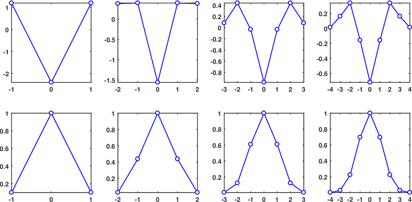
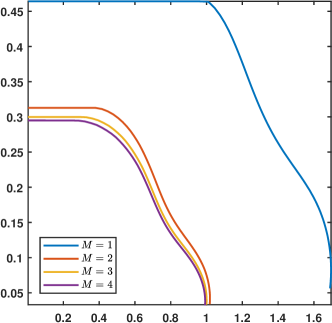
Fig.1 shows the solution of the optimization problem Eq.(20) for approximating second derivative with fourth order accuracy, for various stencil sizes. As shown in Lemma 2, both 𝐚d\mathbf{a}_{d}^{*} and 𝐛d\mathbf{b}_{d}^{*} are symmetric about the central element. Numerical values of the coefficients are tabulated in Table 1 in Appendix B.

Note that, for M=1M=1, there is no degree of freedom in the system for optimization. Consequently, for this case we recover the non-optimized standard scheme. In other words, 𝓞11(4)\boldsymbol{\mathcal{O}}^{1}_{1}(4) is identical to the non-optimized 𝓢11(4)\boldsymbol{\mathcal{S}}^{1}_{1}(4).

Refer to caption
Figure 1: Optimal stencil coefficients for 𝓞MM(4)\boldsymbol{\mathcal{O}}^{M}_{M}(4) approximating the second derivative. γ(η)=1\gamma(\eta)=1 for η[0,3]\eta\in[0,3], and γ(η)=0\gamma(\eta)=0 otherwise.

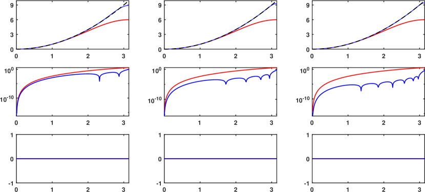
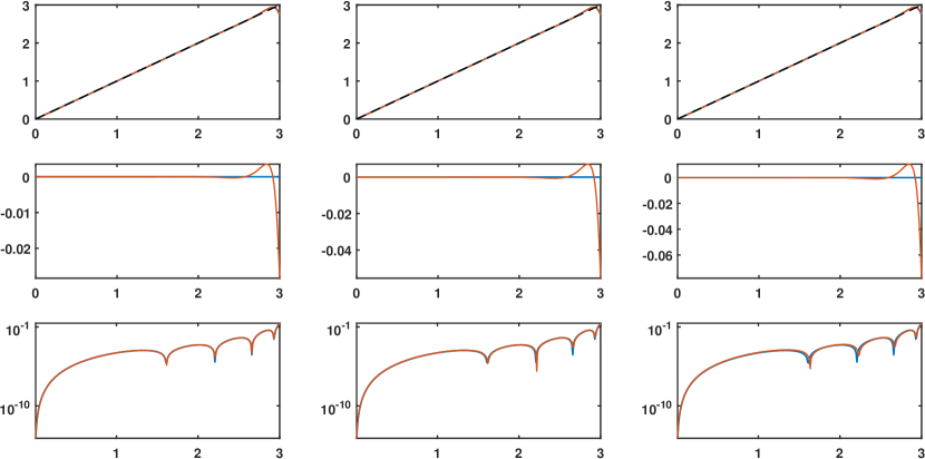
The first row of Fig.2 shows the comparison of η~2\tilde{\eta}^{2} (defined in Eq.(11)) for different values of MM (blue), with η2\eta^{2} which is calculated analytically (black dashed). In all subplots, numerical results obtained for 𝓢11(4)\boldsymbol{\mathcal{S}}^{1}_{1}(4) (red) are also shown for comparison. It is evident that, η~2\tilde{\eta}^{2} for optimized schemes is closer to analytical η2\eta^{2} than the standard scheme.

Nature of the spectral error can be further studied by analyzing real and imaginary components of e(η)e(\eta), which are shown in bottom two rows of Fig.2. For a better visualization, absolute value of the real component [e(η)]\Re[e(\eta)] is plotted in log scale. Clearly, optimized schemes (blue) have better spectral accuracy than the non-optimized standard scheme (red), especially at higher wavenumbers. The real component [e(η)]\Re[e(\eta)] is significant for optimized schemes as well. However, it decreases as MM is increased.

In accordance with Corollary 1, we observe that the imaginary component [e(η)]\Im[e(\eta)] is zero for the second derivative.

Refer to caption
Figure 2: Modified wavenumber, and real and imaginary components of spectral error for 𝓞MM(4)\boldsymbol{\mathcal{O}}^{M}_{M}(4) (blue) approximating the second derivative. γ(η)=1\gamma(\eta)=1 for η[0,3]\eta\in[0,3], and γ(η)=0\gamma(\eta)=0 otherwise. While analytical η2\eta^{2} is shown by black dashed line, red solid line shows the results for 𝓢11(4)\boldsymbol{\mathcal{S}}^{1}_{1}(4).

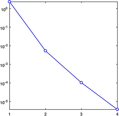
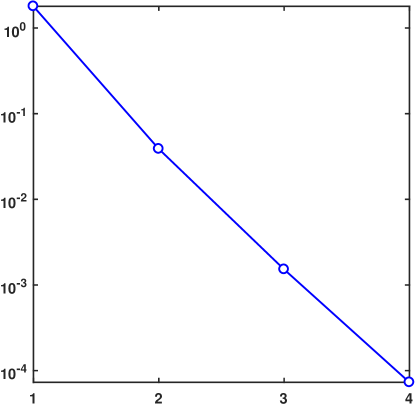
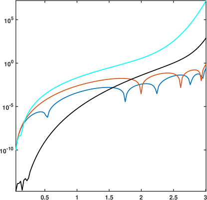
The overall effect of changing the stencil size (or MM), on the spectral error is illustrated in Fig.3. For a fixed order of accuracy, larger MM provides more freedom, and hence bigger scope of minimizing the spectral error in the optimization problem. Therefore, as expected, the spectral error decreases with increase in MM.

Refer to caption
Figure 3: 2{\mathcal{L}_{2}} norm of spectral error for 𝓞MM(4)\boldsymbol{\mathcal{O}}^{M}_{M}(4) approximating the second derivative. γ(η)=1\gamma(\eta)=1 for η[0,3]\eta\in[0,3], and γ(η)=0\gamma(\eta)=0 otherwise.

2.2 Odd derivatives

For odd dd, i.e. d:=2q+1d:=2q+1, for q={0,1,2,}q=\{0,1,2,\cdots\}, the spectral error from Eq.(10) is

e(η)=(𝐂T(η)𝐚d+(1)qηd𝐒T(η)𝐛d)+j(𝐒T(η)𝐚d(1)qηd𝐂T(η)𝐛d)(𝐂T(η)+j𝐒T(η))𝐛d.\displaystyle e(\eta)=\frac{\left(\mathbf{C}^{T}(\eta)\mathbf{a}_{d}+(-1)^{q}\eta^{d}\mathbf{S}^{T}(\eta)\mathbf{b}_{d}\right)+j\left(\mathbf{S}^{T}(\eta)\mathbf{a}_{d}-(-1)^{q}\eta^{d}\mathbf{C}^{T}(\eta)\mathbf{b}_{d}\right)}{\left(\mathbf{C}^{T}(\eta)+j\mathbf{S}^{T}(\eta)\right)\mathbf{b}_{d}}.

Using arguments similar to the case for even dd, we can minimize e(η)2\left\|e(\eta)\right\|_{\mathcal{L}_{2}} by minimizing

(𝐂T(η)𝐚d+(1)qηd𝐒T(η)𝐛d)+j(𝐒T(η)𝐚d(1)qηd𝐂T(η)𝐛d)2,\displaystyle\left\|\left(\mathbf{C}^{T}(\eta)\mathbf{a}_{d}+(-1)^{q}\eta^{d}\mathbf{S}^{T}(\eta)\mathbf{b}_{d}\right)+j\left(\mathbf{S}^{T}(\eta)\mathbf{a}_{d}-(-1)^{q}\eta^{d}\mathbf{C}^{T}(\eta)\mathbf{b}_{d}\right)\right\|_{\mathcal{L}_{2}},
=(𝐚d𝐛d)T𝐐d(𝐚d𝐛d),\displaystyle=\begin{pmatrix}\mathbf{a}_{d}\\ \mathbf{b}_{d}\end{pmatrix}^{T}\mathbf{Q}_{d}\begin{pmatrix}\mathbf{a}_{d}\\ \mathbf{b}_{d}\end{pmatrix},

where

𝐐d=[𝐂(η)(1)qηd𝐒(η)][𝐂(η)(1)qηd𝐒(η)]T+[𝐒(η)(1)qηd𝐂(η)][𝐒(η)(1)qηd𝐂(η)]T.\displaystyle\mathbf{Q}_{d}=\left\langle\begin{bmatrix}\mathbf{C}(\eta)\\ (-1)^{q}\eta^{d}\mathbf{S}(\eta)\end{bmatrix}\begin{bmatrix}\mathbf{C}(\eta)\\ (-1)^{q}\eta^{d}\mathbf{S}(\eta)\end{bmatrix}^{T}+\begin{bmatrix}\mathbf{S}(\eta)\\ -(-1)^{q}\eta^{d}\mathbf{C}(\eta)\end{bmatrix}\begin{bmatrix}\mathbf{S}(\eta)\\ -(-1)^{q}\eta^{d}\mathbf{C}(\eta)\end{bmatrix}^{T}\right\rangle. (33)

The optimization problem is the same as Eq.(20), with 𝐐d\mathbf{Q}_{d} defined by Eq.(33), and the analytical solution is given by Eq.(2.1).

Symmetry or skew-symmetry of optimal coefficients obtained for odd derivatives is justified by the following lemma. And its effect on the spectral error is discussed in Corollary 2.

Lemma 3.

In case of odd derivatives, optimal coefficients, 𝐚d\mathbf{a}_{d}^{*} and 𝐛d\mathbf{b}_{d}^{*} are respectively, skew-symmetric and symmetric about the central element.

Proof.

For odd derivatives, the integrand function is

g(𝐚d,𝐛d)=γ(η)[(𝐂T(η)𝐚d+(1)qηd𝐒T(η)𝐛d)2+(𝐒T(η)𝐚d(1)qηd𝐂T(η)𝐛d)2].\displaystyle g(\mathbf{a}_{d},\mathbf{b}_{d})=\gamma(\eta)\left[\left(\mathbf{C}^{T}(\eta)\mathbf{a}_{d}+(-1)^{q}\eta^{d}\mathbf{S}^{T}(\eta)\mathbf{b}_{d}\right)^{2}+\left(\mathbf{S}^{T}(\eta)\mathbf{a}_{d}-(-1)^{q}\eta^{d}\mathbf{C}^{T}(\eta)\mathbf{b}_{d}\right)^{2}\right].

Using similar arguments as for the case of even derivatives, it can be easily shown that,

g(𝐉𝐚d,𝐉𝐛d)=g(𝐚d,𝐛d).\displaystyle g(-\mathbf{J}\mathbf{a}_{d},\mathbf{J}\mathbf{b}_{d})=g(\mathbf{a}_{d},\mathbf{b}_{d}).

If (𝐚d,𝐛d)(\mathbf{a}_{d}^{*},\mathbf{b}_{d}^{*}) is the unique optimal solution, then

𝐉𝐚d=𝐚dand𝐉𝐛d=𝐛d.\displaystyle-\mathbf{J}\mathbf{a}_{d}^{*}=\mathbf{a}_{d}^{*}\quad\text{and}\quad\mathbf{J}\mathbf{b}_{d}^{*}=\mathbf{b}_{d}^{*}. (34)

By definition, 𝐚d\mathbf{a}_{d}^{*} and 𝐛d\mathbf{b}_{d}^{*} are respectively skew-symmetric and symmetric about the central element. To show that this solution satisfies order of accuracy constraints, consider Eq.(31). Now, substitute (𝐚d,𝐛d)(\mathbf{a}_{d},\mathbf{b}_{d}) with (𝐉𝐚d,𝐉𝐛d)(-\mathbf{J}\mathbf{a}_{d},\mathbf{J}\mathbf{b}_{d}) to get,

𝐚dT𝐉T𝐗d𝐛dT𝐉T𝐘d=𝟎1×(d+p+1).\displaystyle-\mathbf{a}_{d}^{T}\mathbf{J}^{T}\mathbf{X}_{d}-\mathbf{b}_{d}^{T}\mathbf{J}^{T}\mathbf{Y}_{d}=\mathbf{0}_{1\times(d+p+1)}.

Using the similar arguments as for the case of even derivative given in Lemma (2), it can be shown that if (𝐚d,𝐛d)(\mathbf{a}_{d},\mathbf{b}_{d}) satisfies Eq.(31), then (𝐉𝐚d,𝐉𝐛d)(-\mathbf{J}\mathbf{a}_{d},\mathbf{J}\mathbf{b}_{d}) also satisfies the same constraint for odd dd. Therefore, (𝐚d,𝐛d)(\mathbf{a}_{d}^{*},\mathbf{b}_{d}^{*}) which satisfy Eq.(34) is a feasible solution for Eq.(31). ∎

Corollary 2.

For odd derivatives, real component of the spectral error is zero.

Proof.

Multiplying first sub-equation of Eq.(34) by 𝐂T(η)\mathbf{C}^{T}(\eta) and the second by 𝐒T(η)\mathbf{S}^{T}(\eta) and using Eq.(13), we get,

𝐂T(η)𝐚d=0and𝐒T(η)𝐛d=0.\displaystyle\mathbf{C}^{T}(\eta)\mathbf{a}_{d}^{*}=0\quad\text{and}\quad\mathbf{S}^{T}(\eta)\mathbf{b}_{d}^{*}=0. (35)

Thus, spectral error from Eq.(10) becomes,

e(η)=j(𝐒T(η)𝐚d𝐂T(η)𝐛d(1)qηd).\displaystyle e(\eta)=j\bigg(\frac{\mathbf{S}^{T}(\eta)\mathbf{a}_{d}^{*}}{\mathbf{C}^{T}(\eta)\mathbf{b}_{d}^{*}}-(-1)^{q}\eta^{d}\bigg).

Therefore, for odd derivatives, optimal coefficients make real component of the spectral error e(η)e(\eta) zero. ∎

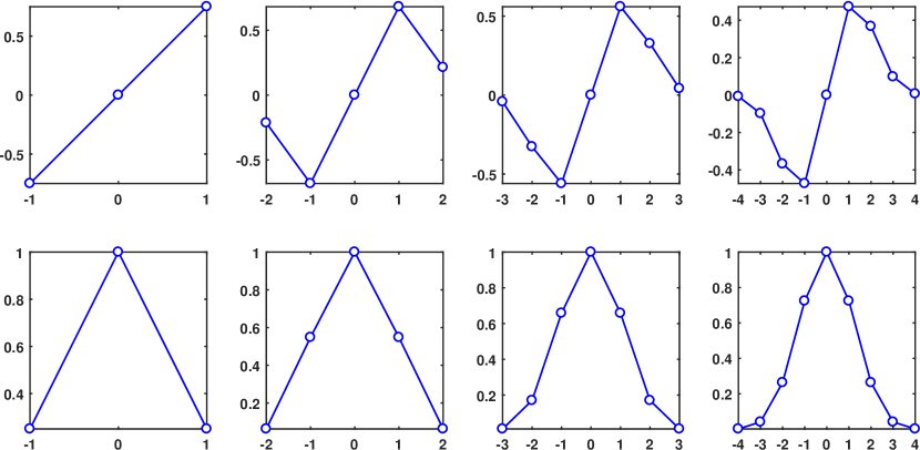
Fig.4 shows the solution of the optimization problem Eq.(20) for approximating first derivative with fourth order accuracy, for various stencil sizes. As shown in Lemma 3, 𝐚d\mathbf{a}_{d}^{*} and 𝐛d\mathbf{b}_{d}^{*} are respectively, skew-symmetric and symmetric about the central element. Numerical values of the coefficients are tabulated in Table 2. As in the case of second derivative, here also we recover the standard non-optimized scheme, 𝓢11(4)\boldsymbol{\mathcal{S}}^{1}_{1}(4), for M=1M=1.

Refer to caption
Figure 4: Optimal stencil coefficients for 𝓞MM(4)\boldsymbol{\mathcal{O}}^{M}_{M}(4) approximating the first derivative. γ(η)=1\gamma(\eta)=1 for η[0,3]\eta\in[0,3], and γ(η)=0\gamma(\eta)=0 otherwise.

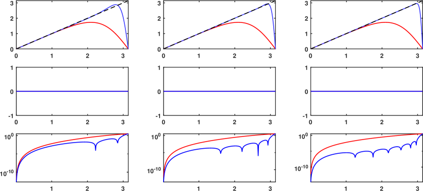
Again, as in the case of second derivative, similar observations are made for the spectral accuracy of optimized schemes approximating the first derivative. The top row of Fig.5 shows the clear advantage of optimized schemes (blue) over the standard scheme (red). While the absolute value of imaginary component [e(η)]\Im[e(\eta)] (shown in log scale) decreases with increasing MM, the real component [e(η)]\Re[e(\eta)], as expected from Corollary 2, is zero for the first derivative. Similar to Fig.3, Fig.6 also shows that as MM increases, the spectral error decreases.

Although the current framework has been derived for any positive integer MM, we observed empirically that KKT matrix in Eq.(2.1) becomes rank deficient for M6M\geq 6 and η[0,3]\eta\in[0,3], i.e., its inverse does not exist and we cannot determine optimal coefficients analytically. We also observed that the minimum MM at which KKT matrix becomes rank deficient depends on the range of η\eta. However, explicit schemes discussed in Section 4.2 do not suffer from this problem. We intend to theoretically investigate this issue in our future work.

Next, we consider the effect of γ(η)\gamma(\eta) on spectral accuracy of optimized schemes.
Refer to caption
Figure 5: Modified wavenumber, and real and imaginary components of spectral error for 𝓞MM(4)\boldsymbol{\mathcal{O}}^{M}_{M}(4) (blue) approximating the first derivative. γ(η)=1\gamma(\eta)=1 for η[0,3]\eta\in[0,3], and γ(η)=0\gamma(\eta)=0 otherwise. While analytical η\eta is shown by black dashed line, red solid line shows the results for 𝓢11(4)\boldsymbol{\mathcal{S}}^{1}_{1}(4).
Refer to caption
Figure 6: 2{\mathcal{L}_{2}} norm of spectral error for 𝓞MM(4)\boldsymbol{\mathcal{O}}^{M}_{M}(4) approximating the first derivative. γ(η)=1\gamma(\eta)=1 for η[0,3]\eta\in[0,3], and γ(η)=0\gamma(\eta)=0 otherwise.

2.3 Effect of γ(η)\gamma(\eta)

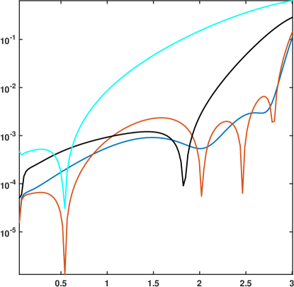
Recall that we used weighting function γ(η)0\gamma(\eta)\geq 0 when we defined 2{\mathcal{L}_{2}}-norm of error in Eq.(12). In the optimal solutions presented so far, we have used γ(η)=1\gamma(\eta)=1 for η[0,3]\eta\in[0,3] and γ(η)=0\gamma(\eta)=0 otherwise. i.e. equal weightage was given to all wavenumbers within [0,3][0,3]. We can use γ(η)\gamma(\eta) to weight some preferred wavenumbers more than others and can be selected based upon physics involved in the PDE being solved. This essentially means that, we can keep the error low at preferred wavenumbers at the expense of higher errors at other wavenumbers that are not vital to the physics of problem.

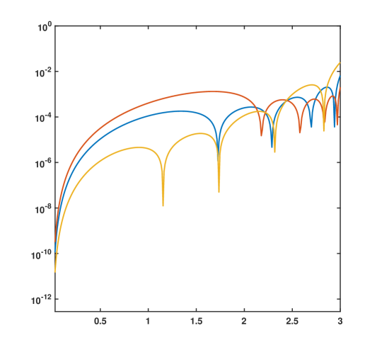
To study the effect of weighting function on spectral behavior of optimized schemes, let us consider a candidate function γ(η)=exp(αη)0\gamma(\eta)=\exp(\alpha\eta)\geq 0 where α\alpha\in\mathbb{R}. By choosing different values of α\alpha, one can assign different weightage for different wavenumbers. For example, α<0\alpha<0 weights lower wavenumbers more than the higher ones, α=0\alpha=0 i.e., γ(η)=1\gamma(\eta)=1 weights all wavenumbers equally, and α>0\alpha>0 weights higher wavenumbers more that the lower ones. This spectral behavior of optimized schemes is illustrated in Fig.7.
Refer to caption
Figure 7: Spectral error for 𝓞33(4)\boldsymbol{\mathcal{O}}^{3}_{3}(4) approximating second derivative for γ(η)=1\gamma(\eta)=1 – blue; γ(η)=exp(6η)\gamma(\eta)=\exp(6\eta) – red; γ(η)=exp(6η)\gamma(\eta)=\exp(-6\eta) – yellow, for η[0,3]\eta\in[0,3], and γ(η)=0\gamma(\eta)=0 otherwise.

The choice of exponential for weighting function is purely for the purpose of illustration in Fig.7. One can also weight wavenumbers only over finite number of intervals, e.g., γ(η)=sin(η)\gamma(\eta)=\sin(\eta) for η[0,1]\eta\in[0,1], γ(η)=1\gamma(\eta)=1 for η[2,3]\eta\in[2,3], and γ(η)=0\gamma(\eta)=0 otherwise. From this discussion it is evident that, the flexibility of choosing γ(η)\gamma(\eta) can be leveraged to improve the accuracy of solution at wavenumbers that are relevant to the physics of problem.

The unified framework presented in this section allows us to derive central compact schemes with specified order of accuracy. The schemes are also optimized using γ(η)\gamma(\eta) to have desired spectral accuracy over the wavenumber space. The third important aspect of discretization, in addition to order of accuracy and spectral error, is the temporal stability, which is discussed next. But, before proceeding further, we make the following observation that is used in the stability analysis.

The optimal coefficients for ithi^{\text{th}} grid point are derived using Eq.(2). Since ii is arbitrary, it is clear that optimal coefficients must be identical for all ii in the domain. For the sake of completeness, the formal proof for the same is presented as Lemma 4 in Appendix A.

3 Stability

Let us consider the general linear partial differential equation

ft=d=1Dβddfdx.\displaystyle\frac{\partial f}{\partial t}=\sum_{d=1}^{D}\beta_{d}\frac{\partial^{d}f}{\partial^{d}x}. (36)

Let the coefficients for the dthd^{\text{th}} derivative at the ithi^{\text{th}} grid point be parameterized by 𝐚i,d{\mathbf{a}}_{i,d} and 𝐛i,d{\mathbf{b}}_{i,d}, and 𝐀d\mathbf{A}_{d} and 𝐁d\mathbf{B}_{d} be the vertical stacking of 𝐚i,dT\mathbf{a}^{T}_{i,d} and 𝐛i,dT\mathbf{b}^{T}_{i,d} respectively, i.e.

𝐀d:=[𝐚1,dT𝐚Np,dT],𝐁d:=[𝐛1,dT𝐛Np,dT],\displaystyle\mathbf{A}_{d}:=\begin{bmatrix}{\mathbf{a}}_{1,d}^{T}\\ \vdots\\ {\mathbf{a}}_{N_{p},d}^{T}\end{bmatrix},\;\mathbf{B}_{d}:=\begin{bmatrix}{\mathbf{b}}_{1,d}^{T}\\ \vdots\\ {\mathbf{b}}_{N_{p},d}^{T}\end{bmatrix}, (37)

where NpN_{p} is the total number of grid points in the domain. We next introduce a shift operator 𝚽k\mathbf{\Phi}_{k}, which is an Np×NpN_{p}\times N_{p} matrix with elements

Φkij:=δ((ijk)modNp),\displaystyle\Phi_{k_{ij}}:=\delta((i-j-k)\mod N_{p}),

where δ()\delta(\cdot) is the Kronecker delta function defined in Eq.(2.1). When applied to a vector, the operator 𝚽k\mathbf{\Phi}_{k} cyclically shifts the elements in the vector kk times. For example,

𝚽1:=δ((ij1)mod4)=[0001100001000010],𝐯:=[1234].\mathbf{\Phi}_{1}:=\delta((i-j-1)\mod 4)=\begin{bmatrix}0&0&0&1\\ 1&0&0&0\\ 0&1&0&0\\ 0&0&1&0\end{bmatrix},\quad\mathbf{v}:=\begin{bmatrix}1\\ 2\\ 3\\ 4\end{bmatrix}.

Then,

𝚽1𝐯=[4123],and𝐯T𝚽1=[2341].\mathbf{\Phi}_{1}\mathbf{v}=\begin{bmatrix}4\\ 1\\ 2\\ 3\end{bmatrix},\quad\text{and}\quad\mathbf{v}^{T}\mathbf{\Phi}_{1}=\begin{bmatrix}2&3&4&1\end{bmatrix}.

Let 𝐀d𝚽\mathbf{A}_{d}^{\mathbf{\Phi}} and 𝐁d𝚽\mathbf{B}_{d}^{\mathbf{\Phi}} be the vertical stacking of 𝐚i,dT𝚽Mi+1{\mathbf{a}}^{T}_{i,d}\mathbf{\Phi}_{M-i+1} and 𝐛i,dT𝚽Mi+1{\mathbf{b}}^{T}_{i,d}\mathbf{\Phi}_{M-i+1} respectively, i.e.

𝐀d𝚽:=[𝐚1,dT𝚽M𝐚Np,dT𝚽M],𝐁d𝚽:=[𝐛1,dT𝚽M𝐛Np,dT𝚽M],\displaystyle\mathbf{A}_{d}^{\mathbf{\Phi}}:=\begin{bmatrix}{\mathbf{a}}_{1,d}^{T}\mathbf{\Phi}_{M}\\ \vdots\\ {\mathbf{a}}_{N_{p},d}^{T}\mathbf{\Phi}_{-M}\end{bmatrix},\;\mathbf{B}_{d}^{\mathbf{\Phi}}:=\begin{bmatrix}{\mathbf{b}}_{1,d}^{T}\mathbf{\Phi}_{M}\\ \vdots\\ {\mathbf{b}}_{N_{p},d}^{T}\mathbf{\Phi}_{-M}\end{bmatrix}, (38)

Therefore, we can write

𝐀d𝚽=i=1Np𝜹Np(i)𝜹Np(i)T𝐀d𝚽Mi+1,\displaystyle\mathbf{A}_{d}^{\mathbf{\Phi}}=\sum_{i=1}^{N_{p}}\boldsymbol{\delta}_{N_{p}}(i)\boldsymbol{\delta}_{N_{p}}(i)^{T}\mathbf{A}_{d}\mathbf{\Phi}_{M-i+1}, (39)
𝐁d𝚽=i=1Np𝜹Np(i)𝜹Np(i)T𝐁d𝚽Mi+1.\displaystyle\mathbf{B}_{d}^{\mathbf{\Phi}}=\sum_{i=1}^{N_{p}}\boldsymbol{\delta}_{N_{p}}(i)\boldsymbol{\delta}_{N_{p}}(i)^{T}\mathbf{B}_{d}\mathbf{\Phi}_{M-i+1}. (40)

where, 𝜹Np()Np\boldsymbol{\delta}_{N_{p}}(\cdot)\in\mathbb{R}^{N_{p}}, as defined in Eq.(17). Thus, 𝐀d𝚽\mathbf{A}_{d}^{\mathbf{\Phi}} and 𝐁d𝚽\mathbf{B}_{d}^{\mathbf{\Phi}} are linear functions of 𝐀d\mathbf{A}_{d} and 𝐁d\mathbf{B}_{d} defined in Eq.(37). Let us define two vectors,

𝐅:=[f1fNp],and𝐅(d):=[f1(d)fNp(d)].\displaystyle\mathbf{F}:=\begin{bmatrix}f_{1}\\ \vdots\\ f_{N_{p}}\end{bmatrix},\quad\text{and}\quad\mathbf{F}^{(d)}:=\begin{bmatrix}f_{1}^{(d)}\\ \vdots\\ f_{N_{p}}^{(d)}\end{bmatrix}.

The finite-difference approximation for the dthd^{\text{th}} derivative at the ithi^{\text{th}} grid point is

𝐛i,dT𝚽Mi+1𝐅(d)=1(Δx)d𝐚i,dT𝚽Mi+1𝐅,\displaystyle{\mathbf{b}}^{T}_{i,d}\mathbf{\Phi}_{M-i+1}\mathbf{F}^{(d)}=\frac{1}{(\Delta x)^{d}}{\mathbf{a}}_{i,d}^{T}\mathbf{\Phi}_{M-i+1}\mathbf{F},

for i={1,2,,Np}i=\{1,2,\cdots,N_{p}\}. The finite-difference approximation for the dthd^{\text{th}} derivative over the entire domain is therefore

𝐁d𝚽𝐅(d)=1(Δx)d𝐀d𝚽𝐅,\displaystyle\mathbf{B}_{d}^{\mathbf{\Phi}}\mathbf{F}^{(d)}=\frac{1}{(\Delta x)^{d}}\mathbf{A}_{d}^{\mathbf{\Phi}}\mathbf{F},

or,

𝐅(d)=1(Δx)d(𝐁d𝚽)1𝐀d𝚽𝐅.\displaystyle\mathbf{F}^{(d)}=\frac{1}{(\Delta x)^{d}}(\mathbf{B}_{d}^{\mathbf{\Phi}})^{-1}\mathbf{A}_{d}^{\mathbf{\Phi}}\mathbf{F}. (41)

subject to the existence of the inverse. For all the schemes presented in this paper, 𝐁d𝚽\mathbf{B}_{d}^{\mathbf{\Phi}} turns out to be invertible.

3.1 Stability of semi-discrete scheme

Similar to the stability analysis presented in [1] for explicit spatial schemes, herein we generalize it for implicit schemes. Using spatial discretization Eq.(41), we can convert PDE Eq.(36) into an ODE which is continuous in time as follows

𝐅˙=(d=1D1(Δx)dβd(𝐁d𝚽)1𝐀d𝚽)𝚲:=𝐅=𝚲𝐅,\displaystyle\mathbf{\dot{F}}=\underbrace{\bigg(\sum_{d=1}^{D}\frac{1}{(\Delta x)^{d}}\beta_{d}(\mathbf{B}_{d}^{\mathbf{\Phi}})^{-1}\mathbf{A}_{d}^{\mathbf{\Phi}}\bigg)}_{\mathbf{\Lambda}:=}\mathbf{F}=\mathbf{\Lambda}\mathbf{F}, (42)

with solution

𝐅(t)=exp(t𝚲)𝐅𝟎,\displaystyle\mathbf{F}(t)=\exp(t\mathbf{\Lambda})\mathbf{F_{0}}, (43)

where 𝐅𝟎\mathbf{F_{0}} is the initial condition. For a single Fourier mode, the approximate dthd^{\text{th}} derivative can be expressed in terms of the modified wavenumber as (jη~)df^(j\tilde{\eta})^{d}\hat{f}. Then the original PDE becomes,

df^dt=d=1Dβd(jη~)df^.\displaystyle\frac{d\hat{f}}{dt}=\sum_{d=1}^{D}\beta_{d}(j\tilde{\eta})^{d}\hat{f}.

The solution is given by

f^f0^=exp[d=1Dβd(jη~)dt],\displaystyle\frac{\hat{f}}{\hat{f_{0}}}=\exp\left[\sum_{d=1}^{D}\beta_{d}(j\tilde{\eta})^{d}t\right],

where f0^\hat{f_{0}} is the initial condition at t=0t=0. If the solution to the original PDE is non-increasing in time, then the discretization is considered stable if no Fourier mode grows in time. This is satisfied if

{d=1Dβd(jη~)d}0.\displaystyle\Re\left\{\sum_{d=1}^{D}\beta_{d}(j\tilde{\eta})^{d}\right\}\leq 0. (44)

From Lemma 2 and 3, and equation Eq.(10),

(jη~)d\displaystyle(j\tilde{\eta})^{d} =𝐂T(η)𝐚d𝐂T(η)𝐛d,for even d, and\displaystyle=\frac{\mathbf{C}^{T}(\eta)\mathbf{a}_{d}}{\mathbf{C}^{T}(\eta)\mathbf{b}_{d}},\quad\text{for even $d$, and}
(jη~)d\displaystyle(j\tilde{\eta})^{d} =j(𝐒T(η)𝐚d𝐂T(η)𝐛d),for odd d.\displaystyle=j\bigg(\frac{\mathbf{S}^{T}(\eta)\mathbf{a}_{d}}{\mathbf{C}^{T}(\eta)\mathbf{b}_{d}}\bigg),\quad\text{for odd $d$.}

Therefore,

d=1Dβd(jη~)d\displaystyle\sum_{d=1}^{D}\beta_{d}(j\tilde{\eta})^{d} =jβ1𝐒T(η)𝐚1𝐂T(η)𝐛1+β2𝐂T(η)𝐚2𝐂T(η)𝐛2+jβ3𝐒T(η)𝐚3𝐂T(η)𝐛3+β4𝐂T(η)𝐚4𝐂T(η)𝐛4\displaystyle=j\beta_{1}\frac{\mathbf{S}^{T}(\eta)\mathbf{a}_{1}}{\mathbf{C}^{T}(\eta)\mathbf{b}_{1}}+\beta_{2}\frac{\mathbf{C}^{T}(\eta)\mathbf{a}_{2}}{\mathbf{C}^{T}(\eta)\mathbf{b}_{2}}+j\beta_{3}\frac{\mathbf{S}^{T}(\eta)\mathbf{a}_{3}}{\mathbf{C}^{T}(\eta)\mathbf{b}_{3}}+\beta_{4}\frac{\mathbf{C}^{T}(\eta)\mathbf{a}_{4}}{\mathbf{C}^{T}(\eta)\mathbf{b}_{4}}...
=(β2𝐂T(η)𝐚2𝐂T(η)𝐛2+β4𝐂T(η)𝐚4𝐂T(η)𝐛4+)+j(β1𝐒T(η)𝐚1𝐂T(η)𝐛1+β3𝐒T(η)𝐚3𝐂T(η)𝐛3+)\displaystyle=(\beta_{2}\frac{\mathbf{C}^{T}(\eta)\mathbf{a}_{2}}{\mathbf{C}^{T}(\eta)\mathbf{b}_{2}}+\beta_{4}\frac{\mathbf{C}^{T}(\eta)\mathbf{a}_{4}}{\mathbf{C}^{T}(\eta)\mathbf{b}_{4}}+...)+j(\beta_{1}\frac{\mathbf{S}^{T}(\eta)\mathbf{a}_{1}}{\mathbf{C}^{T}(\eta)\mathbf{b}_{1}}+\beta_{3}\frac{\mathbf{S}^{T}(\eta)\mathbf{a}_{3}}{\mathbf{C}^{T}(\eta)\mathbf{b}_{3}}+...)

Then Eq.(44) implies,

{d=1Dβd(jη~)d}=β2𝐂T(η)𝐚2𝐂T(η)𝐛2+β4𝐂T(η)𝐚4𝐂T(η)𝐛4+0.\displaystyle\Re\left\{\sum_{d=1}^{D}\beta_{d}(j\tilde{\eta})^{d}\right\}=\beta_{2}\frac{\mathbf{C}^{T}(\eta)\mathbf{a}_{2}}{\mathbf{C}^{T}(\eta)\mathbf{b}_{2}}+\beta_{4}\frac{\mathbf{C}^{T}(\eta)\mathbf{a}_{4}}{\mathbf{C}^{T}(\eta)\mathbf{b}_{4}}+...\leq 0. (45)

For even dd, i.e. d=2qd=2q, the optimization of spectral error guarantees,

(jη~)d=(1)qη~2q=𝐂T(η)𝐚2q𝐂T(η)𝐛2q.\displaystyle(j\tilde{\eta})^{d}=(-1)^{q}\tilde{\eta}^{2q}=\frac{\mathbf{C}^{T}(\eta)\mathbf{a}_{2q}}{\mathbf{C}^{T}(\eta)\mathbf{b}_{2q}}.

Therefore, the sign of 𝐂T(η)𝐚2q𝐂T(η)𝐛2q\frac{\mathbf{C}^{T}(\eta)\mathbf{a}_{2q}}{\mathbf{C}^{T}(\eta)\mathbf{b}_{2q}} changes alternatively with qq as follows,

for q=1,𝐂T(η)𝐚2𝐂T(η)𝐛2\displaystyle\text{for $q=1$,}\quad\frac{\mathbf{C}^{T}(\eta)\mathbf{a}_{2}}{\mathbf{C}^{T}(\eta)\mathbf{b}_{2}} =η~20,\displaystyle=-\tilde{\eta}^{2}\leq 0,
for q=2,𝐂T(η)𝐚4𝐂T(η)𝐛4\displaystyle\text{for $q=2$,}\quad\frac{\mathbf{C}^{T}(\eta)\mathbf{a}_{4}}{\mathbf{C}^{T}(\eta)\mathbf{b}_{4}} =η~40,\displaystyle=\tilde{\eta}^{4}\geq 0,
for q=3,𝐂T(η)𝐚6𝐂T(η)𝐛6\displaystyle\text{for $q=3$,}\quad\frac{\mathbf{C}^{T}(\eta)\mathbf{a}_{6}}{\mathbf{C}^{T}(\eta)\mathbf{b}_{6}} =η~60,\displaystyle=-\tilde{\eta}^{6}\leq 0,

and so on. If coefficients βd\beta_{d} for d=2qd=2q satisfy β2q=(1)q+1ζ2q2\beta_{2q}=(-1)^{q+1}\zeta_{2q}^{2} for ζ2q\zeta_{2q}\in\mathbb{R}, then Eq.(45) is implicitly satisfied. In general, if

β2η~2+β4η~4β6η~6+0,\displaystyle-\beta_{2}\tilde{\eta}^{2}+\beta_{4}\tilde{\eta}^{4}-\beta_{6}\tilde{\eta}^{6}+...\leq 0, (46)

then the overall discretization is stable.

3.2 Stability of fully discretized scheme

After temporal discretization of Eq.(42) using a given temporal scheme, we get a fully discretized system. We analyze the stability of such system in this section. Our goal is to find maximum Δt\Delta t for which the overall discretization is stable. We begin with the forward Euler method.

3.2.1 Forward Euler method

Using forward Euler method for f/t\partial f/\partial t and the optimal finite difference approximation for df/xd\partial^{d}f/\partial x^{d}, from Eq.(42) we get following

𝐅k+1=(𝐈Np+d=1DΔt(Δx)dβd(𝐁d𝚽)1𝐀d𝚽)𝐅k.\displaystyle\mathbf{F}^{k+1}=\left(\mathbf{I}_{N_{p}}+\sum_{d=1}^{D}\frac{\Delta t}{(\Delta x)^{d}}\beta_{d}(\mathbf{B}_{d}^{\mathbf{\Phi}})^{-1}\mathbf{A}_{d}^{\mathbf{\Phi}}\right)\mathbf{F}^{k}. (47)

This is a linear discrete-time system in 𝐅\mathbf{F}, where the system matrix is dependent on the stencil coefficients 𝐀d\mathbf{A}_{d} and 𝐁d\mathbf{B}_{d}. For stability, the eigenvalues of (𝐈Np+Δtd1(Δx)dβd(𝐁d𝚽)1𝐀d𝚽)\left(\mathbf{I}_{N_{p}}+\Delta t\sum_{d}\frac{1}{(\Delta x)^{d}}\beta_{d}(\mathbf{B}_{d}^{\mathbf{\Phi}})^{-1}\mathbf{A}_{d}^{\mathbf{\Phi}}\right) should be less than one, which can be achieved by constraining the 22-norm as

𝐈Np+Δtd=1D1(Δx)dβd(𝐁d𝚽)1𝐀d𝚽21.\displaystyle\left\|\mathbf{I}_{N_{p}}+\Delta t\sum_{d=1}^{D}\frac{1}{(\Delta x)^{d}}\beta_{d}(\mathbf{B}_{d}^{\mathbf{\Phi}})^{-1}\mathbf{A}_{d}^{\mathbf{\Phi}}\right\|_{2}\leq 1. (48)

We use the analytical solution for 𝐀d\mathbf{A}_{d} and 𝐁d\mathbf{B}_{d} from spectral error optimization, and maximize Δt\Delta t subject to the stability constraint Eq.(48). The reader is referred to [1] for the solution of this maximization problem using software packages such as cvx [13]. Solving optimization problem by this approach may become difficult if temporal schemes other than forward Euler method are used. Therefore, we present an approach to determine maximum Δt\Delta t for generalized temporal schemes in the following section.

3.2.2 Generalized temporal scheme

Runge-Kutta (RK) methods are widely used for temporal discretization of ODEs to attain higher order of accuracy. Many temporal schemes can be expressed as special cases of implicit RK method, e.g., see Appendix C for different temporal schemes written in Butcher tableau form of RK methods. Thus, herein, we consider implicit RK method as a generalized temporal scheme to determine maximum Δt\Delta t which guarantees the stability. An implicit s\mathit{s}-stage RK scheme with the following Butcher tableau

𝒄𝑨𝒃T:=c1a11a12a1sc2a21a22a2scsas1as2a𝑠𝑠b1b2bs\displaystyle\begin{array}[]{c|c}\boldsymbol{\mathit{c}}&\boldsymbol{\mathit{A}}\\ \hline\cr&\boldsymbol{\mathit{b}}^{T}\end{array}:=\begin{array}[]{c|c c c c}\mathit{c}_{1}&\mathit{a}_{11}&\mathit{a}_{12}&\dots&\mathit{a}_{1\mathit{s}}\\ \mathit{c}_{2}&\mathit{a}_{21}&\mathit{a}_{22}&\dots&\mathit{a}_{2\mathit{s}}\\ \vdots&\vdots&\vdots&\ddots&\vdots\\ \mathit{c}_{\mathit{s}}&\mathit{a}_{\mathit{s}1}&\mathit{a}_{\mathit{s}2}&\dots&\mathit{a}_{\mathit{s}\mathit{s}}\\ \hline\cr&\mathit{b}_{1}&\mathit{b}_{2}&\dots&\mathit{b}_{\mathit{s}}\\ \end{array}

is given by

fn+1\displaystyle f^{n+1} =\displaystyle= fn+Δti=1sbiki,\displaystyle f^{n}+\Delta t\sum_{i=1}^{\mathit{s}}\mathit{b}_{i}k_{i}, (56)
ki=f˙(tn+ciΔt,fn+Δtj=1saijkj),\displaystyle k_{i}=\dot{f}\bigg(t_{n}+c_{i}\Delta t,\quad f^{n}+\Delta t\sum_{j=1}^{\mathit{s}}\mathit{a}_{ij}k_{j}\bigg),

where, fnf^{n} is the value of function f(t)f(t) at nthn^{th} time step and f˙(t,f)\dot{f}(t,f) is the time derivative of f(t)f(t) at time tt. For a scalar equation such as f˙=λf\dot{f}=\lambda f, fn+1f^{n+1} can be written in terms of stability function of the RK scheme r(z)r(z), zz\in\mathbb{C}, as

fn+1\displaystyle f^{n+1} =r(λΔt)fn,\displaystyle=r(\lambda\Delta t)f^{n}, (57)
where,r(z)\displaystyle\text{where,}\quad r(z) =1+z𝒃T(𝐈z𝑨)1𝟏s=det(𝐈+z(𝟏s𝒃T𝑨))det(𝐈z𝑨),\displaystyle=1+z\boldsymbol{\mathit{b}}^{T}(\mathbf{I}-z\boldsymbol{\mathit{A}})^{-1}\mathbf{1}_{\mathit{s}}=\frac{\det(\mathbf{I}+z(\mathbf{1}_{\mathit{s}}\boldsymbol{\mathit{b}}^{T}-\boldsymbol{\mathit{A}}))}{\det(\mathbf{I}-z\boldsymbol{\mathit{A}})},

and 𝟏s\mathbf{1}_{\mathit{s}} represents a column vector of dimension s\mathit{s} whose all elements are equal to 11 [14]. Thus, r(z)r(z) is a polynomial-over-polynomial function of zz. The sequence formed by Eq.(57) is bounded iff |r(z)|1|r(z)|\leq 1, which is the stability condition for the RK scheme. For all such z=λΔtz=\lambda\Delta t, and known λ\lambda, we can find bounds on Δt\Delta t such that the product λΔt\lambda\Delta t lies in the stability region of the RK scheme determined by the stability condition. The equality |r(z)|=1|r(z)|=1 defines a closed curve in the complex plane. Generally, for the explicit RK schemes, area enclosed by the stability curve defines the stability region. While in the case of implicit RK schemes, stability region may lie either inside or outside the closed curve. If stability curve is the imaginary axis itself, then the scheme is stable for all zz which lie in the left half of the complex plane. Note that, Δt>0\Delta t>0 is a real number while λ\lambda can be a complex number, so that z=λΔtz=\lambda\Delta t is complex. The timestep Δt\Delta t just scales the radius of λ\lambda while keeping the argument same in the complex plane. We are interested in finding maximum scaling Δt\Delta t for which scaled λ\lambda lies in the stability region.

As in the forward Euler case, here also we assume that 𝐀d\mathbf{A}_{d} and 𝐁d\mathbf{B}_{d} are determined analytically and hence 𝚲\mathbf{\Lambda} is known. Now, let us consider multi-dimensional semi-discrete system defined by Eq.(42). We reduce this NpN_{p}-dimensional system into NpN_{p} scalar decoupled systems using the similarity transformation. Let 𝐃\mathbf{D} be a diagonal matrix with eigenvalues of the 𝚲\mathbf{\Lambda} as its diagonal elements and 𝐌\mathbf{M} be the modal matrix with eigenvectors of 𝚲\mathbf{\Lambda} as its columns, such that 𝐃=𝐌1𝚲𝐌\mathbf{D}=\mathbf{M}^{-1}\mathbf{\Lambda}\mathbf{M}. Let us define the transformation 𝐋:=𝐌𝐅\mathbf{L}:=\mathbf{M}\mathbf{F}. Then Eq.(42) can be written as

𝐌𝐋˙\displaystyle\mathbf{M}\dot{\mathbf{L}} =𝚲𝐌𝐋,\displaystyle=\mathbf{\Lambda}\mathbf{M}\mathbf{L},
𝐋˙\displaystyle\dot{\mathbf{L}} =𝐌1𝚲𝐌𝐋=𝐃𝐋.\displaystyle=\mathbf{M}^{-1}\mathbf{\Lambda}\mathbf{M}\mathbf{L}=\mathbf{D}\mathbf{L}. (58)

Since 𝐃\mathbf{D} is diagonal, Eq.(58) represents NpN_{p} scalar systems as follows

l˙i\displaystyle\dot{l}_{i} =λili,i=1Np,\displaystyle=\lambda_{i}l_{i},\quad i=1\dots N_{p},

where λi\lambda_{i}, are NpN_{p} eigenvalues of 𝚲\mathbf{\Lambda}. The ithi^{\text{th}} scalar system can be fully discretized using the RK scheme, and from Eq.(57) it follows that

lin+1\displaystyle l_{i}^{n+1} =r(λiΔt)lin,i=1Np.\displaystyle=r(\lambda_{i}\Delta t)l_{i}^{n},\quad i=1\dots N_{p}.

For overall stability of Eq.(58), it is required that the products λiΔt\lambda_{i}\Delta t lie within stability region of the RK scheme. Thus, for known λi\lambda_{i}, bounds on Δt\Delta t can be calculated numerically to guarantee the stability of the system.
Refer to caption
Refer to caption
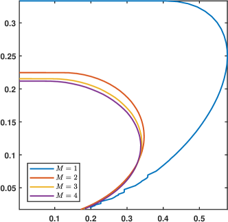
Figure 8: r2r_{2} vs r1r_{1} for forward Euler and ERK4 method. First and second derivatives approximated using 𝓞MM(4)\boldsymbol{\mathcal{O}}^{M}_{M}(4), γ(η)=1\gamma(\eta)=1 for η[0,3]\eta\in[0,3], and γ(η)=0\gamma(\eta)=0 otherwise.

Generally, Δx\Delta x and Δt\Delta t used for the complete discretization are expressed as a normalized quantity called Courant-Friedrichs-Lewy (CFL) number. The CFL number with respect to dthd^{\text{th}} derivative is defined as rd:=|βd|Δt/Δxdr_{d}:=|\beta_{d}|\Delta t/\Delta x^{d}. By varying Δx\Delta x and calculating corresponding maximum Δt\Delta t, we can calculate and plot CFL numbers r1r_{1} and r2r_{2} for the advection-diffusion equation (see Eq.(76)). A similar plot obtained for optimal schemes of different stencil sizes for forward Euler and ERK4 method is shown in Fig.8. M=1M=1 (blue) corresponds to the standard scheme 𝓢11(4)\boldsymbol{\mathcal{S}}^{1}_{1}(4), and M=2M=2 onwards correspond to optimized schemes, 𝓞MM(4)\boldsymbol{\mathcal{O}}^{M}_{M}(4). There is a drastic reduction in stability region from M=1M=1 to M=2M=2. As MM is increased further, stability region decreases.
Refer to caption
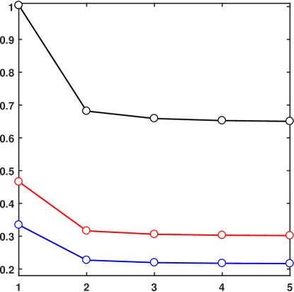
Figure 9: Variation of maximum allowable r2r_{2} with different stencil size, for different temporal schemes: FE (blue), ERK4 (red), and IRK2 (black). First and second derivatives approximated using 𝓞MM(4)\boldsymbol{\mathcal{O}}^{M}_{M}(4).
Refer to caption
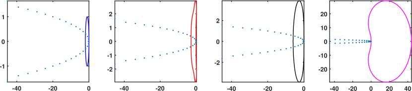
Figure 10: Closed curve shows stability regions for different RK schemes. Asterisks are eigenvalues of 𝚲\mathbf{\Lambda} for M=4M=4, β=[0.1,0.2]\beta=[-0.1,0.2], Np=31N_{p}=31. (a), (b) and (c): Inside the curve is stable. (d): Outside the curve is stable.

Variation of maximum allowable r2r_{2} with stencil size for different temporal schemes is shown in Fig.9. Butcher tableaux for the RK schemes are given in Appendix C. We observe that, for all RK schemes in Fig.9, there is a drastic drop in maximum allowable Δt\Delta t (or r2r_{2}) from M=1M=1 to M=2M=2. This is a consequence of drastic reduction in stability region from M=1M=1 to M=2M=2, similar to one shown in Fig.8. Also, maximum allowable r2r_{2} for IRK2 (black) is the largest followed by ERK4 (red) and FE (blue). This is due to the fact that IRK2 has the largest, and FE has the smallest stability region in the complex plane, as shown in Fig.10(a),(b),(c)(a),(b),(c). For the same problem specifications, IRK3 is stable for all 0<Δt<0<\Delta t<\infty, which is evident from Fig.10(d)(d), as all eigenvalues, λi\lambda_{i}, lie in the stability region of IRK3 (outside the closed curve).

We next consider the relationship between λi\lambda_{i} and the derivatives in a PDE. For even derivatives from Lemma 2, both 𝐚d\mathbf{a}_{d} and 𝐛d\mathbf{b}_{d} are symmetric about the central element. Consequently, both 𝐀d𝚽\mathbf{A}_{d}^{\mathbf{\Phi}} and 𝐁d𝚽\mathbf{B}_{d}^{\mathbf{\Phi}} defined in Eq.(38) are real symmetric circulant matrices. Therefore, if a PDE consists of only even derivatives, then 𝚲\mathbf{\Lambda} defined in Eq.(42) is also symmetric and hence all λi\lambda_{i} are real. Real parts of λi\lambda_{i} cause only amplitude decay (diffusion) or amplification but phase of the solution remains constant. On the other hand, for odd derivatives, 𝐚d\mathbf{a}_{d} is skew-symmetric and 𝐛d\mathbf{b}_{d} is symmetric about the central element. Therefore, circulant matrices 𝐀d𝚽\mathbf{A}_{d}^{\mathbf{\Phi}} and 𝐁d𝚽\mathbf{B}_{d}^{\mathbf{\Phi}} become skew-symmetric and symmetric respectively, which in turn make 𝚲\mathbf{\Lambda} a skew-symmetric matrix. Consequently, if a PDE consists of only odd derivatives, then all λi\lambda_{i} are pure imaginary which affect only phase of the solution preserving magnitude of amplitudes, leading to pure dispersion. It is clear that even derivatives contribute to the real part of λi\lambda_{i} and hence diffusion of the numerical solution, and odd derivatives cause dispersion by means of the imaginary part of λi\lambda_{i}. However, this is true only for central schemes which admit results from Lemma 2 and 3. It is shown in the subsequent section that in the case of biased schemes, both even and odd derivatives individually contribute to real and imaginary components of λi\lambda_{i}.

In what follows next, we extend the stability analysis discussed in this section, and framework presented in Section 2 to derive and analyze special types of optimized schemes.

4 Special cases of the framework

We generalize Eq.(2) further as

m=MLBMRBbmfi+m(d)=1(Δx)dm=MLAMRAamfi+m,\displaystyle\sum_{m=-M^{B}_{L}}^{M^{B}_{R}}\mathrm{b}_{m}f^{(d)}_{i+m}=\frac{1}{(\Delta x)^{d}}\sum_{m=-M^{A}_{L}}^{M^{A}_{R}}\mathrm{a}_{m}f_{i+m}, (59)

where, each one of MLB,MRB,MLAM^{B}_{L},M^{B}_{R},M^{A}_{L} and MRAM^{A}_{R} can be chosen independently. In Section 2, we have presented a general framework to derive optimal implicit finite difference approximations. These approximations are obtained for equal LHS and RHS stencil sizes, i.e. MLB=MRB=MLA=MRA=MM^{B}_{L}=M^{B}_{R}=M^{A}_{L}=M^{A}_{R}=M. In this section, we show that other types of schemes, namely, compact schemes with unequal LHS and RHS stencil sizes, spatially explicit, and biased finite difference approximations can be derived as special cases of the framework presented in Section 2. These special cases are derived by imposing additional constraints on the coefficients 𝐚𝐝\mathbf{a_{d}} and 𝐛𝐝\mathbf{b_{d}} while solving the minimization problem defined in Eq.(20).

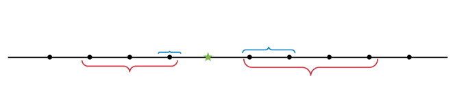
In the most generalized form, we denote (p+1)th(p+1)^{\text{th}} order accurate optimized schemes derived using Eq.(59) as 𝓞MLB,MRBMLA,MRA(p+1)\boldsymbol{\mathcal{O}}^{M^{A}_{L},M^{A}_{R}}_{M^{B}_{L},M^{B}_{R}}(p+1). For example, 5th5^{\text{th}} order accurate optimized scheme obtained using MLA=1,MRA=2,MLB=3M^{A}_{L}=1,M^{A}_{R}=2,M^{B}_{L}=3 and MRB=4M^{B}_{R}=4 is denoted by 𝓞3,41,2(5)\boldsymbol{\mathcal{O}}^{1,2}_{3,4}(5). See Fig.11 as an illustration of this. The ithi^{\text{th}} grid point at which derivative is to be approximated is shown by a green asterisk, and neighboring grid points are shown by black circles. Blue and red braces respectively show stencil points used in RHS and LHS of Eq.(59).

Refer to caption
Figure 11: Illustration for the notation of optimized schemes in the most generalized form.

4.1 Central compact schemes with unequal LHS and RHS stencil sizes

In Eq.(2), indices of both am\mathrm{a}_{m} and bm\mathrm{b}_{m} vary from M-M to MM. We can also have different ranges of index mm for am\mathrm{a}_{m} and bm\mathrm{b}_{m}. Let MLB=MRB=MBM^{B}_{L}=M^{B}_{R}=M^{B} and MLA=MRA=MAM^{A}_{L}=M^{A}_{R}=M^{A}. i.e., Eq.(59) becomes,

m=MBMBbmfi+m(d)=1(Δx)dm=MAMAamfi+m,\displaystyle\sum_{m=-M^{B}}^{M^{B}}\mathrm{b}_{m}f^{(d)}_{i+m}=\frac{1}{(\Delta x)^{d}}\sum_{m=-M^{A}}^{M^{A}}\mathrm{a}_{m}f_{i+m}, (60)

where MBMAM^{B}\neq M^{A}.

Continuing the use of the notation defined in Section 2, we refer optimized schemes derived using Eq.(60) as 𝓞MBMA()\boldsymbol{\mathcal{O}}^{M^{A}}_{M^{B}}(\cdot). On the other hand, if a scheme is derived by the standard method of coefficient matching without optimization, then it is referred by 𝓢MBMA()\boldsymbol{\mathcal{S}}^{M^{A}}_{M^{B}}(\cdot). When Eq.(1) is compared with Eq.(60), we observe that MA=3M^{A}=3 and MB=2M^{B}=2 for Eq.(1). Therefore, pentadiagonal optimized schemes are denoted by 𝓞23()\boldsymbol{\mathcal{O}}^{3}_{2}(\cdot), and pentadiagonal standard schemes are denoted by 𝓢23()\boldsymbol{\mathcal{S}}^{3}_{2}(\cdot).

The stencil size for the right side of Eq.(60) is defined as NA:=2MA+1N^{A}:=2M^{A}+1, and similarly the stencil size for the left side is NB:=2MB+1N^{B}:=2M^{B}+1. Let us define augmented parameters as M^:=max{MA,MB}\hat{M}:=\max\{M^{A},M^{B}\} and N^:=2M^+1\hat{N}:=2\hat{M}+1.

First, we consider the case MA>MBM^{A}>M^{B}, and hence M^=MA\hat{M}=M^{A}. This 𝓞MBMA()\boldsymbol{\mathcal{O}}^{M^{A}}_{M^{B}}(\cdot) scheme can be treated as an 𝓞MAMA()\boldsymbol{\mathcal{O}}^{M^{A}}_{M^{A}}(\cdot) scheme with augmented stencil size N^=NA=2MA+1\hat{N}=N^{A}=2M^{A}+1, and an extra imposed constraint that bm=0\mathrm{b}_{m}=0 for m={MA,MA+1,,(MB+1),MB+1,MB+2,,MA}m=\{-M^{A},-M^{A}+1,\cdots,-(M^{B}+1),M^{B}+1,M^{B}+2,\cdots,M^{A}\}. In other words, we are imposing a constraint that (NANB)(N^{A}-N^{B}) elements of 𝐛d\mathbf{b}_{d} which are located symmetrically about the central element, to be zero. Therefore, we can use the central difference framework presented in Section 2 with M=MAM=M^{A} and the following additional constraint

[𝜹nT(1)𝜹nT(2)𝜹nT(MAMB)𝜹nT(MA+MB+2)𝜹nT(MA+MB+3)𝜹nT(N^)]𝚫T:=𝐛d=𝟎(N^NB)×1,\displaystyle\underbrace{\begin{bmatrix}\boldsymbol{\delta}_{n}^{T}(1)\\ \boldsymbol{\delta}_{n}^{T}(2)\\ \vdots\\ \boldsymbol{\delta}_{n}^{T}(M^{A}-M^{B})\\ \boldsymbol{\delta}_{n}^{T}(M^{A}+M^{B}+2)\\ \boldsymbol{\delta}_{n}^{T}(M^{A}+M^{B}+3)\\ \vdots\\ \boldsymbol{\delta}_{n}^{T}(\hat{N})\end{bmatrix}}_{\mathbf{\Delta}^{T}:=}\mathbf{b}_{d}=\mathbf{0}_{(\hat{N}-N^{B})\times 1}, (61)

for n=N^n=\hat{N}, where 𝜹nT()\boldsymbol{\delta}_{n}^{T}(\cdot) is defined in Eq.(17). Therefore, the constraint can be written as

[𝟎(N^NB)×N^𝚫T][𝐚d𝐛d]=𝟎(N^NB)×1.\displaystyle\begin{bmatrix}\mathbf{0}_{(\hat{N}-N^{B})\times\hat{N}}&\mathbf{\Delta}^{T}\end{bmatrix}\begin{bmatrix}\mathbf{a}_{d}\\ \mathbf{b}_{d}\end{bmatrix}=\mathbf{0}_{(\hat{N}-N^{B})\times 1}. (62)

The minimization problem defined in Eq.(20) is solved analytically using the KKT condition constructed by incorporating the additional constraint Eq.(62). Then the optimal solution similar to Eq.(2.1) is given by

(𝐚d𝐛d𝝀d)=𝐏[𝟎2N^×1𝟎(d+p+1)×11𝟎(N^NB)×1],\displaystyle\begin{pmatrix}\mathbf{a}_{d}^{\ast}\\ \mathbf{b}_{d}^{\ast}\\ \boldsymbol{\lambda}_{d}^{\ast}\end{pmatrix}=\mathbf{P}\begin{bmatrix}\mathbf{0}_{2\hat{N}\times 1}\\ \mathbf{0}_{(d+p+1)\times 1}\\ 1\\ \mathbf{0}_{(\hat{N}-N^{B})\times 1}\end{bmatrix}, (63)

where,

𝐏=[𝐐d(𝐗dT𝐘dT𝟎1×N^𝜹N^T(M^+1)𝟎(N^NB)×N^𝚫T)T(𝐗dT𝐘dT𝟎1×N^𝜹N^T(M^+1)𝟎(N^NB)×N^𝚫T)𝟎(N^NB+d+p+2)×(N^NB+d+p+2)]1.\displaystyle\mathbf{P}=\left[\begin{array}[]{cc}\mathbf{Q}_{d}&\left(\begin{array}[]{cc}\mathbf{X}_{d}^{T}&-\mathbf{Y}_{d}^{T}\\ \mathbf{0}_{1\times\hat{N}}&\boldsymbol{\delta}_{\hat{N}}^{T}(\hat{M}+1)\\ \mathbf{0}_{(\hat{N}-N^{B})\times\hat{N}}&\mathbf{\Delta}^{T}\end{array}\right)^{T}\\ \left(\begin{array}[]{cc}\mathbf{X}_{d}^{T}&-\mathbf{Y}_{d}^{T}\\ \mathbf{0}_{1\times\hat{N}}&\boldsymbol{\delta}_{\hat{N}}^{T}(\hat{M}+1)\\ \mathbf{0}_{(\hat{N}-N^{B})\times\hat{N}}&\mathbf{\Delta}^{T}\end{array}\right)&\mathbf{0}_{(\hat{N}-N^{B}+d+p+2)\times(\hat{N}-N^{B}+d+p+2)}\end{array}\right]^{-1}.

In a similar manner, we can calculate optimal coefficients for the complementary case MA<MBM^{A}<M^{B} by setting (NBNA)(N^{B}-N^{A}) elements of 𝐚d\mathbf{a}_{d} to zero.

Note that by setting MA=3M^{A}=3 and MB=2M^{B}=2 in current framework, we get pentadiagonal compact schemes such as presented in [2] and [3]. Latter frameworks restrict the stencil size and require that MA>MBM^{A}>M^{B}. On the other hand, the framework presented in this paper is more general because MAM^{A} and MBM^{B} can be chosen independently.

Also note that, the constraint Eq.(61) sets bm=0\mathrm{b}_{m}=0 symmetrically about the central element of 𝐛d\mathbf{b}_{d}. Therefore, Lemmas 2 and 3, and stability analysis presented in Section 3 are valid for this special case.

4.2 Central spatially explicit schemes

A finite difference approximation is said to be spatially explicit if coefficients bmb_{m} in Eq.(2) are

bm={1 if m=0,0 if m0.\displaystyle b_{m}=\left\{\begin{array}[]{c}1\text{ if }m=0,\\ 0\text{ if }m\neq 0.\end{array}\right.

i.e.,

fi(d)=1(Δx)dm=MAMAamfi+m.\displaystyle f^{(d)}_{i}=\frac{1}{(\Delta x)^{d}}\sum_{m=-M^{A}}^{M^{A}}\mathrm{a}_{m}f_{i+m}. (64)

It is obvious that central approximations which are spatially explicit can be obtained by substituting MB=0M^{B}=0 in Eq.(60). Therefore, an optimized explicit central schemes is represented by 𝓞0MA()\boldsymbol{\mathcal{O}}^{M^{A}}_{0}(\cdot). Constraints Eq.(61) and Eq.(16) can be combined together as

[𝜹nT(1)𝜹nT(2)𝜹nT(MA+1)𝜹nT(N^1)𝜹nT(N^)]𝚫T:=𝐛d=[00100]=𝜹n(MA+1),\displaystyle\underbrace{\begin{bmatrix}\boldsymbol{\delta}_{n}^{T}(1)\\ \boldsymbol{\delta}_{n}^{T}(2)\\ \vdots\\ \boldsymbol{\delta}_{n}^{T}(M^{A}+1)\\ \vdots\\ \boldsymbol{\delta}_{n}^{T}(\hat{N}-1)\\ \boldsymbol{\delta}_{n}^{T}(\hat{N})\end{bmatrix}}_{\mathbf{\Delta}^{T}:=}\mathbf{b}_{d}=\begin{bmatrix}0\\ 0\\ \vdots\\ 1\\ \vdots\\ 0\\ 0\end{bmatrix}=\boldsymbol{\delta}_{n}(M^{A}+1), (65)

for n=N^n=\hat{N}, where N^=2MA+1\hat{N}=2M^{A}+1. Since 𝚫T\mathbf{\Delta}^{T} in the above equation is an identity matrix, the constraint reduces to

𝐛d=𝜹n(MA+1).\displaystyle\mathbf{b}_{d}=\boldsymbol{\delta}_{n}(M^{A}+1). (66)

Therefore, optimal solution can be found analytically as

(𝐚d𝐛d𝝀d)=[𝐐d(𝐗dT𝐘dT𝟎N^×N^𝐈N^×N^)T(𝐗dT𝐘dT𝟎N^×N^𝐈N^×N^)𝟎(N^+d+p+1)×(N^+d+p+1)]1[𝟎2N^×1𝟎(d+p+1)×1𝜹N^(MA+1)].\displaystyle\begin{pmatrix}\mathbf{a}_{d}^{\ast}\\ \mathbf{b}_{d}^{\ast}\\ \boldsymbol{\lambda}_{d}^{\ast}\end{pmatrix}=\left[\begin{array}[]{cc}\mathbf{Q}_{d}&\left(\begin{array}[]{cc}\mathbf{X}_{d}^{T}&-\mathbf{Y}_{d}^{T}\\ \mathbf{0}_{\hat{N}\times\hat{N}}&\mathbf{I}_{\hat{N}\times\hat{N}}\end{array}\right)^{T}\\ \left(\begin{array}[]{cc}\mathbf{X}_{d}^{T}&-\mathbf{Y}_{d}^{T}\\ \mathbf{0}_{\hat{N}\times\hat{N}}&\mathbf{I}_{\hat{N}\times\hat{N}}\end{array}\right)&\mathbf{0}_{(\hat{N}+d+p+1)\times(\hat{N}+d+p+1)}\end{array}\right]^{-1}\begin{bmatrix}\mathbf{0}_{2\hat{N}\times 1}\\ \mathbf{0}_{(d+p+1)\times 1}\\ \boldsymbol{\delta}_{\hat{N}}(M^{A}+1)\end{bmatrix}.

The only difference between spatially implicit and explicit schemes is the structure of matrix 𝐁d𝚽\mathbf{B}_{d}^{\mathbf{\Phi}}. Since in the case of explicit schemes 𝐛d\mathbf{b}_{d} is given by Eq.(65), 𝐁d𝚽\mathbf{B}_{d}^{\mathbf{\Phi}} becomes an identity matrix. Therefore stability analysis discussed in Section 3 holds true for explicit schemes as well with the substitution 𝐁d𝚽=𝐈\mathbf{B}_{d}^{\mathbf{\Phi}}=\mathbf{I} in Eq.(41).

A similar framework exclusively for spatially explicit schemes has been presented in [1] and optimal coefficients calculated using this framework match exactly with the ones obtained using Eq.(4.2). In [1], authors extensively discuss error characteristics and stability analysis for optimal explicit schemes.
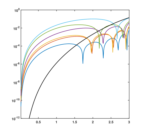
Refer to caption
Figure 12: Error in modified wavenumber for various 𝓞MBMA(4)\boldsymbol{\mathcal{O}}^{M^{A}}_{M^{B}}(4) schemes approximating second derivative. Bottom to top: Black – 𝓢23(10)\boldsymbol{\mathcal{S}}^{3}_{2}(10); blue – 𝓞33(4)\boldsymbol{\mathcal{O}}^{3}_{3}(4); red – 𝓞23(4)\boldsymbol{\mathcal{O}}^{3}_{2}(4); yellow – 𝓞32(4)\boldsymbol{\mathcal{O}}^{2}_{3}(4); purple – 𝓞13(4)\boldsymbol{\mathcal{O}}^{3}_{1}(4); green – 𝓞31(4)\boldsymbol{\mathcal{O}}^{1}_{3}(4); cyan – 𝓞03(4)\boldsymbol{\mathcal{O}}^{3}_{0}(4). N^=7\hat{N}=7, γ(η)=1\gamma(\eta)=1 for η[0,3]\eta\in[0,3], and γ(η)=0\gamma(\eta)=0 otherwise.

A comparison of η~2\tilde{\eta}^{2} with η2\eta^{2} for optimal schemes derived using different values of MAM^{A} and MBM^{B} for fixed augmented stencil size N^=7\hat{N}=7 is shown in Fig.12. It is clear that optimized scheme with equal LHS and RHS stencil sizes (MA=MBM^{A}=M^{B}), i.e. 𝓞33(4)\boldsymbol{\mathcal{O}}^{3}_{3}(4) (blue), performs better than all other optimized schemes with unequal LHS and RHS stencil sizes (MAMBM^{A}\neq M^{B}). This is expected, since 𝓞33(4)\boldsymbol{\mathcal{O}}^{3}_{3}(4) has the largest number of degrees of freedom in the optimization. We state this observation as the following remark.

Remark 1.

Among central compact optimized schemes which have same augmented stencil size, the scheme with MA=MBM^{A}=M^{B} demonstrates the best spectral accuracy.

Note that, MA>MBM^{A}>M^{B} (MA=3M^{A}=3, MB=2M^{B}=2) for 𝓞23(4)\boldsymbol{\mathcal{O}}^{3}_{2}(4) (red), and MA<MBM^{A}<M^{B} (MA=2M^{A}=2, MB=3M^{B}=3) for 𝓞32(4)\boldsymbol{\mathcal{O}}^{2}_{3}(4) (yellow). These both schemes have same number of degrees of freedom, i.e., total sum of LHS and RHS stencil sizes is same for both of them. However, from Fig.12, it can be seen that 𝓞23(4)\boldsymbol{\mathcal{O}}^{3}_{2}(4) (red) performs slightly better than 𝓞32(4)\boldsymbol{\mathcal{O}}^{2}_{3}(4) (yellow). Similarly, MA>MBM^{A}>M^{B} for 𝓞13(4)\boldsymbol{\mathcal{O}}^{3}_{1}(4) (purple), and MA<MBM^{A}<M^{B} for 𝓞31(4)\boldsymbol{\mathcal{O}}^{1}_{3}(4) (green). Clearly, 𝓞13(4)\boldsymbol{\mathcal{O}}^{3}_{1}(4) (purple) performs better than 𝓞31(4)\boldsymbol{\mathcal{O}}^{1}_{3}(4) (green). Based on these observations, we infer the following.

Remark 2.

Let M1>M2M_{1}>M_{2}. Central compact optimized schemes with MA=M1M^{A}=M_{1} and MB=M2M^{B}=M_{2} i.e., MA>MBM^{A}>M^{B}, demonstrate better spectral accuracy than those with MA=M2M^{A}=M_{2} and MB=M1M^{B}=M_{1} i.e., MA<MBM^{A}<M^{B}.

Finally, we observe that the central optimized explicit scheme 𝓞03(4)\boldsymbol{\mathcal{O}}^{3}_{0}(4) (cyan) performs worse than all other central compact optimized schemes with equal N^\hat{N}. Again, this is expected, since the explicit scheme has the minimum number of degrees of freedom in the optimization.

For the standard pentadiagonal scheme 𝓢23(10)\boldsymbol{\mathcal{S}}^{3}_{2}(10) (black), we see that the error is very small in the low wavenumber region. However, the error is large at higher wavenumbers. This leads to steep variation of error in the wavenumber space. On the other hand, the optimized pentadiagonal scheme 𝓞23(4)\boldsymbol{\mathcal{O}}^{3}_{2}(4) (red) demonstrates relatively spectrally flat behavior due to the weighting function γ(η)=1\gamma(\eta)=1, which weights all wavenumbers equally.

4.3 Biased schemes

In the discussion so far, we have assumed the domain to be periodic, which enables us to use central schemes at all grid points in the domain. Central schemes can not be used if the domain is not periodic or there are specified boundary conditions. This is because of the fact that there are unequal number of usable grid points on either side of a point which lies near boundary of the domain. Thus, we have to use one-sided or biased schemes near boundaries. A finite difference approximation is said to be biased if the number of grid points used on the left and right side of a point at which derivative is calculated is not equal. For the sake of discussion, in this special case we assume that MLB=MLA=MLM^{B}_{L}=M^{A}_{L}=M_{L} and MRB=MRA=MRM^{B}_{R}=M^{A}_{R}=M_{R}. Therefore, Eq.(59) becomes

m=MLMRbmfi+m(d)=1(Δx)dm=MLMRamfi+m,\displaystyle\sum_{m=-M_{L}}^{M_{R}}\mathrm{b}_{m}f^{(d)}_{i+m}=\frac{1}{(\Delta x)^{d}}\sum_{m=-M_{L}}^{M_{R}}\mathrm{a}_{m}f_{i+m}, (71)

Thus, actual or true stencil size is N¯:=ML+MR+1\bar{N}:=M_{L}+M_{R}+1. The augmented parameters are M^:=max{ML,MR}\hat{M}:=\max\{M_{L},M_{R}\} and N^:=2M^+1\hat{N}:=2\hat{M}+1. Note that, in special cases, biased scheme is backward finite difference if ML0M_{L}\neq 0 and MR=0M_{R}=0, and forward finite difference if ML=0M_{L}=0 and MR0M_{R}\neq 0.

Let ML>MRM_{L}>M_{R}, and hence M^=ML\hat{M}=M_{L}. We refer this type of approximation as left-biased. This biased scheme can be treated as a central scheme with augmented stencil size N^=2ML+1\hat{N}=2M_{L}+1, and an extra imposed constraint that rightmost (N^N¯)(\hat{N}-\bar{N}) coefficients to be zero. Therefore, we can use the central difference framework presented in Section 2 with M=MLM=M_{L} and the following additional constraint

[𝜹nT(N¯+1)𝜹nT(N¯+2)𝜹nT(N^)]𝚫T:=𝐚d=[𝜹nT(N¯+1)𝜹nT(N¯+2)𝜹nT(N^)]𝚫T:=𝐛d=[000],\displaystyle\underbrace{\begin{bmatrix}\boldsymbol{\delta}_{n}^{T}(\bar{N}+1)\\ \boldsymbol{\delta}_{n}^{T}(\bar{N}+2)\\ \vdots\\ \boldsymbol{\delta}_{n}^{T}(\hat{N})\end{bmatrix}}_{\mathbf{\Delta}^{T}:=}\mathbf{a}_{d}=\underbrace{\begin{bmatrix}\boldsymbol{\delta}_{n}^{T}(\bar{N}+1)\\ \boldsymbol{\delta}_{n}^{T}(\bar{N}+2)\\ \vdots\\ \boldsymbol{\delta}_{n}^{T}(\hat{N})\end{bmatrix}}_{\mathbf{\Delta}^{T}:=}\mathbf{b}_{d}=\begin{bmatrix}0\\ 0\\ \vdots\\ 0\end{bmatrix}, (72)

for n=N^n=\hat{N}. Therefore, the constraint can be written as

[𝚫T𝟎(N^N¯)×N^𝟎(N^N¯)×N^𝚫T][𝐚d𝐛d]=𝟎2(N^N¯)×1.\displaystyle\begin{bmatrix}\mathbf{\Delta}^{T}&\mathbf{0}_{(\hat{N}-\bar{N})\times\hat{N}}\\ \mathbf{0}_{(\hat{N}-\bar{N})\times\hat{N}}&\mathbf{\Delta}^{T}\end{bmatrix}\begin{bmatrix}\mathbf{a}_{d}\\ \mathbf{b}_{d}\end{bmatrix}=\mathbf{0}_{2(\hat{N}-\bar{N})\times 1}. (73)

Now, we can write the analytical optimal solution for Eq.(20) subject to Eq.(73) as follows

(𝐚d𝐛d𝝀d)=𝐏[𝟎2N^×1𝟎(d+p+1)×11𝟎2(N^N¯)×1],\displaystyle\begin{pmatrix}\mathbf{a}_{d}^{\ast}\\ \mathbf{b}_{d}^{\ast}\\ \boldsymbol{\lambda}_{d}^{\ast}\end{pmatrix}=\mathbf{P}\begin{bmatrix}\mathbf{0}_{2\hat{N}\times 1}\\ \mathbf{0}_{(d+p+1)\times 1}\\ 1\\ \mathbf{0}_{2(\hat{N}-\bar{N})\times 1}\end{bmatrix}, (74)

where,

𝐏=[𝐐d(𝐗dT𝐘dT𝟎1×N^𝜹N^T(M^+1)𝚫T𝟎(N^N¯)×N^𝟎(N^N¯)×N^𝚫T)T(𝐗dT𝐘dT𝟎1×N^𝜹N^T(M^+1)𝚫T𝟎(N^N¯)×N^𝟎(N^N¯)×N^𝚫T)𝟎(2(N^N¯)+d+p+2)×(2(N^N¯)+d+p+2)]1.\displaystyle\mathbf{P}=\left[\begin{array}[]{cc}\mathbf{Q}_{d}&\left(\begin{array}[]{cc}\mathbf{X}_{d}^{T}&-\mathbf{Y}_{d}^{T}\\ \mathbf{0}_{1\times\hat{N}}&\boldsymbol{\delta}_{\hat{N}}^{T}(\hat{M}+1)\\ \mathbf{\Delta}^{T}&\mathbf{0}_{(\hat{N}-\bar{N})\times\hat{N}}\\ \mathbf{0}_{(\hat{N}-\bar{N})\times\hat{N}}&\mathbf{\Delta}^{T}\end{array}\right)^{T}\\ \left(\begin{array}[]{cc}\mathbf{X}_{d}^{T}&-\mathbf{Y}_{d}^{T}\\ \mathbf{0}_{1\times\hat{N}}&\boldsymbol{\delta}_{\hat{N}}^{T}(\hat{M}+1)\\ \mathbf{\Delta}^{T}&\mathbf{0}_{(\hat{N}-\bar{N})\times\hat{N}}\\ \mathbf{0}_{(\hat{N}-\bar{N})\times\hat{N}}&\mathbf{\Delta}^{T}\end{array}\right)&\mathbf{0}_{(2(\hat{N}-\bar{N})+d+p+2)\times(2(\hat{N}-\bar{N})+d+p+2)}\end{array}\right]^{-1}.

Similarly, we can determine optimal right-biased approximation for the case ML<MRM_{L}<M_{R} by setting leftmost (N^N¯)(\hat{N}-\bar{N}) coefficients to zero. It can be proved that optimal coefficients of left-biased scheme (𝐚dL,𝐛dL\mathbf{a}^{\ast}_{d_{L}},\mathbf{b}^{\ast}_{d_{L}}) with ML=M1M_{L}=M_{1}, MR=M2M_{R}=M_{2} (where, M1>M2M_{1}>M_{2}) and its complementary right-biased scheme (𝐚dR,𝐛dR\mathbf{a}^{\ast}_{d_{R}},\mathbf{b}^{\ast}_{d_{R}}) with ML=M2M_{L}=M_{2}, MR=M1M_{R}=M_{1} satisfy

𝐚dR=𝐉𝐚dL;𝐛dR\displaystyle\mathbf{a}^{\ast}_{d_{R}}=\mathbf{J}\mathbf{a}^{\ast}_{d_{L}};\quad\mathbf{b}^{\ast}_{d_{R}} =𝐉𝐛dL,for even derivatives,\displaystyle=\mathbf{J}\mathbf{b}^{\ast}_{d_{L}},\quad\text{for even derivatives},
𝐚dR=𝐉𝐚dL;𝐛dR\displaystyle\mathbf{a}^{\ast}_{d_{R}}=-\mathbf{J}\mathbf{a}^{\ast}_{d_{L}};\quad\mathbf{b}^{\ast}_{d_{R}} =𝐉𝐛dL,for odd derivatives,\displaystyle=\mathbf{J}\mathbf{b}^{\ast}_{d_{L}},\quad\text{for odd derivatives},

where 𝐉\mathbf{J} is an anti-diagonal identity matrix of the appropriate dimension.
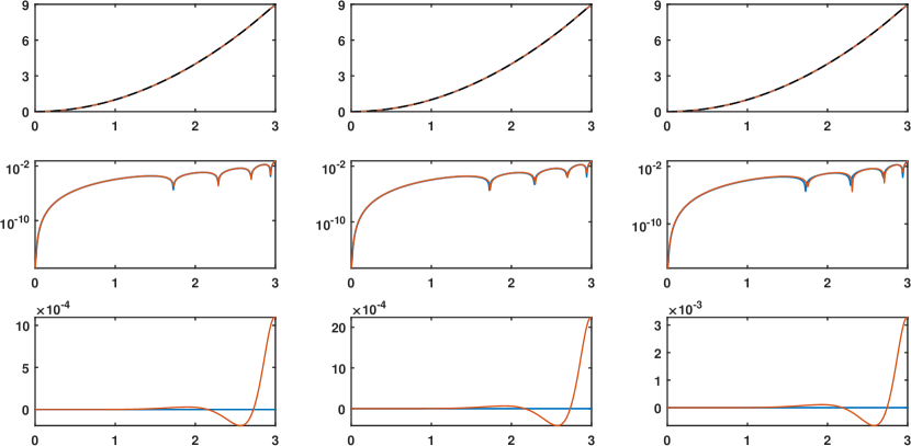
Refer to caption
Figure 13: Modified wavenumber, and real and imaginary components of the spectral error for left-biased 𝓞ML,MRML,MR(4)\boldsymbol{\mathcal{O}}^{M_{L},M_{R}}_{M_{L},M_{R}}(4) approximating the second derivative. N¯=7\bar{N}=7, γ(η)=1\gamma(\eta)=1 for η[0,3]\eta\in[0,3], and γ(η)=0\gamma(\eta)=0 otherwise.
Refer to caption
Figure 14: Modified wavenumber, and real and imaginary components of the spectral error for left-biased 𝓞ML,MRML,MR(4)\boldsymbol{\mathcal{O}}^{M_{L},M_{R}}_{M_{L},M_{R}}(4) approximating the first derivative. N¯=7\bar{N}=7, γ(η)=1\gamma(\eta)=1 for η[0,3]\eta\in[0,3], and γ(η)=0\gamma(\eta)=0 otherwise.

Fig.13 and Fig.14 compare modified wavenumbers of different implicit left-biased schemes (ML=4,5,6M_{L}=4,5,6, red) with the implicit central scheme (M=3M=3, blue) of equal true stencil size (N¯=2M+1=7\bar{N}=2M+1=7) for second and first derivatives respectively. Numerical values of the optimal coefficients are tabulated in Table 3 and 4.

From the middle row of Fig.13, we observe that the variation of the real component [e(η)]\Re[e(\eta)] (shown in log scale) for biased schemes (red) is very close to that of the central scheme of same stencil size (blue).

In case of central scheme (blue), the imaginary component [e(η)]\Im[e(\eta)] for even derivatives is zero, which is seen in the last row of Fig.13 (see Lemma 2 and Fig.2). And as expected, the imaginary component [e(η)]\Im[e(\eta)] for biased schemes (red) which approximate even derivatives is not zero. This is due to the fact that Lemma 2 does not hold for biased schemes as constraint Eq.(73) imposes asymmetry on optimal coefficients. For fixed true stencil size, as MLM_{L} increases, MR=N¯(ML+1)M_{R}=\bar{N}-(M_{L}+1) decreases and schemes become more biased. It can be observed from the last row of Fig.13 that the imaginary component [e(η)]\Im[e(\eta)] increases with increase in biasedness of the scheme.

Similarly, the middle row of Fig.14 shows that unlike the central scheme (blue), real component [e(η)]\Re[e(\eta)] for biased schemes (red) which approximate odd derivatives is not zero, and its magnitude increases with the increase in biasedness of the scheme. However, the variation of imaginary component [e(η)]\Im[e(\eta)] (shown in log scale) for biased schemes (red) is very close to that of the central scheme (blue).

While solving PDEs numerically, we use a central scheme of stencil size (2M+12M+1) at (Np2MN_{p}-2M) points within the domain and biased schemes at MM points adjacent to each one of left and right boundaries of the domain. Therefore, (Np2MN_{p}-2M) middle rows of 𝐀d\mathbf{A}_{d} and 𝐁d\mathbf{B}_{d} defined in Eq.(37) contain same central scheme coefficients, last MM rows contain left-biased scheme coefficients and first MM rows contain complementary right-biased scheme coefficients. Then 𝐀d𝚽\mathbf{A}_{d}^{\mathbf{\Phi}} and 𝐁d𝚽\mathbf{B}_{d}^{\mathbf{\Phi}} for such non-periodic discretization can be constructed similar to Eq.(38). Semi-discrete stability discussed in Section 3.1 is not valid for biased approximations since coefficients do not satisfy properties described in Lemma 2 and 3. However, Eq.(41) and Eq.(42) hold true for non-periodic discretization. Therefore, fully discretized stability analysis presented in Section 3.2.2 is valid for this case.

Special cases discussed in this section are a few examples which demonstrate how to derive optimal finite difference schemes with desired structure by imposing suitable constraints on coefficients. Since all constraints are linear, one can impose any number and combination of constraints Eq.(61), Eq.(66) and Eq.(72) to obtain desirable schemes. For example, we can impose constraints in Eq.(66) and Eq.(72) simultaneously and solve the resulting optimization problem to derive biased schemes which are spatially explicit. However, to ensure the invertibility of the matrix 𝐏\mathbf{P}, such as in Eq.(74), duplicate constraints should be removed while constructing the KKT condition.

5 Numerical Results

In this section we use optimized schemes derived in preceding sections to solve some PDEs numerically and compare the results with the standard schemes. In particular, we benchmark our optimized schemes against following:

  1. (a)

    Standard schemes of same order

  2. (b)

    Standard schemes of same stencil size

Initial condition for solving PDEs is taken to be the superposition of multiple sinusoidal waves with wavenumbers kk, given by Eq.(75). A(k)A(k) is amplitude of the wave corresponding to wavenumber kk, and ϕk[0,2π]\phi_{k}\in[0,2\pi] is the corresponding phase initialized randomly. We use the same initial condition for solving different PDEs in sections to follow.

f0(x):=f(x,t=0)=kA(k)sin(kx+ϕk).\displaystyle f_{0}(x):=f(x,t=0)=\sum_{k}A(k)\sin(kx+\phi_{k}). (75)

5.1 Advection-diffusion equation

Consider the following simplified version of Eq.(36), where coefficients of only first two spatial derivatives are non-zero.

ft=β1fx+β22fx2.\displaystyle\frac{\partial f}{\partial t}=\beta_{1}\frac{\partial f}{\partial x}+\beta_{2}\frac{\partial^{2}f}{\partial x^{2}}. (76)

To satisfy Eq.(46), we have diffusivity β2>0\beta_{2}>0. Analytical solution for Eq.(76) is known and given by

ft(x)a:=f(x,t>0)a=kexp(β2k2t)A(k)sin(k(x+β1t)+ϕk),\displaystyle f_{t}(x)_{a}:=f(x,t>0)_{a}=\sum_{k}\exp({-\beta_{2}k^{2}t})A(k)\sin(k(x+\beta_{1}t)+\phi_{k}), (77)

where subscript aa stands for the analytical solution. In this case, amplitude decays with time due to non-zero β2\beta_{2} and phase also changes due to non-zero β1\beta_{1}.

We used CFL number to express Δt\Delta t and Δx\Delta x as a normalized quantity. Similarly, we define normalized time with respect to dthd^{th} derivative as td:=|βd|tkmaxdt^{\ast}_{d}:=|\beta_{d}|tk_{\max}^{d}, where kmaxk_{\max} is the largest wavenumber present in the initial condition Eq.(75). Eq.(76) is solved using various optimized and standard spatial finite difference schemes. For a fixed diffusive CFL (r2r_{2}), we have used matching order explicit Runge-Kutta (ERK) schemes for the temporal discretization. For example, for spatial schemes which are 4th4^{\text{th}} and 10th10^{\text{th}} order accurate, we have used 2nd2^{\text{nd}} and 5th5^{\text{th}} order ERK for the temporal discretization respectively.

The spectral energy at wavenumber kk at time tt is defined to be |f^t(k)|2|\hat{f}_{t}(k)|^{2}, where f^t(k)\hat{f}_{t}(k) is the discrete Fourier coefficient corresponding to wavenumber kk at time tt. To assess the dissipative numerical errors at different wavenumbers, we plot normalized error in spectral energy of the numerical solution with respect to the analytical solution in Fig.15. These results are obtained for diffusive CFL number r2=0.01r_{2}=0.01 at t225t^{\ast}_{2}\approx 25.

Error is small for the standard scheme, 𝓢11(4)\boldsymbol{\mathcal{S}}^{1}_{1}(4) (cyan), in low wavenumber region. However, error grows drastically as wavenumber increases. The standard pentadiagonal scheme, 𝓢23(10)\boldsymbol{\mathcal{S}}^{3}_{2}(10) (black), shows better spectral accuracy than 𝓢11(4)\boldsymbol{\mathcal{S}}^{1}_{1}(4) across all wavenumbers. Although, error in high wavenumber region is significantly large for 𝓢23(10)\boldsymbol{\mathcal{S}}^{3}_{2}(10) as well.

The optimized pentadiagonal scheme, 𝓞23(4)\boldsymbol{\mathcal{O}}^{3}_{2}(4) (red), shows better accuracy than 𝓢11(4)\boldsymbol{\mathcal{S}}^{1}_{1}(4) (cyan) at all wavenumbers. 𝓞23(4)\boldsymbol{\mathcal{O}}^{3}_{2}(4) has larger error than 𝓢23(10)\boldsymbol{\mathcal{S}}^{3}_{2}(10) (black) at lower wavenumbers. But at higher wavenumbers, the 4th4^{\text{th}} order accurate 𝓞23(4)\boldsymbol{\mathcal{O}}^{3}_{2}(4) demonstrates much better accuracy than 10th10^{\text{th}} order accurate 𝓢23(10)\boldsymbol{\mathcal{S}}^{3}_{2}(10).

Overall, 𝓞33(4)\boldsymbol{\mathcal{O}}^{3}_{3}(4) (blue) shows better accuracy than pentadiagonal 𝓞23(4)\boldsymbol{\mathcal{O}}^{3}_{2}(4) (red), which is in accordance with Remark 1.

Both standard schemes, 𝓢11(4)\boldsymbol{\mathcal{S}}^{1}_{1}(4) (cyan) and 𝓢23(10)\boldsymbol{\mathcal{S}}^{3}_{2}(10) (black), demonstrate steep variation of error as wavenumber is increased. On the other hand, optimized schemes 𝓞23(4)\boldsymbol{\mathcal{O}}^{3}_{2}(4) (red) and 𝓞33(4)\boldsymbol{\mathcal{O}}^{3}_{3}(4) (blue) show relatively slower variation of error with increasing wavenumber. Again, this behavior is expected due to equally weighted wavenumbers (γ(η)=1\gamma(\eta)=1) in the optimization.

Refer to caption
Figure 15: Diffusion error for advection-diffusion equation. Blue – 𝓞33(4)\boldsymbol{\mathcal{O}}^{3}_{3}(4); red – 𝓞23(4)\boldsymbol{\mathcal{O}}^{3}_{2}(4); black – 𝓢23(10)\boldsymbol{\mathcal{S}}^{3}_{2}(10); cyan – 𝓢11(4)\boldsymbol{\mathcal{S}}^{1}_{1}(4). r1r2=0.01r_{1}\approx r_{2}=0.01, t225t^{\ast}_{2}\approx 25, A(k)=1A(k)=1, γ(η)=1\gamma(\eta)=1 for η[0,3]\eta\in[0,3], and γ(η)=0\gamma(\eta)=0 otherwise.

While Fig.15 shows numerical dissipation error, the dispersion error is shown in Fig.16. Dispersion error is quantified by calculation of numerical speed, cn(k):=arg[f^t(k)/f^0(k)]/ktc_{n}(k):=\arg[\hat{f}_{t}(k)/\hat{f}_{0}(k)]/kt. Analytical speed is ca:=β1c_{a}:=\beta_{1} for all wavenumbers. Normalized numerical speed, c(k):=cn(k)/cac^{\ast}(k):=c_{n}(k)/c_{a}, is unity when there is no dispersion error. Normalized numerical speed and error for different schemes are shown in Fig.16.

Observations made for Fig.15 are consistent with Fig.16 as well. From Fig.16, it is evident that normalized numerical speed for standard schemes, 𝓢11(4)\boldsymbol{\mathcal{S}}^{1}_{1}(4) (cyan) and 𝓢23(10)\boldsymbol{\mathcal{S}}^{3}_{2}(10) (black), deviates from unity at lower wavenumbers leading to large dispersion error at higher wavenumbers. The normalized numerical speed for optimized schemes 𝓞23(4)\boldsymbol{\mathcal{O}}^{3}_{2}(4) (red) and 𝓞33(4)\boldsymbol{\mathcal{O}}^{3}_{3}(4) (blue), is close to unity even at higher wavenumbers. As in the case of dissipative error, here also we observe that the standard schemes show steep variation of dispersion error, while the optimized schemes are relatively slower in variation.
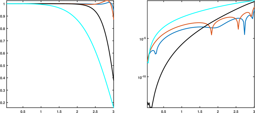
Refer to caption
Figure 16: Dispersion error for advection-diffusion equation. Blue – 𝓞33(4)\boldsymbol{\mathcal{O}}^{3}_{3}(4); red – 𝓞23(4)\boldsymbol{\mathcal{O}}^{3}_{2}(4); black – 𝓢23(10)\boldsymbol{\mathcal{S}}^{3}_{2}(10); cyan – 𝓢11(4)\boldsymbol{\mathcal{S}}^{1}_{1}(4). r1r2=0.01r_{1}\approx r_{2}=0.01, t225t^{\ast}_{2}\approx 25, A(k)=1A(k)=1, γ(η)=1\gamma(\eta)=1 for η[0,3]\eta\in[0,3], and γ(η)=0\gamma(\eta)=0 otherwise.

5.2 Non-linear advection-diffusion equation

Now let us consider non-linear advection-diffusion equation which is also known as Burgers’ equation and widely studied in various areas of applied mathematics.

ft=ffx+β22fx2.\displaystyle\frac{\partial f}{\partial t}=-f\frac{\partial f}{\partial x}+\beta_{2}\frac{\partial^{2}f}{\partial x^{2}}. (78)

Because of the non-linear term, different Fourier modes interact with each other and produce new wavenumbers in the solution. Therefore, to ensure that all wavenumbers are well resolved, we performed grid convergence study and observed that space-averaged energy (K:=i=1Npfi2(x,t)/NpK:=\sum_{i=1}^{N_{p}}f_{i}^{2}(x,t)/N_{p}) becomes independent of the number of grid points in the domain at Np=256N_{p}=256.

Numerical solution of Eq.(78) is obtained in a periodic domain x[0,2π]x\in[0,2\pi] with initial condition given by Eq.(75), where A(k)=k1/2A(k)=k^{-1/2}. The negative exponent ensures that higher wavenumbers have sufficient energy content without being unstable. For this particular PDE, we define timescale as t=K/ϵt=K/\epsilon, where ϵ\epsilon is space averaged energy dissipation rate (ϵ:=i=1Np(fi(x,t)/x)2/Np\epsilon:=\sum_{i=1}^{N_{p}}(\partial f_{i}(x,t)/\partial x)^{2}/N_{p}). Then time is expressed as a normalized quantity t:=t/t0t^{\ast}:=t/t_{0} where t0=K0/ϵ0t_{0}=K_{0}/\epsilon_{0} is the initial timescale.

The analytical solution of Eq.(78) is obtained by applying Cole-Hopf transformation as follows [15, 16]. First, let us define the transformation

f=2β21ϕϕx.\displaystyle f=-2\beta_{2}\frac{1}{\phi}\frac{\partial\phi}{\partial x}.

With this substitution, Eq.(78) becomes diffusion equation and the analytical solution for f(x,t)f(x,t) is given by

f(x,t)=xytϕ(y,0)exp((xy)24β2t)𝑑yϕ(y,0)exp((xy)24β2t)𝑑y,\displaystyle f(x,t)=\frac{\int_{-\infty}^{\infty}\frac{x-y}{t}\phi(y,0)\exp\Big(\frac{(x-y)^{2}}{4\beta_{2}t}\Big)dy}{\int_{-\infty}^{\infty}\phi(y,0)\exp\Big(\frac{(x-y)^{2}}{4\beta_{2}t}\Big)dy}, (79)

where initial ϕ(y,0)\phi(y,0) is obtained using

ϕ(y,0)=exp(0yf(z,0)2β2dz).\displaystyle\phi(y,0)=\exp\Big(-\int_{0}^{y}\frac{f(z,0)}{2\beta_{2}}dz\Big).

Eq.(79) is the exact solution for non-linear advection-diffusion equation. However, integrals involved are computed numerically.

Fig.17 shows the spectral energy content normalized with initial energy for different wavenumbers. All numerical results for this PDE are obtained for β2=0.04\beta_{2}=0.04, r2=0.01r_{2}=0.01 at t104t^{\ast}\approx 104. It can be clearly seen that the spectral energy content for standard schemes 𝓢11(4)\boldsymbol{\mathcal{S}}^{1}_{1}(4) (cyan) and 𝓢23(10)\boldsymbol{\mathcal{S}}^{3}_{2}(10) (black solid) deviates from analytical solution (black dashed) at high wavenumbers. In the same wavenumber region, the optimized schemes 𝓞23(4)\boldsymbol{\mathcal{O}}^{3}_{2}(4) (red) and 𝓞33(4)\boldsymbol{\mathcal{O}}^{3}_{3}(4) (blue) are relatively closer to the analytical solution.
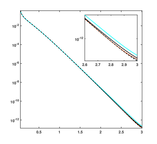
Refer to caption
Figure 17: Spectral energy content for non-linear advection-diffusion equation normalized with initial energy. Blue – 𝓞33(4)\boldsymbol{\mathcal{O}}^{3}_{3}(4); red – 𝓞23(4)\boldsymbol{\mathcal{O}}^{3}_{2}(4); black – 𝓢23(10)\boldsymbol{\mathcal{S}}^{3}_{2}(10); cyan – 𝓢11(4)\boldsymbol{\mathcal{S}}^{1}_{1}(4); black dashed – analytical solution. β2=0.04\beta_{2}=0.04, r2=0.01r_{2}=0.01, A(k)=k1/2A(k)=k^{-1/2}, t104t^{\ast}\approx 104, kmax=121k_{\max}=121, γ(η)=1\gamma(\eta)=1 for η[0,3]\eta\in[0,3], and γ(η)=0\gamma(\eta)=0 otherwise.

Similar to Fig.15, we show the normalized error in spectral energy for the non-linear advection-diffusion equation in Fig.18. Due to the interaction of Fourier modes with each other, in general, we do not expect the spectral behavior of different schemes for non-linear PDE to be in exact agreement with the behavior observed for the linear case. Unlike the linear case (Fig.15), Fig.18 shows that the optimized schemes 𝓞23(4)\boldsymbol{\mathcal{O}}^{3}_{2}(4) (red) and 𝓞33(4)\boldsymbol{\mathcal{O}}^{3}_{3}(4) (blue) have better accuracy than 𝓢23(10)\boldsymbol{\mathcal{S}}^{3}_{2}(10) (black) in both low and high wavenumber region. Overall, 𝓢11(4)\boldsymbol{\mathcal{S}}^{1}_{1}(4) (cyan) has the largest error. The error for 𝓞33(4)\boldsymbol{\mathcal{O}}^{3}_{3}(4) is somewhat comparable to the pentadiagonal 𝓞23(4)\boldsymbol{\mathcal{O}}^{3}_{2}(4).

Refer to caption
Figure 18: Diffusion error for non-linear advection-diffusion equation. Blue – 𝓞33(4)\boldsymbol{\mathcal{O}}^{3}_{3}(4); red – 𝓞23(4)\boldsymbol{\mathcal{O}}^{3}_{2}(4); black – 𝓢23(10)\boldsymbol{\mathcal{S}}^{3}_{2}(10); cyan – 𝓢11(4)\boldsymbol{\mathcal{S}}^{1}_{1}(4). β2=0.04\beta_{2}=0.04, r2=0.01r_{2}=0.01, A(k)=k1/2A(k)=k^{-1/2}, t104t^{\ast}\approx 104, kmax=121k_{\max}=121, γ(η)=1\gamma(\eta)=1 for η[0,3]\eta\in[0,3], and γ(η)=0\gamma(\eta)=0 otherwise.

Because of the non-linearity, there is no well-defined analytical speed in this case and therefore, the notion of numerical speed can not be used to quantify the dispersion error. However, we can calculate and compare the argument of Fourier coefficients, θk^:=arg[f^t(k)]\hat{\theta_{k}}:=\arg[\hat{f}_{t}(k)], for different wavenumbers. Normalized error in θk^\hat{\theta_{k}} is shown in Fig.19. Clearly, the optimized schemes 𝓞23(4)\boldsymbol{\mathcal{O}}^{3}_{2}(4) (red) and 𝓞33(4)\boldsymbol{\mathcal{O}}^{3}_{3}(4) (blue) have smaller phase error than the standard schemes 𝓢11(4)\boldsymbol{\mathcal{S}}^{1}_{1}(4) (cyan) and 𝓢23(10)\boldsymbol{\mathcal{S}}^{3}_{2}(10) (black) across all wavenumbers. Whereas, in the linear case (Fig.16) 𝓢23(10)\boldsymbol{\mathcal{S}}^{3}_{2}(10) demonstrates better accuracy than the optimized schemes in the low wavenumber region. Also, 𝓞33(4)\boldsymbol{\mathcal{O}}^{3}_{3}(4) shows better accuracy than the pentadiagonal 𝓞23(4)\boldsymbol{\mathcal{O}}^{3}_{2}(4) in Fig.19.

Refer to caption
Figure 19: Phase error for non-linear advection-diffusion equation. Blue – 𝓞33(4)\boldsymbol{\mathcal{O}}^{3}_{3}(4); red – 𝓞23(4)\boldsymbol{\mathcal{O}}^{3}_{2}(4); black – 𝓢23(10)\boldsymbol{\mathcal{S}}^{3}_{2}(10); cyan – 𝓢11(4)\boldsymbol{\mathcal{S}}^{1}_{1}(4). β2=0.04\beta_{2}=0.04, r2=0.01r_{2}=0.01, A(k)=k1/2A(k)=k^{-1/2}, t104t^{\ast}\approx 104, kmax=121k_{\max}=121, γ(η)=1\gamma(\eta)=1 for η[0,3]\eta\in[0,3], and γ(η)=0\gamma(\eta)=0 otherwise.

Fig.18 and Fig.19 independently quantify the errors in |f^t(k)||\hat{f}_{t}(k)| and θk^\hat{\theta_{k}}. Fig.20 accounts for |f^t(k)f^t(k)a||\hat{f}_{t}(k)-\hat{f}_{t}(k)_{a}|, which quantifies the combined effect of error in |f^t(k)||\hat{f}_{t}(k)| and θk^\hat{\theta_{k}} in a single plot. When we look at the combined error in the non-linear case, it is observed from Fig.20 that the optimized schemes 𝓞23(4)\boldsymbol{\mathcal{O}}^{3}_{2}(4) (red) and 𝓞33(4)\boldsymbol{\mathcal{O}}^{3}_{3}(4) (blue) have better accuracy than the standard schemes 𝓢11(4)\boldsymbol{\mathcal{S}}^{1}_{1}(4) (cyan) and 𝓢23(10)\boldsymbol{\mathcal{S}}^{3}_{2}(10) (black) at all wavenumbers. Moreover, 𝓞33(4)\boldsymbol{\mathcal{O}}^{3}_{3}(4) demonstrates better accuracy than the pentadiagonal 𝓞23(4)\boldsymbol{\mathcal{O}}^{3}_{2}(4) and hence reinforcing Remark 1. Thus, for solving practical physical problems which are governed by non-linear PDEs, optimized schemes seem to provide much better spectral resolution than the non-optimized standard schemes.
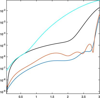
Refer to caption
Figure 20: Amplitude error for non-linear advection-diffusion equation. Blue – 𝓞33(4)\boldsymbol{\mathcal{O}}^{3}_{3}(4); red – 𝓞23(4)\boldsymbol{\mathcal{O}}^{3}_{2}(4); black – 𝓢23(10)\boldsymbol{\mathcal{S}}^{3}_{2}(10); cyan – 𝓢11(4)\boldsymbol{\mathcal{S}}^{1}_{1}(4). β2=0.04\beta_{2}=0.04, r2=0.01r_{2}=0.01, A(k)=k1/2A(k)=k^{-1/2}, t104t^{\ast}\approx 104, kmax=121k_{\max}=121, γ(η)=1\gamma(\eta)=1 for η[0,3]\eta\in[0,3], and γ(η)=0\gamma(\eta)=0 otherwise.

6 Conclusions

Central compact standard finite differences are derived using the popular pentadiagonal 7 point stencil formulation to maximize formal order of accuracy of the approximation. In this paper, we presented a generalized unified framework to derive central compact optimal schemes with equal LHS and RHS stencil sizes. The optimal coefficients are determined analytically by solving an optimization problem. The cost function, defined to be the 2\mathcal{L}_{2} norm of spectral error, is minimized subject to linear equality constraints in coefficients. We have shown that for a given order of accuracy, we can increase the stencil size and hence the number of degrees of freedom in the optimization to achieve better spectral resolution. The freedom of selecting weighting function (γ(η)\gamma(\eta)) allows us to achieve better resolution of the wavenumbers which are important to the physics of problem by giving them more weightage in the optimization problem. We have also presented an analytical justification for the symmetry/skew-symmetry of optimal coefficients resulting in purely real or imaginary error which depends on order of the derivative being approximated.

We have shown that special cases namely, central schemes with unequal LHS and RHS stencil sizes (e.g. pentadiagonal), explicit, and biased schemes can be derived by imposing additional linear constraints in the optimization problem. Using these three special cases as building blocks, an optimal scheme with any desired structure can be derived as all constraints are linear and therefore, they can be imposed in any number and combination.

We have also presented a rigorous stability analysis for a generalized implicit RK scheme. We showed that by increasing the stencil size the spectral resolution can be improved, but simultaneously it results in reduced stability region in r1r2r_{1}-r_{2} space.

Finally, we presented numerical results for optimized schemes to benchmark them against the standard schemes of the same accuracy order, and the same stencil size. The optimized schemes show better accuracy than the standard scheme of the same stencil size with larger formal order of accuracy in the high wavenumber region. The better resolution in high wavenumber region is achieved at the expense of relatively larger error at the lower wavenumbers, because γ(η)=1\gamma(\eta)=1 used in simulations weights all wavenumbers equally. However, in the case of non-linear PDE, we observed that the optimized schemes show overall better accuracy than the standard schemes across the wavenumber spectrum.

The observation, compact schemes with equal LHS and RHS stencil sizes demonstrate better performance than those with unequal stencil sizes, has been reinforced through numerical simulations. However, we recognize that the usage of schemes with equal LHS and RHS stencil sizes e.g., 𝓞33()\boldsymbol{\mathcal{O}}^{3}_{3}(\cdot), might prove to be impractical for large simulations as the computation cost for 𝓞33()\boldsymbol{\mathcal{O}}^{3}_{3}(\cdot) can be substantially higher than that of pentadiagonal 𝓞23()\boldsymbol{\mathcal{O}}^{3}_{2}(\cdot). A different study will be performed in the future to assess the tradeoff between the accuracy we gain and the computation cost we incur due to usage of schemes such as 𝓞33()\boldsymbol{\mathcal{O}}^{3}_{3}(\cdot). To reduce the computational cost, we intend to develop the present framework further to derive prefactored optimized schemes such as presented in [5, 6, 8].

Empirical observations show that KKT matrix used in determining optimal coefficients of implicit schemes suffer from rank deficiency at certain stencil size (MM). However, explicit schemes are unaffected by this problem. This issue, perhaps, hints at the fundamental limitation of implicit schemes to scale up beyond certain stencil size, and it will be investigated in our future studies.

Although our framework allows us to derive biased schemes, for the brevity of discussion we have restricted numerical results presented in this work on periodic domains. Also, implementation of boundary conditions without compromising the accuracy of numerical solution is an important area of research and will be addressed in our future work.

Appendix A Invariance of grid point location

Lemma 4.

Optimal implicit central finite-difference approximation is invariant of the grid point location in the domain.

Proof.

Let the coefficients for the dthd^{\text{th}} derivative at the ithi^{\text{th}} grid point corresponding to Eq.(2) be parameterized by 𝐚i,d{\mathbf{a}}_{i,d} and 𝐛i,d{\mathbf{b}}_{i,d}, and 𝐀d\mathbf{A}_{d} and 𝐁d\mathbf{B}_{d} be the vertical stacking of 𝐚i,dT\mathbf{a}^{T}_{i,d} and 𝐛i,dT\mathbf{b}^{T}_{i,d} respectively, i.e.

𝐀d:=[𝐚1,dT𝐚Np,dT],𝐁d:=[𝐛1,dT𝐛Np,dT].\displaystyle\mathbf{A}_{d}:=\begin{bmatrix}{\mathbf{a}}_{1,d}^{T}\\ \vdots\\ {\mathbf{a}}_{N_{p},d}^{T}\end{bmatrix},\;\mathbf{B}_{d}:=\begin{bmatrix}{\mathbf{b}}_{1,d}^{T}\\ \vdots\\ {\mathbf{b}}_{N_{p},d}^{T}\end{bmatrix}.

The order accuracy constraint, for every 𝐚i,d,𝐛i,d\mathbf{a}_{i,d},\mathbf{b}_{i,d} pair, can be compactly written as

[𝐀d𝐁d][𝐗d𝐘d]=𝟎Np×(d+p+1).\displaystyle\begin{bmatrix}\mathbf{A}_{d}&\mathbf{B}_{d}\end{bmatrix}\begin{bmatrix}\mathbf{X}_{d}\\ -\mathbf{Y}_{d}\end{bmatrix}=\mathbf{0}_{N_{p}\times(d+p+1)}.

The cost function over NpN_{p} grid points in the entire domain is

i=1Np(𝐚i,d𝐛i,d)T𝐐d(𝐚i,d𝐛i,d).\displaystyle\sum_{i=1}^{N_{p}}\begin{pmatrix}\mathbf{a}_{i,d}\\ \mathbf{b}_{i,d}\end{pmatrix}^{T}\mathbf{Q}_{d}\begin{pmatrix}\mathbf{a}_{i,d}\\ \mathbf{b}_{i,d}\end{pmatrix}.

Optimization of the spectral error is separable for different derivatives, and can be formulated as following from Eq.(20)

mini=1Np𝐚i,d,𝐛i,d(𝐚i,d𝐛i,d)T𝐐d(𝐚i,d𝐛i,d), subject to [𝐀d𝐁d][𝐗d𝐘d]=𝟎Np×(d+p+1),𝐁d𝜹N(M+1)=𝟏N×1,}\left.\begin{aligned} &\min_{\mathbf{a}_{i,d},\mathbf{b}_{i,d}}\sum_{i=1}^{N_{p}}\begin{pmatrix}\mathbf{a}_{i,d}\\ \mathbf{b}_{i,d}\end{pmatrix}^{T}\mathbf{Q}_{d}\begin{pmatrix}\mathbf{a}_{i,d}\\ \mathbf{b}_{i,d}\end{pmatrix},\\ &\text{ subject to }\\ &\begin{bmatrix}\mathbf{A}_{d}&\mathbf{B}_{d}\end{bmatrix}\begin{bmatrix}\mathbf{X}_{d}\\ -\mathbf{Y}_{d}\end{bmatrix}=\mathbf{0}_{N_{p}\times(d+p+1)},\\ &\mathbf{B}_{d}\boldsymbol{\delta}_{N}(M+1)=\mathbf{1}_{N\times 1},\end{aligned}\;\;\right\} (80)

for d=1,,Dd=1,\cdots,D. Let us define vector,

𝐯d:=(𝐚1,d𝐛1,d𝐚Np,d𝐛Np,d).\displaystyle\mathbf{v}_{d}:=\begin{pmatrix}\mathbf{a}_{1,d}\\ \mathbf{b}_{1,d}\\ \vdots\\ \mathbf{a}_{N_{p},d}\\ \mathbf{b}_{N_{p},d}\end{pmatrix}.

The optimization in Eq.(80), can be written in terms of 𝐯d\mathbf{v}_{d} as

min𝐯d𝐯dT(𝐈Np𝐐d)𝐯d, subject to(𝐈Np[𝐗dT𝐘dT𝟎1×N𝜹NT(M+1)])𝐯d=𝟏Np×1𝜹n(n),\displaystyle\min_{\mathbf{v}_{d}}\mathbf{v}_{d}^{T}\left(\mathbf{I}_{N_{p}}\otimes\mathbf{Q}_{d}\right)\mathbf{v}_{d},\text{ subject to}\left(\mathbf{I}_{N_{p}}\otimes\begin{bmatrix}\mathbf{X}_{d}^{T}&-\mathbf{Y}_{d}^{T}\\ \mathbf{0}_{1\times N}&\boldsymbol{\delta}_{N}^{T}(M+1)\end{bmatrix}\right)\mathbf{v}_{d}=\mathbf{1}_{N_{p}\times 1}\otimes\boldsymbol{\delta}_{n}(n),

for n=(d+p+2)n=(d+p+2). Then the analytical solution given by

(𝐯d𝚲d)=[𝐈Np𝐐d𝐈Np(𝐗dT𝐘dT𝟎1×N𝜹NT(M+1))T𝐈Np(𝐗dT𝐘dT𝟎1×N𝜹NT(M+1))𝐈Np𝟎(d+p+2)×(d+p+2)]1[𝟏Np×1𝟎2N×1𝟏Np×1𝜹n(n)].\displaystyle\begin{pmatrix}\mathbf{v}_{d}^{\ast}\\ \boldsymbol{\Lambda}_{d}^{\ast}\end{pmatrix}=\left[\begin{array}[]{cc}\mathbf{I}_{N_{p}}\otimes\mathbf{Q}_{d}&\mathbf{I}_{N_{p}}\otimes\left(\begin{array}[]{cc}\mathbf{X}_{d}^{T}&-\mathbf{Y}_{d}^{T}\\ \mathbf{0}_{1\times N}&\boldsymbol{\delta}_{N}^{T}(M+1)\end{array}\right)^{T}\\ \mathbf{I}_{N_{p}}\otimes\left(\begin{array}[]{cc}\mathbf{X}_{d}^{T}&-\mathbf{Y}_{d}^{T}\\ \mathbf{0}_{1\times N}&\boldsymbol{\delta}_{N}^{T}(M+1)\end{array}\right)&\mathbf{I}_{N_{p}}\otimes\mathbf{0}_{(d+p+2)\times(d+p+2)}\end{array}\right]^{-1}\begin{bmatrix}\mathbf{1}_{N_{p}\times 1}\otimes\mathbf{0}_{2N\times 1}\\ \mathbf{1}_{N_{p}\times 1}\otimes\boldsymbol{\delta}_{n}(n)\end{bmatrix}.

Inverse of a partitioned matrix is given by

[𝐀𝐁𝐂𝐃]1=[𝐀1+𝐀1𝐁(𝐃𝐂𝐀1𝐁)1𝐂𝐀1𝐀1𝐁(𝐃𝐂𝐀1𝐁)1(𝐃𝐂𝐀1𝐁)1𝐂𝐀1(𝐃𝐂𝐀1𝐁)1].\displaystyle\begin{bmatrix}\mathbf{A}&\mathbf{B}\\ \mathbf{C}&\mathbf{D}\end{bmatrix}^{-1}={\begin{bmatrix}\mathbf{A}^{-1}+\mathbf{A}^{-1}\mathbf{B}(\mathbf{D}-\mathbf{CA}^{-1}\mathbf{B})^{-1}\mathbf{CA}^{-1}&-\mathbf{A}^{-1}\mathbf{B}(\mathbf{D}-\mathbf{CA}^{-1}\mathbf{B})^{-1}\\ -(\mathbf{D}-\mathbf{CA}^{-1}\mathbf{B})^{-1}\mathbf{CA}^{-1}&(\mathbf{D}-\mathbf{CA}^{-1}\mathbf{B})^{-1}\end{bmatrix}}. (81)

Let,

[𝐐d(𝐗dT𝐘dT𝟎1×N𝜹NT(M+1))T(𝐗dT𝐘dT𝟎1×N𝜹NT(M+1))𝟎(d+p+2)×(d+p+2)]1:=[𝐌1𝐌2𝐌3𝐌4],\displaystyle\left[\begin{array}[]{cc}\mathbf{Q}_{d}&\left(\begin{array}[]{cc}\mathbf{X}_{d}^{T}&-\mathbf{Y}_{d}^{T}\\ \mathbf{0}_{1\times N}&\boldsymbol{\delta}_{N}^{T}(M+1)\end{array}\right)^{T}\\ \left(\begin{array}[]{cc}\mathbf{X}_{d}^{T}&-\mathbf{Y}_{d}^{T}\\ \mathbf{0}_{1\times N}&\boldsymbol{\delta}_{N}^{T}(M+1)\end{array}\right)&\mathbf{0}_{(d+p+2)\times(d+p+2)}\end{array}\right]^{-1}:=\begin{bmatrix}\mathbf{M}_{1}&\mathbf{M}_{2}\\ \mathbf{M}_{3}&\mathbf{M}_{4}\end{bmatrix},

where 𝐌i\mathbf{M}_{i} are obtained using Eq.(81). Using the identity

(𝐀𝐁)(𝐂𝐃)=𝐀𝐂𝐁𝐃,\displaystyle(\mathbf{A}\otimes\mathbf{B})(\mathbf{C}\otimes\mathbf{D})=\mathbf{AC}\otimes\mathbf{BD},

and Eq.(81), we get

[𝐈Np𝐐d𝐈Np(𝐗dT𝐘dT𝟎1×N𝜹NT(M+1))T𝐈Np(𝐗dT𝐘dT𝟎1×N𝜹NT(M+1))𝐈Np𝟎(d+p+2)×(d+p+2)]1=[𝐈Np𝐌1𝐈Np𝐌2𝐈Np𝐌3𝐈Np𝐌4].\displaystyle\left[\begin{array}[]{cc}\mathbf{I}_{N_{p}}\otimes\mathbf{Q}_{d}&\mathbf{I}_{N_{p}}\otimes\left(\begin{array}[]{cc}\mathbf{X}_{d}^{T}&-\mathbf{Y}_{d}^{T}\\ \mathbf{0}_{1\times N}&\boldsymbol{\delta}_{N}^{T}(M+1)\end{array}\right)^{T}\\ \mathbf{I}_{N_{p}}\otimes\left(\begin{array}[]{cc}\mathbf{X}_{d}^{T}&-\mathbf{Y}_{d}^{T}\\ \mathbf{0}_{1\times N}&\boldsymbol{\delta}_{N}^{T}(M+1)\end{array}\right)&\mathbf{I}_{N_{p}}\otimes\mathbf{0}_{(d+p+2)\times(d+p+2)}\end{array}\right]^{-1}=\begin{bmatrix}\mathbf{I}_{N_{p}}\otimes\mathbf{M}_{1}&\mathbf{I}_{N_{p}}\otimes\mathbf{M}_{2}\\ \mathbf{I}_{N_{p}}\otimes\mathbf{M}_{3}&\mathbf{I}_{N_{p}}\otimes\mathbf{M}_{4}\end{bmatrix}.

Therefore, the optimal solution

(𝐯d𝚲d)\displaystyle\begin{pmatrix}\mathbf{v}_{d}^{\ast}\\ \boldsymbol{\Lambda}_{d}^{\ast}\end{pmatrix} =[(𝐈Np𝐌1)(𝟏Np×1𝟎2N×1)+(𝐈Np𝐌2)(𝟏Np×1𝜹n(n))(𝐈Np𝐌3)(𝟏Np×1𝟎2N×1)+(𝐈Np𝐌4)(𝟏Np×1𝜹n(n))],\displaystyle=\begin{bmatrix}\left(\mathbf{I}_{N_{p}}\otimes\mathbf{M}_{1}\right)\left(\mathbf{1}_{N_{p}\times 1}\otimes\mathbf{0}_{2N\times 1}\right)+\left(\mathbf{I}_{N_{p}}\otimes\mathbf{M}_{2}\right)\left(\mathbf{1}_{N_{p}\times 1}\otimes\boldsymbol{\delta}_{n}(n)\right)\\ \left(\mathbf{I}_{N_{p}}\otimes\mathbf{M}_{3}\right)\left(\mathbf{1}_{N_{p}\times 1}\otimes\mathbf{0}_{2N\times 1}\right)+\left(\mathbf{I}_{N_{p}}\otimes\mathbf{M}_{4}\right)\left(\mathbf{1}_{N_{p}\times 1}\otimes\boldsymbol{\delta}_{n}(n)\right)\end{bmatrix},
=[𝟏Np×1(𝐌1𝟎2N×1+𝐌2𝜹n(n))𝟏Np×1(𝐌3𝟎2N×1+𝐌4𝜹n(n))],\displaystyle=\begin{bmatrix}\mathbf{1}_{N_{p}\times 1}\otimes\left(\mathbf{M}_{1}\mathbf{0}_{2N\times 1}+\mathbf{M}_{2}\boldsymbol{\delta}_{n}(n)\right)\\[5.69054pt] \mathbf{1}_{N_{p}\times 1}\otimes\left(\mathbf{M}_{3}\mathbf{0}_{2N\times 1}+\mathbf{M}_{4}\boldsymbol{\delta}_{n}(n)\right)\end{bmatrix},
=[𝟏Np×1(𝐚d𝐛d)𝟏Np×1𝝀d],\displaystyle=\begin{bmatrix}\mathbf{1}_{N_{p}\times 1}\otimes\begin{pmatrix}\mathbf{a}_{d}^{\ast}\\ \mathbf{b}_{d}^{\ast}\end{pmatrix}\\ \mathbf{1}_{N_{p}\times 1}\otimes\boldsymbol{\lambda}_{d}^{\ast}\end{bmatrix},

where n=(d+p+2)n=(d+p+2) and (𝐚d,𝐛d,,𝝀d)(\mathbf{a}_{d}^{\ast},\mathbf{b}_{d}^{\ast},,\boldsymbol{\lambda}_{d}^{\ast}) is the solution of Eq.(2.1). Therefore, the optimal solution is identical for all grid points. ∎

Note that, Lemma 4 holds only for central schemes used on a periodic domain. In a scenario where we have boundary conditions, optimal coefficients will be different for grid points near boundaries of the domain.

Appendix B Optimal coefficients

M=1M=1 M=2M=2 M=3M=3 M=4M=4
a0\mathrm{a}_{0}^{\ast} -2.4 -1.55920152194026 -0.979288292571078 -0.719422653838933
a1\mathrm{a}_{1}^{\ast} 1.2 0.396897309677732 -0.033306701818875 -0.156640799785708
a2\mathrm{a}_{2}^{\ast} 0.382703451292396 0.440495791275238 0.340037669820826
a3\mathrm{a}_{3}^{\ast} 0.0824550568291757 0.161702448995973
a4\mathrm{a}_{4}^{\ast} 0.0146120078883761
b0\mathrm{b}_{0}^{\ast} 1 1 1 1
b1\mathrm{b}_{1}^{\ast} 0.1 0.437358728499431 0.607804000534683 0.69537501810989
b2\mathrm{b}_{2}^{\ast} 0.0264968289242269 0.122983617052232 0.223008838348136
b3\mathrm{b}_{3}^{\ast} 0.00459836978541528 0.0272452165890212
b4\mathrm{b}_{4}^{\ast} 0.000682950290635715
Table 1: Coefficients for the second derivative corresponding to Fig.1. Note that am=am\mathrm{a}_{-m}^{\ast}=\mathrm{a}_{m}^{\ast} and bm=bm\mathrm{b}_{-m}^{\ast}=\mathrm{b}_{m}^{\ast}.
M=1M=1 M=2M=2 M=3M=3 M=4M=4
a0\mathrm{a}_{0}^{\ast} 0 0 0 0
a1\mathrm{a}_{1}^{\ast} 0.75 0.682194069313335 0.560054939856331 0.472419664132013
a2\mathrm{a}_{2}^{\ast} 0.214144479273011 0.326746645436286 0.367572867069987
a3\mathrm{a}_{3}^{\ast} 0.0418602478971568 0.0980340659498803
a4\mathrm{a}_{4}^{\ast} 0.00699750157631073
b0\mathrm{b}_{0}^{\ast} 1 1 1 1
b1\mathrm{b}_{1}^{\ast} 0.25 0.547827381201651 0.658367308183134 0.72407136413065
b2\mathrm{b}_{2}^{\ast} 0.0626556466577058 0.170094141092335 0.26326428439027
b3\mathrm{b}_{3}^{\ast} 0.0106675251449049 0.0407179433494389
b4\mathrm{b}_{4}^{\ast} 0.00160401055651088
Table 2: Coefficients for the first derivative corresponding to Fig.4. Note that am=am\mathrm{a}_{-m}^{\ast}=-\mathrm{a}_{m}^{\ast} and bm=bm\mathrm{b}_{-m}^{\ast}=\mathrm{b}_{m}^{\ast}.

Note that, in Table 3 and 4, # denotes coefficient of the grid point at which derivative is to be approximated.

ML=4M_{L}=4 ML=5M_{L}=5 ML=6M_{L}=6
0.135141927552199 0.662304984252634 17.3670624080996
0.722707534591416 3.53558092392018 92.3021288782114
-0.0524729395599328 -0.250337371007728 -6.49624407257855
𝐚\mathbf{a}^{\ast} -1.60731259496048 -7.85976328865994 -204.957850510534
#-0.0583231083517459 -0.310357190338834 -8.85074823578218
0.72408652155438 #3.54961920557169 92.8470054538251
0.13617265917416 0.672952736261999 #17.7886460787584
0.0075365800956553 0.0369784406883765 0.971865865002116
0.201615926044887 0.987464737949076 25.8562746553017
0.99713483322273 4.88096076338054 127.576933509124
𝐛\mathbf{b}^{\ast} 1.64238167997833 8.04522660766854 210.335351055833
#1 4.91039583089326 128.733779558004
0.202831788738001 #1 26.3512560574889
0.00760492052475932 0.0376863400465079 #1
Table 3: Coefficients for the left-biased schemes which approximate second derivative corresponding to Fig.13. Corresponding central scheme is M=3M=3 from Table 1.
ML=4M_{L}=4 ML=5M_{L}=5 ML=6M_{L}=6
-0.0621972998530267 -0.232619531619737 -3.52690296300194
-0.488868232296276 -1.83780260017807 -27.9116587382461
-0.846178148476397 -3.2098376453028 -49.0922987950105
𝐚\mathbf{a}^{\ast} -0.00918720281492579 -0.0700718215089091 -1.57497223752058
#0.844294225659752 3.19534746352695 48.7613719684532
0.497811414459153 #1.90604922449128 29.4470383302118
0.0643252433217213 0.248934910591297 #3.89742243511407
0.0158345798757476 0.0591989978487381 0.898171816719291
0.253744537333521 0.951710004840582 14.4387550915639
0.987857487221426 3.72365571735861 56.675421516294
𝐛\mathbf{b}^{\ast} 1.50948607590456 5.7229905302476 87.5412499132427
#1 3.81632520991078 58.7608049690781
0.260059400465721 #1 15.5296377878293
0.016417216370275 0.0636716245952377 #1
Table 4: Coefficients for the left-biased schemes which approximate first derivative corresponding to Fig.14. Corresponding central scheme is M=3M=3 from Table 2.

Appendix C Butcher tableaux of RK schemes

  1. 1.

    Forward Euler method (FE)

    001\displaystyle\begin{array}[]{c|c }0&0\\ \hline\cr&1\\ \end{array}

    Following RK schemes are taken from [14].

  2. 2.

    Explicit four stage RK method (ERK4)

    000001/21/20001/201/200100101/61/31/31/6\displaystyle\begin{array}[]{c|c c c c}0&0&0&0&0\\ 1/2&1/2&0&0&0\\ 1/2&0&1/2&0&0\\ 1&0&0&1&0\\ \hline\cr&1/6&1/3&1/3&1/6\\ \end{array}
  3. 3.

    Implicit two stage RK method (IRK2)

    0002/31/31/31/43/4\displaystyle\begin{array}[]{c|c c}0&0&0\\ 2/3&1/3&1/3\\ \hline\cr&1/4&3/4\\ \end{array}
  4. 4.

    Implicit three stage RK method (IRK3)

    0.1589840.158984000.5794920.4205080.158984010.3480230.4929930.1589840.3480220.4929940.158984\displaystyle\begin{array}[]{c|c c c }0.158984&0.158984&0&0\\ 0.579492&0.420508&0.158984&0\\ 1&0.348023&0.492993&0.158984\\ \hline\cr&0.348022&0.492994&0.158984\\ \end{array}

Acknowledgements

Funding: This work was supported by the National Science Foundation [grant numbers 1762825, 1439145].

References

  • [1] Komal Kumari, Raktim Bhattacharya, and Diego A. Donzis. A unified approach for deriving optimal finite differences. Journal of Computational Physics, 399, 2019.
  • [2] Sanjiva K Lele. Compact finite difference schemes with spectral-like resolution. Journal of Computational Physics, 103(1):16–42, 1992.
  • [3] Jae Wook Kim and Duck Too Lee. Optimized compact finite difference schemes with maximum resolution. AIAA Journal, 34(5):887–893, 1996.
  • [4] Jae Wook Kim. Optimised boundary compact finite difference schemes for computational aeroacoustics. Journal of Computational Physics, 225(1):995–1019, 2007.
  • [5] Graham Ashcroft and Xin Zhang. Optimized prefactored compact schemes. Journal of Computational Physics, 190(2):459–477, 2003.
  • [6] Hongbo Zhou and Guanquan Zhang. Prefactored optimized compact finite-difference schemes for second spatial derivatives. GEOPHYSICS, 76(5):WB87–WB95, 2011.
  • [7] Zhanxin Liu, Qibai Huang, Zhigao Zhao, and Jixuan Yuan. Optimized compact finite difference schemes with high accuracy and maximum resolution. International Journal of Aeroacoustics, 7:123–146, 2008.
  • [8] A. Rona, I. Spisso, E. Hall, M. Bernardini, and S. Pirozzoli. Optimised prefactored compact schemes for linear wave propagation phenomena. Journal of Computational Physics, 328:66–85, 2017.
  • [9] C. K. Tam and J. C. Webb. Dispersion-relation-preserving finite difference schemes for computational acoustics. Journal of Computational Physics, 107:262–281, 1993.
  • [10] M. Zhuang and R. F. Chen. Applications of high-order optimized upwind schemes for computational aeroacoustics. AIAA Journal, 40(3):443–449, 2002.
  • [11] C. Bogey and C. Bailly. A family of low dispersive and low dissipative explicit schemes for flow and noise computations. Journal of Computational Physics, 194:194–214, 2004.
  • [12] Jin-Hai Zhang and Zhen-Xing Yao. Optimized explicit finite-difference schemes for spatial derivatives using maximum norm. Journal of Computational Physics, 250:511–526, 2013.
  • [13] Michael Grant, Stephen Boyd, and Yinyu Ye. Cvx: Matlab software for disciplined convex programming, 2008.
  • [14] J. C. Butcher. Numerical Methods for Ordinary Differential Equations. John Wiley & Sons Ltd., 2008.
  • [15] Hopf Eberhard. The partial differential equation ut+uux=μuxxu_{t}+uu_{x}=\mu u_{xx}. Communications on Pure and Applied Mathematics, 3(3):201–230, 1950.
  • [16] Julian D. Cole. On a quasi-linear parabolic equation occurring in aerodynamics. Quarterly of Applied Mathematics, 9(3):225–236, 1951.