The evidence of cosmic acceleration and observational constraints

Abstract

Directly comparing the 6 expansion rate measured by type Ia supernovae data and the lower bound on the expansion rate set by the strong energy conditions or the null hypothesis that there never exists cosmic acceleration, we see $3\sigma$ direct evidence of cosmic acceleration and the $Rh=ct$ model is strongly excluded by the type Ia supernovae data. We also use Gaussian process method to reconstruct the expansion rate and the deceleration parameter from the 31 cosmic chronometers data and the 6 data points on the expansion rate measured from type Ia supernoave data, the direct evidence of cosmic acceleration is more than $3\sigma$ and we find that the transition redshift $z_{t}=0.60_{-0.12}^{+0.21}$ at which the expansion of the Universe underwent the transition from acceleration to deceleration. The Hubble constant inferred from the cosmic chronometers data with the Gaussian process method is $H_{0}=67.46\pm 4.75$ Km/s/Mpc. To understand the properties of cosmic acceleration and dark energy, we fit two different two-parameter models to the observational data, and we find that the constraints on the model parameters from either the full distance modulus data by the Pantheon compilation or the compressed expansion rate data are very similar, and the derived Hubble constants are consistent with the Planck 2018 result. Our results confirm that the 6 compressed expansion rate data can replace the full 1048 distance modulus data from the Pantheon compilation. We derive the transition redshift $z_{t}=0.61_{-0.16}^{+0.24}$ by fitting a simple $q(z)$ model to the combination of cosmic chronometers data and the Pantheon compilation, the result is consistent with that obtained from the reconstruction with Gaussian process. By fitting the observational data by the SSLCPL model which approximates the dynamics of general thawing scalar fields over a large redshift range, we obtain that $H_{0}=66.8\pm 1.4$, $\Omega_{\phi 0}=0.69\pm 0.01$ and $w_{0}=-1.03\pm 0.07$. The result shows that $\Lambda$CDM model is consistent with the observational data.

1 Introduction

The observations of type Ia supernovae (SNe Ia) [1, 2] suggest that the Universe is currently undergoing accelerated expansion. This raises a vital question about the mechanism of this accelerated expansion: what is the cause and nature of the accelerated expansion? Many efforts have been made to understand this question and two approaches were usually used. One approach is to modify general relativity at the cosmological scale, such as the Dvali-Gabadadze-Porrati model [3], f(R) gravity [4, 5, 6, 7], and dRGT ghost-free massive gravity [8, 9]. The other approach is to introduce an exotic matter component dubbed as dark energy which has negative pressure and contributes about 70% of the matter content of the Universe to drive the cosmic acceleration. Although the cosmological constant named as $\Lambda$CDM model is the simplest candidate for dark energy and is consistent with current observations, it also faces problems such as fine tuning and coincidence problems. Furthermore, there exist many orders of magnitude discrepancy between the theoretical estimation and astronomical observations for the cosmological constant [10]. Therefore, dynamical dark energy models such as the quintessence model [11, 12, 13, 14, 15] are usually considered. For a recent review of dark energy, please see refs. [16, 17, 18, 19, 20].

The Hubble constant $H_{0}=67.27\pm 0.60$ km/s/Mpc inferred from Planck 2018 measurement on the cosmic microwave background anisotropy (CMBR) with the assumption of $\Lambda$CDM model [21] is in $4.4\sigma$ tension with the local measurement $H_{0}=74.03\pm 1.42$ km/s/Mpc by the Hubble Space Telescope (HST) observations of 70 long-period Cepheids in the large Magellanic Cloud [22]. Combining the distance measurement from gravitational wave and the identification of local host galaxy from the electromagnetic counterpart, gravitational wave becomes a standard siren and can be used to measure the Hubble constant [23]. The detection of the first gravitational wave event GW170817 and its electromagnetic counterpart GRB170817A from a binary neutron star merger measures $H_{0}$ as $H_{0}=70.0^{+12.0}_{-8.0}$ km/s/Mpc [24]. This value is consistent with both local and high redshift measurements due to the large error bar. By reconstructing the observational data of the Hubble parameter $H(z)$ from cosmic chronometers (CCH) and baryon acoustic oscillation (BAO) with Gaussian process (GP) method, it was found that $H_{0}\sim 67\pm 4$ km/s/Mpc [25]. Using the Gaussian kernel in the GP method, the reconstruction of CCH data and SNe Ia data from the Pantheon compilation [26] and the HST CANDELS and CLASH Multi-Cycle Treasury (MCT) programs [27] (Patheon+MCT) gives $H_{0}=67.06\pm 1.68$ km/s/Mpc [28]. Applying the GP method with the Matérn kernel to the combination of CCH, BAO and SNe Ia data, it was found that $H_{0}=68.52^{+0.94+2.51(\text{sys})}_{-0.94}$ km/s/Mpc [29]. The results with different kernels are consistent with each other. These values prefer the lower value determined from Planck 2018 data and is in tension with the local measurement from distance ladder.

The tension on the Hubble constant may not caused by the fitting model [30]. To check the tensions in data, null tests with the reconstruction of some smooth functions from observational data may be used [31, 32, 33, 34, 35, 36, 37, 38, 39, 40]. The GP method is one of the most widely used model independent method to reconstruct a function and its derivatives from discrete data points without invoking any specific model. This method has been used in cosmology to reconstruct cosmological parameters and probe the property of cosmic acceleration [41, 42, 43, 44, 45, 46, 47, 48, 49, 50, 51, 40, 52, 53, 54, 55, 56, 57, 25, 58, 59, 28, 60, 29, 61, 62].

The evidence for cosmic acceleration and the measurement on the Hubble constant from Planck 2018 data were obtained by fitting the observational data, so they depend on the models used in the fitting. The zero acceleration model (eternal coasting [63] or $Rh=ct$ model [64]) is also consistent with some observational data [65, 66, 67, 68, 69, 70]. To be model independent, many parametric and none-parametric model independent (in the sense that it does not use a particular cosmological model) methods [71, 72] were proposed to study the evolution of the deceleration parameter $q(z)$, the geometry of the Universe and the property of dark energy. In particular, by comparing the bound set by the null hypothesis that the Universe never experiences an accelerated expansion with the observational data, the energy conditions may be used to provide direct and model independent evidence of cosmic acceleration [73, 74, 75, 76, 77, 78, 79, 80]. As emphasized in [77, 78], great caution is needed to correctly interpret the result from falsifying the null hypothesis. The violation of the bound set by the null hypothesis provides direct evidence that cosmic acceleration once occurred, and the fulfillment of the bound doesn’t mean no cosmic acceleration at all, which is the reason why no evidence of acceleration was found in accelerating cosmologies in ref. [80]. Therefore, the bound set by the null hypothesis or energy conditions provides the direct model-independent evidence of cosmic acceleration if we interpret the result correctly. In this paper, we analyze the direct evidence of cosmic acceleration using the CCH data and the expansion rate data $E(z)$ from the Pantheon+MCT SNe Ia compilation [27]. The evidence with the CCH data depends on the Hubble constant $H_{0}$ which leads to model dependence, so the expansion rate data $E(z)$ provides stronger evidence in a model independent way. However, there are only six $E(z)$ data points, so we use the GP method to reconstruct the expansion rate $E(z)$ and the deceleration parameter $q(z)$ from the CCH and Pantheon+MCT data.

Although the kinematic method does not assume any gravitational theory and matter content, it only addresses the question whether the Universe once experienced accelerated expansion and it cannot provide us any detailed information about the cosmic acceleration, like the transition redshift at which the expansion of the Universe underwent the transition from accelerated expansion to decelerated expansion. To probe the properties of cosmic acceleration and dark energy with the combination of different observational data, we parameterize the deceleration parameter $q(z)$ with a simple two-parameter model $q(z)=1/2+(q_{1}z+q_{2})/(1+z)^{2}$ [81, 82] and the equation of state parameter $w(z)$ by the SSLCPL model [83, 84] which approximates the dynamics of general thawing scalar fields over a large redshift range.

The paper is organized as follows. In section 2, we discuss the null hypothesis method and the direct evidences for cosmic acceleration from Pantheon+MCT data and CCH data. In section 3, we use the GP method to reconstruct the expansion rate and deceleration parameter by combining the CCH and Pantheon+MCT SNe Ia data. To understand the properties of cosmic acceleration and dark energy better, two particular parameterizations are used to fit the observational data in section 4. We conclude the paper with some discussions in section 5. The observational data and the GP method are presented in appendices A and B.

2 Direct evidence for cosmic acceleration

In this section, we start from the conditions

$$q(t)\equiv-\frac{\ddot{a}}{aH^{2}}\geq 0,$$ (2.1)

$$\dot{H}-\frac{k}{a^{2}}\leq 0.$$ (2.2)

The condition (2.1) means no acceleration and the condition (2.2) means no super-acceleration, these conditions are also called null hypothesis. The model with $q=0$ is also called eternal coasting [63] or $Rh=ct$ model [64]. Integrating equation (2.2) yields

$$H(z)\geq H_{0}\sqrt{1-\Omega_{k}+\Omega_{k}(1+z)^{2}},$$ (2.3)

where the Hubble constant $H_{0}$ denotes the current value of the Hubble parameter $H(z)$ and $\Omega_{k}=-k/(a_{0}H_{0}^{2})$. For a spatially flat universe, $\Omega_{k}=0$, the above condition becomes $H(z)\geq H_{0}$.

By using the redshift $z$, the deceleration parameter $q(t)$ is related with the Hubble parameter $H(t)$ as

$$\ln\frac{H(z)}{H_{0}}=\int_{0}^{z}\frac{1+q(z^{\prime})}{1+z^{\prime}}dz^{\prime}.$$ (2.4)

Substituting equation (2.1) into equation (2.4), we get

$$H(z)\geq H_{0}(1+z).$$ (2.5)

If the universe has never experienced an accelerated expansion or the expansion is always decelerating, then equation (2.5) is always satisfied. Therefore, this simple argument can be used to obtain direct model-independent evidence for cosmic acceleration. However, we must be cautious to interpret the result correctly. Because of the integration effect, even if the condition (2.5) is satisfied at some redshifts, it does not mean that the universe has never experienced an accelerating expansion [77, 78]. If the condition (2.5) is violated at some redshifts, we are sure that the universe once experienced accelerating expansion.

For $z\geq 0$, we have

$$H_{0}(1+z)\geq H_{0}\sqrt{1-\Omega_{k}+\Omega_{k}(1+z)^{2}}.$$ (2.6)

Therefore, once the universe experiences super-accelerated expansion, it must also experience accelerating expansion. If we assume Friedmann-Robertson-Walker (FRW) metric and Einstein’s general relativity, then the conditions (2.1) and (2.2) can be derived from the strong energy conditions $\rho+3p\geq 0$ and $\rho+p\geq 0$ by using the Friedmann equation, and Eq. (2.6) tells us that once the energy condition $\rho+3p\geq 0$ is satisfied, the condition $\rho+p\geq 0$ is also satisfied. Although the conditions (2.3) and (2.5) can be derived from the strong energy conditions in the standard cosmological framework, these bounds actually are independent of the strong energy conditions and can be applied to more general cases because they just depend on the conditions (2.1) and (2.2) and the FRW metric for the physical interpretation of the scale factor $a(t)$. In other words, the lower bound (2.5) for decelerated expansion is independent of a particular theory of gravity such as general relativity and it just assumes the FRW metric.

We can compare the conditions (2.3) and (2.5) with observational data to show direct evidence of both accelerated and super-accelerated expansion, so the CCH data on $H(z)$ and the SNe Ia data on $E(z)$ can be used to see whether the Universe ever experienced accelerated expansion or not, i.e., we can compare equations (2.3) and (2.5) with observational data $H(z)$ or $E(z)$ to show direct evidence of cosmic acceleration in a model independent way. For the comparison with $E(z)=1+z$, it is totally free of any cosmological parameter. For the comparison with $H(z)=H_{0}(1+z)$, it depends on the value of the Hubble constant, so the evidence becomes weaker.

Now we use the Pantheon+MCT SNe Ia measurements on $E(z)$ to show the direct evidence for cosmic acceleration. The advantage of the $E(z)$ data [27] is that it is independent of the Hubble constant and the drawback is that it assume $\Omega_{k}=0$, so it is model dependent in this sense. For the compressed SNe Ia data at six redshifts, we compare $E(z)$ data with $1+z$ and $1$ to show the evidence of accelerated expansion or super-accelerated expansion, respectively. We plot the $E(z)$ data from table 5 in appendix A along with the null hypotheses (2.3) and (2.5) in figure 1. From figure 1, we see that all the low redshift points ($z<1$) violate the lower bound (2.5) even at $3\sigma$ level, so we have $3\sigma$ evidence for cosmic acceleration, but we don’t see strong evidence for decelerated expansion due to the lack and poor quality of data at high redshifts and the integration effect in the bound. The first point also provides weak evidence of super-accelerated expansion. Therefore, the Pantheon+MCT SNe Ia data is strongly against the $Rh=ct$ model. Note that this does not mean that the expansion of the Universe is always accelerating up to the redshft $z\sim 1$ or there is no decelerated expansion at all as we explained above. The $E(z)$ graph just provides us with the evidence for cosmic acceleration and it does not give us any information about the property of cosmic acceleration, we will discuss the properties of cosmic acceleration and dark energy below. This evidence is independent of any gravitational theory and it just assumes the flat FRW metric. Fitting $Rh=ct$ model to Pantheon+MCT data, we get $\chi^{2}=85.29$. For $\Lambda$CDM model, the best fit is $\Omega_{m0}=0.265\pm 0.029$ and $\chi^{2}=7.69$, so $Rh=ct$ model is strongly disfavoured by the Pantheon+MCT data.

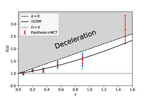
Figure 1: The Pantheon+MCT SNe Ia measurements on $E(z)$ with $1\sigma$, $2\sigma$ and $3\sigma$ errors. The dashed line corresponds to the $Rh=ct$ model with $q(z)=0$, the dotted line denotes $E(z)=1$ which represents the model with $\dot{H}=0$ in a spatially flat universe, and the solid line shows the best fit $\Lambda$CDM model.

Then we compare the CCH measurements on the Hubble parameter $H(z)$ with the null hypothesis (2.3) and (2.5) and the result is shown in figure 2. Since the Hubble constant $H_{0}$ appears in equations (2.3) and (2.5), and the latest result $H_{0}=67.27\pm 0.60$ km/s/Mpc from Planck 2018 [21] is in tension with the local measurement $H_{0}=74.03\pm 1.42$ km/s/Mpc from HST [22] at $4.4\sigma$ level, so the direct evidence of cosmic acceleration from CCH data is affected by the uncertainty in $H_{0}$ and this method depends on the cosmological model as the way the Hubble constant depends on. In figure 2, we take both the values $H_{0}=67.27\pm 0.60$ km/s/Mpc and $H_{0}=74.03\pm 1.42$ km/s/Mpc. For $H_{0}=74.03$ km/s/Mpc, some of the low redshift $(z<1)$ CCH data violate the lower bound of the null hypothesis (2.5), and the three points at $z=0.68$, $z=0.781$ and $z=1.53$ violate the lower bound even at $2\sigma$ confidence level. So we expect that the Universe once experienced accelerated expansion, but this does not mean that the accelerated expansion happened up to $z=1.53$. For $H_{0}=67.27$ km/s/Mpc, the data points that violate the lower bound (2.5) become less and only two points at $z=0.68$ and $z=1.53$ violate the lower bound at $2\sigma$ confidence level. Therefore, the evidence strongly depends on the value of $H_{0}$. For both choices of $H_{0}$, we see $2\sigma$ evidence of cosmic acceleration and no strong evidence of super-accelerated expansion, note that this result applies to any value of $\Omega_{k}$. Comparing with the evidence from $E(z)$ data, this evidence is much weaker and it depends on the value of $H_{0}$ as discussed above. On the other hand, we may argue that those points which violate the lower bound are outliers, so we fit the $Rh=ct$ model to the CCH data and we get the best fit $H_{0}=62.34\pm 1.43$ km/s/Mpc and $\chi^{2}=16.62$. For the $\Lambda$CDM model, the best fit is $\Omega_{m0}=0.32\pm 0.06$, $H_{0}=68.11\pm 3.09$ km/s/Mpc and $\chi^{2}=14.50$. In terms of $\chi^{2}$ statistics, it seems that both $Rh=ct$ and $\Lambda$CDM model fit CCH data well. To avoid the possible outlier problem, in the next section we reconstruct the data using the GP method.

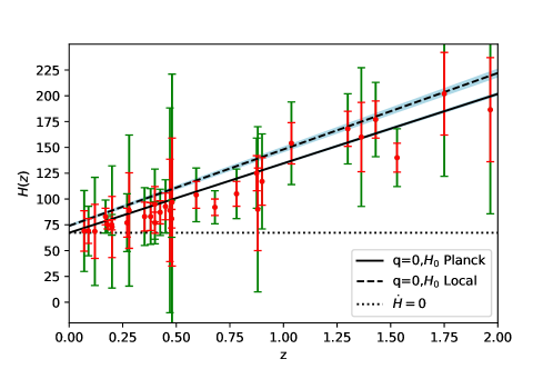
Figure 2: The CCH data with $1\sigma$ and 2$\sigma$ uncertainties. The solid lines corresponds to $q(z)=0$ with $H_{0}=67.27$ km/s/Mpc and the blue shaded area corresponds to $H_{0}=67.27\pm 0.60$ km/s/Mpc. The dotted line denotes $H(z)=H_{0}=67.27$ km/s/Mpc. The dashed line corresponds to $q(z)=0$ with $H_{0}=74.03$ km/s/Mpc and the blue shaded area corresponds to $H_{0}=74.03\pm 1.42$ km/s/Mpc.

3 Reconstruction of observational data with Gaussian process

Although we conclude that the Universe once experienced accelerated expansion just by comparing $E(z)$ data with the bound $1+z$, we have no idea on the property of cosmic acceleration like when the cosmic acceleration began. In this section, we use the GP method to reconstruct $E(z)$ and $q(z)$. The detailed discussion of GP method is presented in appendix B. Since there are only six $E(z)$ data, so we reconstruct $E(z)$ by combining the CCH data on the Hubble parameter and the Pantheon+MCT data on $E(z)$ to show direct evidence of cosmic acceleration. As seen from equation (2.5), to derive $E(z)=H(z)/H_{0}$ from $H(z)$, we need to determine the Hubble constant $H_{0}$ from the reconstructed $H(z)$ function at $z=0$ by using the 31 CCH data. We use the inferred value of $H_{0}=67.46\pm 4.75$ km/s/Mpc from the GP reconstruction of the CCH data and divide the CCH data by this $H_{0}$ to obtain $E(z)$ from the CCH data, then we add these $E(z)$ data to the Pantheon+MCT data to reconstruct $E(z)$ function. The result is shown in figure 3. The reconstructed value $H_{0}=67.46\pm 4.75$ km/s/Mpc is consistent with the result $H_{0}\sim 67\pm 4$ km/s/Mpc obtained from the 31 CCH data and 5 BAO data with the GP method in [25]. It is also consistent with reconstructed result $H_{0}=67.06\pm 1.68$ km/s/Mpc obtained from the combination of CCH and SNe Ia data in [28]. Because the reconstruction starts from $z=0$ and $E(z=0)=1$ by definition, we expect the convergence at $E(z=0)=1$ due to the Hubble law $H(z)\approx H_{0}$ at low redshift which is independent of cosmological models to the lowest order. However, the large uncertainties in $H(z)$ decrease the constraint ability of this method near $z=0$. From figure 3, we see $3\sigma$ evidence of accelerated expansion in the redshift ranges $0.1\lesssim z\lesssim 1$, but no significant evidence for decelerated expansion. Again the results don’t mean that in the redshift ranges $0.1\lesssim z\lesssim 1$ the universe always experienced accelerated expansion.

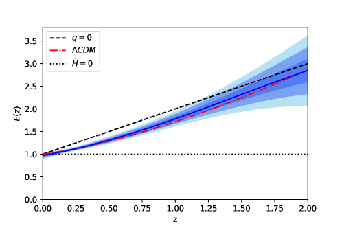
Figure 3: GP reconstruction of $E(Z)$ from CCH+Patheon+MCT data. The blue solid line is the mean of the reconstruction and the shaded areas are $1\sigma$, $2\sigma$ and $3\sigma$ errors. The dashed line corresponds to $q(z)=0$ ($E(z)=1+z$) and the dotted line corresponds to $E(z)=1$.

In order to get detailed information about the acceleration and the transition redshift, we reconstruct the deceleration parameter $q(z)$ from the reconstructed $E(z)$ and $E^{\prime}(z)$ by using the relation $q(z)=E^{\prime}(z)(1+z)/E(z)-1$, and the result is shown in figure 4. We see that accelerated expansion happened until $z\lesssim 0.3$ at the $2\sigma$ level. The mean of reconstruction suggests that the transition from deceleration to acceleration happened at $z_{t}=0.60_{-0.12}^{+0.21}$. It is consistent with the result $0.33<z_{t}<1.0$ obtained in [25] and our constraint is more stringent due to the addition of SNe Ia data.

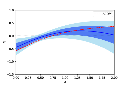
Figure 4: GP reconstruction of the deceleration parameter $q(z)$ from CCH+Pantheon+MCT. The blue solid line is the mean of the reconstruction and the shaded areas are $1\sigma$ and $2\sigma$ errors. The dashed line corresponds to $\Lambda CDM$ model and the dotted line corresponds to $q(z)=0$.

4 Observational constraints on acceleration and dark energy

To better understand the properties of acceleration and dark energy and to measure cosmological parameters, we use two particular parameterizations to fit the combination of SNe Ia, $H(z)$ and BAO data in this section. We first consider a simple parametrization of the deceleration parameter $q(z)$ [81]

$$q(z)=\frac{1}{2}+\frac{q_{1}z+q_{2}}{(1+z)^{2}}.$$ (4.1)

In this model, $q_{0}=1/2+q_{2}$. Substituting equation (4.1) into equation (2.4), we get

$$H(z)=H_{0}(1+z)^{\frac{3}{2}}\exp\left[\frac{q_{2}}{2}+\frac{q_{1}z^{2}-q_{2}}{2(1+z)^{2}}\right].$$ (4.2)

To fit the model to CCH data, we calculate

$$\chi_{H}^{2}=\sum_{i}\frac{[H_{obs}(z_{i})-H_{th}(z_{i})]^{2}}{\sigma_{i}^{2}}.$$ (4.3)

For the SNe Ia data, we consider the distance modulus measurements from Pantheon compilation and the expansion rate measurements from Pantheon+MCT separately. For the Pantheon+MCT data, we calculate

$$\chi_{SN}^{2}=\sum_{ij}[E_{obs}(z_{i})-E_{th}(z_{i})]C_{E}^{-1}(z_{i},z_{j})[E_{obs}(z_{j})-E_{th}(z_{j})],$$ (4.4)

For the distance modulus data, we combine equations (4.2) and (A.6) to get the distance modulus $\mu_{th}=5\log_{10}[d_{L}(z)/\text{Mpc}]+25$, then we calculate

$$\chi_{SN}^{2}=\Delta\mu^{T}\cdot\Sigma_{\mu}^{-1}\cdot\Delta\mu,$$ (4.5)

where $\Delta\mu=\mu_{obs}-\mu_{th}$ and $\Sigma_{\mu}$ is the total covariance matrix. Finally, the total chi-square is given by

$$\chi^{2}=\chi_{H}^{2}+\chi_{SN}^{2}$$ (4.6)

Unlike the parametrization of the equation of state, the parameters $\Omega_{m0}$ and $\Omega_{b}$ are absent in equation (4.2) and they are not model parameters, but we need them to calculate the sound horizon at the drag redshift for the BAO parameters, so we don’t use the BAO data for this model.

Fitting the model to CCH+Pantheon and CCH+Pantheon+MCT, we obtain the constraints on the model parameters $q_{1}$ and $q_{2}$ along with the Hubble constant and the results are shown in figure 5. The $1\sigma$ constraints on the model parameters are shown in table 1. From table 1 and figure 5, we see that the constraints on the model parameters $H_{0}$, $q_{1}$ and $q_{2}$ are very similar with either CCH+Pantheon or CCH+Pantheon+MCT data and the results are consistent, so we can replace the full distance modulus data by the compressed expansion rate data. The Hubble constant is consistent with the Planck 2018 result.

For comparison, we also fit the curved $\Lambda$CDM model and $Rh=ct$ model to the CCH+Pantheon data. Because the Patheon+MCT data assume a spatially flat universe, so we don’t fit the curved $\Lambda$CDM model and $Rh=ct$ model to this data. For the curved $\Lambda$CDM model, we get $H_{0}=69.4\pm 2.0$ km/s/Mpc, $\Omega_{m0}=0.33\pm 0.06$, $\Omega_{k0}=-0.08\pm 0.16$ and $\chi^{2}=1050.37$, this result is also shown in table 2. For the $Rh=ct$ model, we get $H_{0}=62.34\pm 1.43$ km/s/Mpc and $\chi^{2}=1140.65$. Both the simple $q(z)$ and the curved $\Lambda$CDM models fit the data well and the Hubble constant is consistent with Planck 2018 result. In terms of Akaike Information Criterion (AIC) which is defined as $\chi^{2}+2n$, where $n$ is the number of parameters in the model, we get AIC=1056.37 for the curved $\Lambda$CDM model and AIC=1142.65 for the $Rh=ct$ model. So comparing with the simple $q(z)$ model and the curved $\Lambda$CDM model, the $Rh=ct$ model is strongly disfavored by the CCH+Pantheon data.

Table 1: The $1\sigma$ constraints on the model parameters for the simple $q(z)$ model. QDa denotes the data sets CCH+Pantheon and QDb denotes the data sets CCH+Pantheon+MCT.

Data sets	$H_{0}$ (km/s/Mpc)	$q_{1}$	$q_{2}$	$\chi^{2}$	AIC
QDa	$69.14\pm 1.86$	$-0.19\pm 0.43$	$-1.18\pm 0.10$	1050.77	1056.77
QDb	$69.38\pm 1.87$	$-0.21\pm 0.44$	$-1.18\pm 0.11$	20.86	26.86

Table 2: The $1\sigma$ constraints on the model parameters for the $\Lambda$CDM model. QDa denotes the data sets CCH+Pantheon and SDa denotes the data sets CCH+BAO+Pantheon.

Data sets	$H_{0}$ (km/s/Mpc)	$\Omega_{m0}$	$\Omega_{k0}$	$\chi^{2}$	AIC
QDa	$69.4\pm 2.0$	$0.33\pm 0.06$	$-0.08\pm 0.16$	1050.37	1056.67
SDa	$68.9\pm 1.8$	$0.325\pm 0.014$	$-0.09\pm 0.05$	1065.63	1071.63

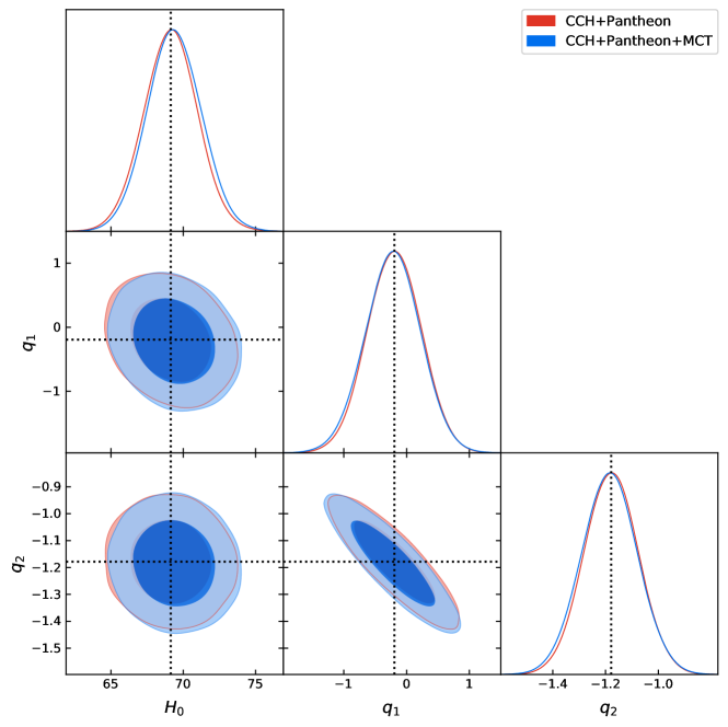
Figure 5: The $1\sigma$ and $2\sigma$ contour plots for the simple $q(z)$ model.

By using the observational constraints, we reconstruct $q(z)$ and the result is shown in figure 6. Figure 6 shows $3\sigma$ evidence for cosmic acceleration in the redshift ranages $0\leq z\leq 0.25$ and $2\sigma$ evidence for cosmic deceleration in the past with $z\gtrsim 1$. The transition redshift when the Universe underwent the transition from deceleration to acceleration is $z_{t}=0.61_{-0.16}^{+0.24}$ at the $1\sigma$ confidence level. This result is consistent with that in the last section obtained from GP reconstruction and $\Lambda$CDM model.

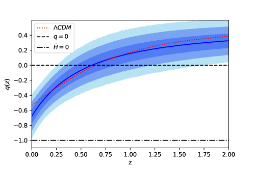
Figure 6: The reconstruction of the deceleration parameter by using the constraints from CCH+Pantheon data for the simple $q(z)$ model. The solid line is drawn by using the best fit parameters. The shaded areas are the $1\sigma$, $2\sigma$ and $3\sigma$ uncertainties. The red dotted line denotes the best fit $\Lambda$CDM model.

To use the BAO data and measure the cosmological parameters, now we consider the SSLCPL model [83, 84]. This model approximates the dynamics of general thawing scalar fields over a large redshift range and it has only one parameter for $w(z)$. It has the same form as the commonly used Chevallier-Polarski-Linder (CPL) model which parameterizes the equation of state parameter as [85, 86]

$$w(z)=w_{0}+w_{a}\frac{z}{1+z}.$$ (4.7)

For the SSLCPL model, the parameter $w_{a}$ is not an independent parameter, i.e.,

$$w_{a}=6(1+w_{0})\frac{(\Omega_{\phi 0}^{-1}-1)[\sqrt{\Omega_{\phi 0}}-\tanh^{-1}(\sqrt{\Omega_{\phi 0}})]}{\Omega_{\phi 0}^{-1/2}-(\Omega_{\phi 0}^{-1}-1)\tanh^{-1}(\sqrt{\Omega_{\phi 0}})},$$ (4.8)

where $\Omega_{\phi 0}$ is the dark energy density normalized by the current critical energy density. The SSLCPL model has only one free parameter $w_{0}$ and it reduces to the $\Lambda$CDM model when the parameter $w_{0}=-1$. With this explicit degeneracy relation between $w_{0}$ and $w_{a}$, we expect to get tighter constraints on $\Omega_{\phi 0}$ and $w_{0}$ for the SSLCPL model than the CPL model does. For a spatially flat universe, the Friedmann equation for the CPL parametrization becomes

$$\begin{split}\frac{H^{2}}{H_{0}^{2}}=&\Omega_{r0}(1+z)^{4}+\Omega_{m0}(1+z)^{3}+\\ &(1-\Omega_{r0}-\Omega_{m0})(1+z)^{3(1+w_{0}+w_{a})}\exp(\frac{-3w_{a}z}{1+z}),\end{split}$$ (4.9)

where $\Omega_{r0}$ is radiation density parameter, $\Omega_{m0}$ is matter density parameter and $1-\Omega_{r0}-\Omega_{m0}=\Omega_{\phi 0}$ is the dark energy density parameter. To fit the flat SSLCPL model to the observational data and obtain the best fit parameters, we minimize

$$\chi^{2}=\chi_{H}^{2}+\chi_{SN}^{2}+\chi_{BAO}^{2}.$$ (4.10)

The results for fitting both the CCH+BAO+Pantheon data (we label this data sets as SDa) and CCH+BAO+Pantheon+MCT data (we label this data sets as SDb) are shown in figure 7 and table 3. From figure 7 and table 3, we see that the constraints on the model parameters from both SDa and SDb data are very similar and they are consistent, and both results are consistent with flat $\Lambda$CDM model. As shown in tables 2 and 3, both flat SSLCPL and curved $\Lambda$CDM model fit the observational data well.

Table 3: The $1\sigma$ constraints on the model parameters for the SSLCPL model. SDa denotes the data sets CCH+BAO+Pantheon and SDb denotes the data sets CCH+BAO+Pantheon+MCT.

Data sets	$H_{0}$ (km/s/Mpc)	$\Omega_{\phi 0}$	$w_{0}$	$\chi^{2}$	AIC
SDa	$66.79\pm 1.40$	$0.687\pm 0.013$	$-1.03\pm 0.07$	1068.48	1074.48
SDb	$66.90\pm 1.39$	$0.688\pm 0.013$	$-1.04\pm 0.07$	38.85	44.85

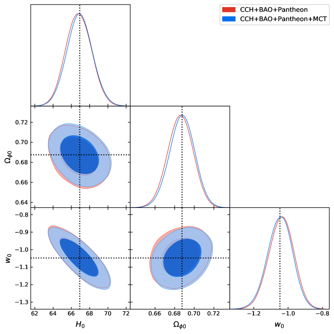
Figure 7: The $1\sigma$ and $2\sigma$ contour plots for the SSLCPL model.

5 Discussion

The null hypothesis that cosmic acceleration never happened gives the kinematic bound $E(z)\geq 1+z$. In standard cosmology, the null hypothesis $q(z)\geq 0$ is equivalent to the strong energy condition $\rho+3p\geq 0$. The six $E(z)$ data from Patheon+MCT can be compared directly with the lower bound to give direct evidence of cosmic acceleration. The five low redshfit data points with $z<1$ lie outside the lower bound at the $3\sigma$ confidence level, and the only one high redshift data crosses the bound at the $1\sigma$ level. Therefore, we have $3\sigma$ direct evidence of cosmic acceleration. This direct evidence does not assume any gravitational theory or cosmological model. The only caveat from this direct evidence is that the $E(z)$ assumes a spatially flat universe. Although there is no strong evidence for decelerated expansion, it does not mean the cosmic acceleration started at least from $z\sim 0.9$ or there is no decelerated expansion in the redshift ranges $0<z<0.9$ because of the integration effect of the deceleration parameter. Due to the integration effect, even if the transition from cosmic acceleration to deceleration happened at the redshift $z\sim 0.6$, the expansion rate remains outside the bound until $z\gtrsim 2$. The direct evidence does exclude the $Rh=ct$ at the $3\sigma$ confidence level. Comparing the $Rh=ct$ model with $\Lambda$CDM model by the $\chi^{2}$ statistics, the $Rh=ct$ model is also strongly disfavoured by the $E(z)$ data. We also use the CCH data to give direct evidence of cosmic acceleration. Due to large error bars in the data and the uncertainties in the value of the Hubble constant, only several data points lie outside the lower bound. Those data points may be outliers, so the evidence from CCH data is not convincing.

The GP method was used to reconstruct the $E(z)$ and $q(z)$ functions from the CCH and Pantheon+MCT data. The Hubble constant $H_{0}=67.46\pm 4.75$ km/s/Mpc inferred from the reconstructed $H(z)$ by CCH data is consistent with the Planck 2018 result, but it has a little tension with the local measurement even though the error bar is big. The reconstructed $E(z)$ shows more than $3\sigma$ direct evidence for cosmic acceleration up to the redshift $z\sim 1$, and the reconstructed $q(z)$ function gives the transition redshift $z_{t}=0.60_{-0.12}^{+0.21}$ at which the expansion of the Universe underwent the transition from acceleration to deceleration.

Fitting the simple two-parameter parametrization $q(z)=1/2+(q_{1}z+q_{2})/(1+z)^{2}$ to CCH+Patheon and CCH+Patheon+MCT data we get consistent constraints on the model parameters. The best fit Hubble constant is $H_{0}=69.14\pm 1.86$ km/s/Mpc. This value is consistent with the Planck 2018 result and has a little tension with the local measurement. By using the fitted parameters from CCH+Patheon, we reconstruct $q(z)$ and get the transition redshift $z_{t}=0.61^{+0.24}_{-0.16}$ which is consistent with that from GP method. We also fit the SSLCPL model to the combination of CCH, BAO and SNe Ia data, and we get consistent results with either Pantheon or Patheon+MCT data. The Hubble constant $H_{0}=66.79\pm 1.4$ km/s/Mpc from fitting the SSLCPL model to the CCH+BAO+Pantheon data is consistent with the Planck 2018 result and is in tension with the local measurement at $3.6\sigma$ confidence level. The addition of the type Ia SNe data helps the CCH and BAO data to tighten the error bar on the Hubble constant, but it does not affect the value of the Hubble constant because of the arbitrary normalization of the luminosity distance.

In conclusion, the expansion rate measured from Pantheon+MCT gives more than $3\sigma$ direct evidence for cosmic acceleration. In fitting cosmological models, we can use the six compressed data points on the expansion rate instead of the full Pantheon compilation. The CCH and BAO data prefers lower value of the Hubble constant which is consistent with Planck 2018 result.

Appendix A Observational data

The Hubble parameter directly probes the expansion history of the Universe by its definition $H=\dot{a}/a$, where $a$ denotes the cosmic scale factor and $\dot{a}$ is its rate of change with respect to the cosmic time $t$. Since the Hubble parameter is related with the differential redshift time as

$$H(z)=-\frac{1}{(1+z)}\frac{dz}{dt}\approx-\frac{1}{(1+z)}\frac{\Delta z}{\Delta t},$$ (A.1)

and $dz$ is obtained from spectroscopic surveys, so a measurement of $dt$ gives the Hubble parameter which is independent of the cosmological model. Based on the spectroscopic differential evolution of passively evolving galaxies, CCH method obtains the expansion rate $dz/dt$ by taking a pair of massive and passively evolving galaxies at two different redshifts [87]. We show the 31 CCH data points of $H(z)$ compiled by [88, 25, 38, 29, 28, 89] in table 4. These data cover a redshift range up to $z\sim 2$ and are obtained without assuming any particular cosmological model. There exit systematic uncertainties associated with the stellar population synthesis models like BC03 [90] and MaStro [91], and a possible contamination due to young underlying stellar components in quiescent galaxies [89], so the data is model dependent in this sense. Here we use the measurements on $H(z)$ with the BC03 model. To keep the data to be model independent as minimum as possible, we don’t use the $H(z)$ data determined by BAO measurements in this paper.

Table 4: The 31 CCH data with the BC03 model. The unit for $H(z)$ is km/s/Mpc.

$z$	$H(z)$	$\sigma_{H(z)}$	Ref.		$z$	$H(z)$	$\sigma_{H(z)}$	Ref.
0.07	69.0	19.6	[92]		0.4783	80.9	9.0	[93]
0.09	69.0	12.0	[94]		0.48	97.0	62.0	[95]
0.12	68.6	26.2	[92]		0.593	104.0	13.0	[96]
0.17	83.0	8.0	[94]		0.68	92.0	8.0	[96]
0.179	75.0	4.0	[96]		0.781	105.0	12.0	[96]
0.199	75.0	5.0	[96]		0.875	125.0	17.0	[96]
0.2	72.9	29.6	[92]		0.88	90.0	40.0	[95]
0.27	77.0	14.0	[94]		0.9	117.0	23.0	[94]
0.28	88.8	36.6	[92]		1.037	154.0	20.0	[96]
0.352	83.0	14.0	[96]		1.3	168.0	17.0	[94]
0.3802	83.0	13.5	[93]		1.363	160.0	33.6	[97]
0.4	95.0	17.0	[94]		1.43	177.0	18.0	[94]
0.4004	77.0	10.2	[93]		1.53	140.0	14.0	[94]
0.4247	87.1	11.2	[93]		1.75	202.0	40.0	[94]
0.4497	92.8	12.9	[93]		1.965	186.5	50.4	[97]
0.47	89.0	49.6	[98]

The Pantheon sample [26] is the largest SNe Ia sample which includes 1048 spectroscopically confirmed SNe Ia and the furthest SN reaches approximately redshift $z\sim 2.3$. It consists of 279 spectroscopically confirmed SNe Ia with redshift $0.03<z<0.68$ discovered by the Pan-STARRS1 Medium Deep Survey [99], samples of SNe Ia from the Harvard Smithsonian Center for Astrophysics SN surveys [100], the Carnegie SN Project [101], the Sloan digital sky survey [102] and the SN legacy survey [103], and high-z data with the redshift $z>1.0$ from the Hubble space telescope cluster SN survey [104], GOODS [105] and CANDELS/CLASH survey [106, 107]. The calibration systematics is reduced substantially by cross-calibrating all of the SN samples. The distance modulus $\mu$ of SNe Ia was derived from the observation of light curves through the SALT2 light-curve fitter

$$\mu_{obs}=m_{B}-M_{B}+\alpha\cdot X_{1}-\beta\cdot C+\Delta_{M}+\Delta_{B},$$ (A.2)

where $m_{B}$ corresponds to the observed peak magnitude in rest-frame $B$ band, $X_{1}$ is the time stretching of the light curve, $C$ describes the supernova color at maximum brightness, $M_{B}$ is the absolute $B$-band magnitude of a fiducial SN Ia with $X_{1}=0$ and $C=0$, $\Delta_{M}$ is a distance correction based on the host-galaxy mass of the SN and $\Delta_{B}$ is a distance correction based on predicted biases from simulations. The parameters $\alpha$ and $\beta$ characterize luminosity-stretch, and luminosity-color relations. Since the absolute magnitude of a SN Ia is degenerated with the Hubble constant, the corrected magnitudes $\mu+M_{B}$ are given for cosmological model fitting [26]. The nuisance parameters $\alpha$, $\beta$ and $H_{0}$ should be marginalized. The statistical uncertainty and systematic uncertainty are also given in ref. [26]. The total uncertainty matrix of the distance modulus is given by

$$\Sigma_{\mu}=D_{stat}+C_{sys},$$ (A.3)

where the statistical matrix $D_{stat}$ has only a diagonal component and $C_{sys}$ is the systematic covariance. We take into account all the statistical uncertainties as described by their full covariance matrix.

Recently, Riess et al. combine the Pantheon sample with 15 SNe Ia at redshift $z>1$ discovered in the CANDELS and CLASH Multi-Cycle Treasury (MCT) programs using WFC3 on the Hubble Space Telescope and compress the raw distance measurements to expansion rate $E(z)$ at six redshifts in the range $0.07<z<1.5$ by assuming a flat universe with $\Omega_{k}=0$ [27], the results and the correlation matrix of $E(z)$ are shown in table 5. Because of the assumption of a flat universe, the results of $E(z)$ are cosmological model dependent in this sense. The last point $E(z=1.5)$ is not Gaussian, the symmetrization of the upper and lower bounds gives $E(1.5)=2.924\pm 0.675$ [29], or $E(1.5)=2.67\pm 0.675$ [60], and the Gaussian approximation is $E(1.5)=2.78\pm 0.59$ [89].

Table 5: Pantheon+MCT SN Ia measurements of $E(z)$ [27].

$z$	$E(z)$	Correlation Matrix
0.07	$0.994\pm 0.023$	1.00
0.2	$1.113\pm 0.020$	0.40	1.00
0.35	$1.122\pm 0.037$	0.52	-0.13	1.00
0.55	$1.369\pm 0.063$	0.35	0.35	-0.18	1.00
0.9	$1.54\pm 0.12$	0.02	-0.08	0.19	-0.41	1.00
1.5	$2.69^{+0.86}_{-0.52}$	0.00	-0.06	-0.05	0.16	-0.21	1.00

BAO is a powerful standard ruler to probe the angular diameter distance and the Hubble parameter evolution. The isotropic and anisotropic BAO measurements are summarized in tables 6 and 7, respectively [108]. The covariance matrix associated with the data in table 7 is

$$\bm{C}=\begin{pmatrix}0.0150&-0.0357&0.0071&-0.0100&0.0032&-0.0036&0&0\\ -0.0357&0.5304&-0.0160&0.1766&-0.0083&0.0616&0&0\\ 0.0071&-0.0160&0.0182&-0.0323&0.0097&-0.0131&0&0\\ -0.0100&0.1766&-0.0323&0.3267&-0.0167&0.1450&0&0\\ 0.0032&-0.0083&0.0097&-0.0167&0.0243&-0.0352&0&0\\ -0.0036&0.0616&-0.0131&0.1450&-0.0352&0.2684&0&0\\ 0&0&0&0&0&0&0.1358&-0.0296\\ 0&0&0&0&0&0&-0.0296&0.0492\\ \end{pmatrix}.$$

Table 6: Isotropic BAO data.

Data set	Redshift	$D_{V}(z)/r_{d}$	Ref.
6dF	z=0.106	$2.98\pm 0.13$	[109]
MGS	z=0.15	$4.47\pm 0.17$	[110]
eBOSS quasars	z=1.52	$26.1\pm 1.1$	[111]

Table 7: Anisotropic BAO data. In the third column, $A$ means $D_{A}(z)/r_{d}$ and $H$ means $D_{H}(z)/r_{d}$.

Data set	Redshift	$D_{A/H}(z)/r_{d}$	Ref.
BOSS DR12	z=0.38	$7.42(A)$	[112]
BOSS DR12	z=0.38	$24.97(H)$	[112]
BOSS DR12	z=0.51	$8.85(A)$	[112]
BOSS DR12	z=0.51	$22.31(H)$	[112]
BOSS DR12	z=0.61	$9.69(A)$	[112]
BOSS DR12	z=0.61	$20.49(H)$	[112]
BOSS DR12	z=2.4	$10.76(A)$	[113]
BOSS DR12	z=2.4	$8.94(H)$	[113]

In a spatially flat universe, the Hubble distance is

$$D_{H}(z)=\frac{c}{H(z)},$$ (A.4)

the angular diameter distance is

$$D_{A}(z)=\frac{c}{1+z}\int_{0}^{z}\frac{dx}{H(x)},$$ (A.5)

the luminosity distance is

$$d_{L}(z)=c(1+z)\int_{0}^{z}\frac{dx}{H(x)},$$ (A.6)

and the effective distance $D_{V}(z)$ is [114]

$$D_{V}(z)=\left[\frac{d_{L}^{2}(z)}{(1+z)^{2}}\frac{cz}{H(z)}\right]^{1/3}.$$ (A.7)

The sound horizon at the drag redshift $z_{d}$ is

$$r_{d}=\frac{c}{\sqrt{3}}\int_{z_{d}}^{\infty}\frac{dz}{\sqrt{1+(3\Omega_{b}/4\Omega_{\gamma})/(1+z)}H(z)},$$ (A.8)

and the drag redshift $z_{d}$ is fitted as [115]

$$z_{d}=\frac{1291(\Omega_{m}h^{2})^{0.251}}{1+0.659(\Omega_{m}h^{2})^{0.828}}[1+b_{1}(\Omega_{b}h^{2})^{b_{2}}],$$ (A.9)

where

$$b_{1}=0.313(\Omega_{b}h^{2})^{-0.419}[1+0.607(\Omega_{m}h^{2})^{0.674}],$$ (A.10)

and

$$b_{2}=0.238(\Omega_{m}h^{2})^{0.223}.$$ (A.11)

In this work we take $\Omega_{b}h^{2}=0.02236$ and $\Omega_{\gamma}h^{2}=2.469\times 10^{-5}$ [21], where the dimensionless parameter $h=H_{0}/(100$ km/s/Mpc). To use the data, we calculate

$$\chi_{BAO}^{2}=\chi_{iso}^{2}+\chi_{aniso}^{2},$$ (A.12)

$$\chi_{iso}^{2}=\sum_{i}(\frac{v_{i}-d_{i}^{iso}}{\sigma_{i}})^{2},$$ (A.13)

$$\chi_{aniso}^{2}=(\bm{w}-\bm{d}^{aniso})^{T}\bm{C}^{-1}(\bm{w}-\bm{d}^{aniso}),$$ (A.14)

where the vectors $\bm{d}^{iso}$ and $\bm{d}^{aniso}$ are the isotropic and anisotropic data from tables 6 and 7, respectively, and $\bm{v}$ and $\bm{w}$ are the predictions for these vectors in a given cosmological model.

Appendix B Gaussian process method

Because of insufficient and low quality of observational data, we use the GP method to find a smooth function $f(x)$ that best represents a set of observational data points $f(x_{i})\pm\sigma_{i}$. The GP method assume that the value of the function $f(x)$ at any point $x$ follows a Gaussian distribution. At each $z_{i}$, the value of $f(z_{i})$ is drawn from a Gaussian distribution with mean $u(z_{i})$ and variance $k(z_{i},z_{i})$. Besides, $f(z_{i})$ and $f(z_{j})$ are correlated by the covariance function (or kernel function) $k(z_{i},z_{j})$.

A GP is written as

$$f(x)\sim\text{GP}(\mu(x),k(x,x^{\prime})),$$ (B.1)

so the kernel function plays a crucial role in the GP method and must be selected beforehand. In this sense, GP is model dependent although it is independent of cosmological models. There are three widely used kernel functions with two degrees of freedom. The Gaussian/squared-exponential kernel

$$k(x_{i},x_{j})=\sigma_{f}^{2}\,\exp\left(-\frac{(x_{i}-x_{j})^{2}}{2l_{f}^{2}}\right),$$ (B.2)

where $\sigma_{f}$ and $l_{f}$ are hyperparameters. The Cauchy kernel

$$k(x_{i},x_{j})=\frac{\sigma_{f}^{2}l_{f}}{(x_{i}-x_{j})^{2}+l_{f}^{2}}.$$ (B.3)

The Matérn kernel

$$k(x_{i},x_{j})=\sigma_{f}^{2}\frac{2^{1-\nu}}{\Gamma(\nu)}\left(\frac{\sqrt{2\nu(x_{i}-x_{j})^{2}}}{l_{f}}\right)^{\nu}\,K_{\nu}\left(\frac{\sqrt{2\nu(x_{i}-x_{j})^{2}}}{l_{f}}\right),$$ (B.4)

where $K_{\nu}$ is the modified Bessel function with $\nu$ being positive. Here we choose the Gaussian kernel. The hyperparameters are determined from the observed data by minimizing the log likelihood function

$$\begin{split}\ln\mathcal{L}=&\ln p(\bm{y}|\bm{X},\sigma_{f},l)\\ =&-\frac{1}{2}(\bm{y}-\bm{\mu})^{T}[K(\bm{X,X})+C]^{-1}(\bm{y}-\bm{\mu})\\ &-\frac{1}{2}\ln|K(\bm{X,X})+C|-\frac{n}{2}\ln(2\pi),\end{split}$$ (B.5)

where $\bm{X}=[x_{1},x_{2},...,x_{n}]^{T}$ are the inputs, $K(\bm{X,X})$ is the covariance matrix with components $k(x_{i},x_{j})$, $\bm{y}$ is the vector of observed data and $C$ is the covariance matrix of the observed data.

To predict the function values $\bm{f_{*}}=[f_{*1},f_{*2},...,f_{*m}]^{T}$ at the test locations $\bm{X_{*}}=[x_{n+1},x_{n+2},...,x_{n+m}]^{T}$, the predictive normal distribution is

$$p(\bm{f_{*}}|\bm{X},\bm{y},\bm{X_{*}})=\mathcal{N}(\hat{\bm{\mu}},\hat{\Sigma}),$$ (B.6)

$$\hat{\bm{\mu}}=K(\bm{X_{*}},\bm{X})^{T}(K(\bm{X},\bm{x}+C)^{-1}(\bm{y}-\bm{\mu(X)})+\bm{\mu}(\bm{X_{*}}),$$ (B.7)

$$\hat{\Sigma}=K(\bm{X_{*},X_{*}})-K(\bm{X_{*}},\bm{X})^{T}(K(\bm{X,X})+C)^{-1}K(\bm{X_{*},X}).$$ (B.8)

The public available python package GaPP [47] is used to do the GP reconstruction in section 3.

References

- [1] Supernova Search Team collaboration, Observational evidence from supernovae for an accelerating universe and a cosmological constant, Astron. J. 116 (1998) 1009 [astro-ph/9805201].
- [2] Supernova Cosmology Project collaboration, Measurements of and from 42 high redshift supernovae, Astrophys. J. 517 (1999) 565 [astro-ph/9812133].
- [3] G. Dvali, G. Gabadadze and M. Porrati, 4-D gravity on a brane in 5-D Minkowski space, Phys. Lett. B. 485 (2000) 208 [hep-th/0005016].
- [4] S. M. Carroll, V. Duvvuri, M. Trodden and M. S. Turner, Is cosmic speed - up due to new gravitational physics?, Phys. Rev. D 70 (2004) 043528 [astro-ph/0306438].
- [5] S. Nojiri and S. D. Odintsov, Modified gravity with negative and positive powers of the curvature: Unification of the inflation and of the cosmic acceleration, Phys. Rev. D68 (2003) 123512 [hep-th/0307288].
- [6] A. A. Starobinsky, Disappearing cosmological constant in f(R) gravity, JETP Lett. 86 (2007) 157 [0706.2041].
- [7] W. Hu and I. Sawicki, Models of f(R) Cosmic Acceleration that Evade Solar-System Tests, Phys. Rev. D 76 (2007) 064004 [0705.1158].
- [8] C. de Rham, G. Gabadadze and A. J. Tolley, Resummation of Massive Gravity, Phys. Rev. Lett. 106 (2011) 231101 [1011.1232].
- [9] Y. Gong, Cosmology in massive gravity, Commun. Theor. Phys. 59 (2013) 319 [1207.2726].
- [10] S. Weinberg, The Cosmological Constant Problem, Rev. Mod. Phys. 61 (1989) 1.
- [11] B. Ratra and P. Peebles, Cosmological Consequences of a Rolling Homogeneous Scalar Field, Phys. Rev. D 37 (1988) 3406.
- [12] C. Wetterich, Cosmology and the Fate of Dilatation Symmetry, Nucl. Phys. B 302 (1988) 668.
- [13] R. Caldwell, R. Dave and P. J. Steinhardt, Cosmological imprint of an energy component with general equation of state, Phys. Rev. Lett. 80 (1998) 1582 [astro-ph/9708069].
- [14] I. Zlatev, L.-M. Wang and P. J. Steinhardt, Quintessence, cosmic coincidence, and the cosmological constant, Phys. Rev. Lett. 82 (1999) 896 [astro-ph/9807002].
- [15] P. J. Steinhardt, L.-M. Wang and I. Zlatev, Cosmological tracking solutions, Phys. Rev. D 59 (1999) 123504 [astro-ph/9812313].
- [16] V. Sahni and A. A. Starobinsky, The Case for a positive cosmological Lambda term, Int. J. Mod. Phys. D 9 (2000) 373 [astro-ph/9904398].
- [17] E. J. Copeland, M. Sami and S. Tsujikawa, Dynamics of dark energy, Int. J. Mod. Phys. D. 15 (2006) 1753 [hep-th/0603057].
- [18] T. Padmanabhan, Dark energy and gravity, Gen. Rel. Grav. 40 (2008) 529 [0705.2533].
- [19] M. Li, X.-D. Li, S. Wang and Y. Wang, Dark Energy, Commun. Theor. Phys. 56 (2011) 525 [1103.5870].
- [20] M. Benetti and S. Capozziello, Connecting early and late epochs by f(z)CDM cosmography, JCAP 1912 (2019) 008 [1910.09975].
- [21] Planck collaboration, Planck 2018 results. VI. Cosmological parameters, 1807.06209.
- [22] A. G. Riess, S. Casertano, W. Yuan, L. M. Macri and D. Scolnic, Large Magellanic Cloud Cepheid Standards Provide a 1% Foundation for the Determination of the Hubble Constant and Stronger Evidence for Physics beyond CDM, Astrophys. J. 876 (2019) 85 [1903.07603].
- [23] B. F. Schutz, Determining the Hubble Constant from Gravitational Wave Observations, Nature 323 (1986) 310.
- [24] LIGO Scientific, Virgo, 1M2H, Dark Energy Camera GW-E, DES, DLT40, Las Cumbres Observatory, VINROUGE, MASTER collaboration, A gravitational-wave standard siren measurement of the Hubble constant, Nature 551 (2017) 85 [1710.05835].
- [25] H. Yu, B. Ratra and F.-Y. Wang, Hubble Parameter and Baryon Acoustic Oscillation Measurement Constraints on the Hubble Constant, the Deviation from the Spatially Flat CDM Model, the Deceleration–Acceleration Transition Redshift, and Spatial Curvature, Astrophys. J. 856 (2018) 3 [1711.03437].
- [26] D. M. Scolnic et al., The Complete Light-curve Sample of Spectroscopically Confirmed SNe Ia from Pan-STARRS1 and Cosmological Constraints from the Combined Pantheon Sample, Astrophys. J. 859 (2018) 101 [1710.00845].
- [27] A. G. Riess et al., Type Ia Supernova Distances at Redshift 1.5 from the Hubble Space Telescope Multi-cycle Treasury Programs: The Early Expansion Rate, Astrophys. J. 853 (2018) 126 [1710.00844].
- [28] A. Gómez-Valent and L. Amendola, from cosmic chronometers and Type Ia supernovae, with Gaussian Processes and the novel Weighted Polynomial Regression method, JCAP 1804 (2018) 051 [1802.01505].
- [29] B. S. Haridasu, V. V. Luković, M. Moresco and N. Vittorio, An improved model-independent assessment of the late-time cosmic expansion, JCAP 1810 (2018) 015 [1805.03595].
- [30] Q. Gao and Y. Gong, The tension on the cosmological parameters from different observational data, Class. Quant. Grav. 31 (2014) 105007 [1308.5627].
- [31] C. Clarkson, B. Bassett and T. H.-C. Lu, A general test of the Copernican Principle, Phys. Rev. Lett. 101 (2008) 011301 [0712.3457].
- [32] V. Sahni, A. Shafieloo and A. A. Starobinsky, Two new diagnostics of dark energy, Phys. Rev. D. 78 (2008) 103502 [0807.3548].
- [33] C. Zunckel and C. Clarkson, Consistency Tests for the Cosmological Constant, Phys. Rev. Lett. 101 (2008) 181301 [0807.4304].
- [34] S. Nesseris and A. Shafieloo, A model independent null test on the cosmological constant, Mon. Not. Roy. Astron. Soc. 408 (2010) 1879 [1004.0960].
- [35] A. Shafieloo, V. Sahni and A. A. Starobinsky, A new null diagnostic customized for reconstructing the properties of dark energy from BAO data, Phys. Rev. D 86 (2012) 103527 [1205.2870].
- [36] S. Yahya, M. Seikel, C. Clarkson, R. Maartens and M. Smith, Null tests of the cosmological constant using supernovae, Phys. Rev. D89 (2014) 023503 [1308.4099].
- [37] S. Nesseris and D. Sapone, Novel null-test for the cold dark matter model with growth-rate data, Int. J. Mod. Phys. D 24 (2015) 1550045 [1409.3697].
- [38] V. Marra and D. Sapone, Null tests of the standard model using the linear model formalism, Phys. Rev. D 97 (2018) 083510 [1712.09676].
- [39] F. O. Franco, C. Bonvin and C. Clarkson, A null test to probe the scale-dependence of the growth of structure as a test of General Relativity, Mon. Not. Roy. Astron. Soc. 492 (2020) L34 [1906.02217].
- [40] V. Sahni, A. Shafieloo and A. A. Starobinsky, Model independent evidence for dark energy evolution from Baryon Acoustic Oscillations, Astrophys. J. 793 (2014) L40 [1406.2209].
- [41] C. Clarkson and C. Zunckel, Direct reconstruction of dark energy, Phys. Rev. Lett. 104 (2010) 211301 [1002.5004].
- [42] A. Shafieloo, A. G. Kim and E. V. Linder, Gaussian Process Cosmography, Phys. Rev. D 85 (2012) 123530 [1204.2272].
- [43] T. Holsclaw, U. Alam, B. Sanso, H. Lee, K. Heitmann, S. Habib et al., Nonparametric Reconstruction of the Dark Energy Equation of State, Phys. Rev. D 82 (2010) 103502 [1009.5443].
- [44] T. Holsclaw, U. Alam, B. Sanso, H. Lee, K. Heitmann, S. Habib et al., Nonparametric Dark Energy Reconstruction from Supernova Data, Phys. Rev. Lett. 105 (2010) 241302 [1011.3079].
- [45] T. Holsclaw, U. Alam, B. Sanso, H. Lee, K. Heitmann, S. Habib et al., Nonparametric Reconstruction of the Dark Energy Equation of State from Diverse Data Sets, Phys. Rev. D 84 (2011) 083501 [1104.2041].
- [46] M. Bilicki and M. Seikel, We do not live in the universe, Mon. Not. Roy. Astron. Soc. 425 (2012) 1664 [1206.5130].
- [47] M. Seikel, C. Clarkson and M. Smith, Reconstruction of dark energy and expansion dynamics using Gaussian processes, JCAP 1206 (2012) 036 [1204.2832].
- [48] M. Seikel, S. Yahya, R. Maartens and C. Clarkson, Using H(z) data as a probe of the concordance model, Phys. Rev. D86 (2012) 083001 [1205.3431].
- [49] M. Seikel and C. Clarkson, Optimising Gaussian processes for reconstructing dark energy dynamics from supernovae, 1311.6678.
- [50] R. Nair, S. Jhingan and D. Jain, Exploring scalar field dynamics with Gaussian processes, JCAP 1401 (2014) 005 [1306.0606].
- [51] V. C. Busti, C. Clarkson and M. Seikel, Evidence for a Lower Value for from Cosmic Chronometers Data?, Mon. Not. Roy. Astron. Soc. 441 (2014) 11 [1402.5429].
- [52] L. Verde, P. Protopapas and R. Jimenez, The expansion rate of the intermediate Universe in light of Planck, Phys. Dark Univ. 5-6 (2014) 307 [1403.2181].
- [53] Z. Li, J. E. Gonzalez, H. Yu, Z.-H. Zhu and J. S. Alcaniz, Constructing a cosmological model-independent Hubble diagram of type Ia supernovae with cosmic chronometers, Phys. Rev. D 93 (2016) 043014 [1504.03269].
- [54] S. D. P. Vitenti and M. Penna-Lima, A general reconstruction of the recent expansion history of the universe, JCAP 1509 (2015) 045 [1505.01883].
- [55] D. Wang and X.-H. Meng, Model-independent determination on H0 using the latest cosmic chronometer data, Sci. China Phys. Mech. Astron. 60 (2017) 110411 [1610.01202].
- [56] M.-J. Zhang and J.-Q. Xia, Test of the cosmic evolution using Gaussian processes, JCAP 1612 (2016) 005 [1606.04398].
- [57] J.-J. Wei and X.-F. Wu, An Improved Method to Measure the Cosmic Curvature, Astrophys. J. 838 (2017) 160 [1611.00904].
- [58] M. K. Yennapureddy and F. Melia, Reconstruction of the HII Galaxy Hubble Diagram using Gaussian Processes, JCAP 1711 (2017) 029 [1711.03454].
- [59] F. Melia and M. K. Yennapureddy, Model Selection Using Cosmic Chronometers with Gaussian Processes, JCAP 1802 (2018) 034 [1802.02255].
- [60] A. M. Pinho, S. Casas and L. Amendola, Model-independent reconstruction of the linear anisotropic stress , JCAP 1811 (2018) 027 [1805.00027].
- [61] J. F. Jesus, R. Valentim, A. A. Escobal and S. H. Pereira, Gaussian Process Estimation of Transition Redshift, 1909.00090.
- [62] C. A. Bengaly, Evidence for cosmic acceleration with next-generation surveys: A model-independent approach, Mon. Not. Roy. Astron. Soc. (2020) in press [1912.05528].
- [63] M. V. John and K. B. Joseph, Generalized Chen-Wu type cosmological model, Phys. Rev. D 61 (2000) 087304 [gr-qc/9912069].
- [64] F. Melia, The Cosmic Horizon, Mon. Not. Roy. Astron. Soc. 382 (2007) 1917 [0711.4181].
- [65] F. Melia and A. Shevchuk, The Universe, Mon. Not. Roy. Astron. Soc. 419 (2012) 2579 [1109.5189].
- [66] M. Lopez-Corredoira, F. Melia, E. Lusso and G. Risaliti, Cosmological test with the QSO Hubble diagram, Int. J. Mod. Phys. D 25 (2016) 1650060 [1602.06743].
- [67] F. Melia, The Linear Growth of Structure in the Universe, Mon. Not. Roy. Astron. Soc. 464 (2017) 1966 [1609.08576].
- [68] F. Melia, A comparison of the Rh = ct and CDM cosmologies using the cosmic distance duality relation, Mon. Not. Roy. Astron. Soc. 481 (2018) 4855 [1804.09906].
- [69] M. V. John, and the eternal coasting cosmological model, Mon. Not. Roy. Astron. Soc. 484 (2019) L35 [1902.05088].
- [70] M. K. Yennapureddy and F. Melia, A comparison of the and CDM cosmologies based on the observed halo mass function, Eur. Phys. J. C 79 (2019) 571 [1907.00897].
- [71] S. Capozziello, Ruchika and A. A. Sen, Model independent constraints on dark energy evolution from low-redshift observations, Mon. Not. Roy. Astron. Soc. 484 (2019) 4484 [1806.03943].
- [72] R. Arjona and S. Nesseris, What can Machine Learning tell us about the background expansion of the Universe?, 1910.01529.
- [73] M. Visser, Energy conditions in the epoch of galaxy formation, Science 276 (1997) 88 [1501.01619].
- [74] M. Visser, General relativistic energy conditions: The Hubble expansion in the epoch of galaxy formation, Phys. Rev. D 56 (1997) 7578 [gr-qc/9705070].
- [75] J. Santos, J. S. Alcaniz and M. J. Reboucas, Energy Conditions and Supernovae Observations, Phys. Rev. D 74 (2006) 067301 [astro-ph/0608031].
- [76] J. Santos, J. S. Alcaniz, N. Pires and M. J. Reboucas, Energy Conditions and Cosmic Acceleration, Phys. Rev. D 75 (2007) 083523 [astro-ph/0702728].
- [77] Y. Gong and A. Wang, Energy conditions and current acceleration of the universe, Phys. Lett. B 652 (2007) 63 [0705.0996].
- [78] Y. Gong, A. Wang, Q. Wu and Y.-Z. Zhang, Direct evidence of acceleration from distance modulus redshift graph, JCAP 0708 (2007) 018 [astro-ph/0703583].
- [79] M. Seikel and D. J. Schwarz, How strong is the evidence for accelerated expansion?, JCAP 0802 (2008) 007 [0711.3180].
- [80] H. Velten, S. Gomes and V. C. Busti, Gauging the cosmic acceleration with recent type Ia supernovae data sets, Phys. Rev. D97 (2018) 083516 [1801.00114].
- [81] Y. Gong and A. Wang, Observational constraints on the acceleration of the universe, Phys. Rev. D 73 (2006) 083506 [astro-ph/0601453].
- [82] Y.-G. Gong and A. Wang, Reconstruction of the deceleration parameter and the equation of state of dark energy, Phys. Rev. D75 (2007) 043520 [astro-ph/0612196].
- [83] Q. Gao and Y. Gong, Constraints on slow-roll thawing models from fundamental constants, Int. J. Mod. Phys. D22 (2013) 1350035 [1212.6815].
- [84] Y. Gong and Q. Gao, On the effect of the degeneracy among dark energy parameters, Eur. Phys. J. C74 (2014) 2729 [1301.1224].
- [85] M. Chevallier and D. Polarski, Accelerating universes with scaling dark matter, Int. J. Mod. Phys. D 10 (2001) 213 [gr-qc/0009008].
- [86] E. V. Linder, Exploring the expansion history of the universe, Phys. Rev. Lett. 90 (2003) 091301 [astro-ph/0208512].
- [87] R. Jimenez and A. Loeb, Constraining cosmological parameters based on relative galaxy ages, Astrophys. J. 573 (2002) 37 [astro-ph/0106145].
- [88] O. Farooq, F. R. Madiyar, S. Crandall and B. Ratra, Hubble Parameter Measurement Constraints on the Redshift of the Deceleration–acceleration Transition, Dynamical Dark Energy, and Space Curvature, Astrophys. J. 835 (2017) 26 [1607.03537].
- [89] A. Gómez-Valent, Quantifying the evidence for the current speed-up of the Universe with low and intermediate-redshift data. A more model-independent approach, JCAP 1905 (2019) 026 [1810.02278].
- [90] G. Bruzual and S. Charlot, Stellar population synthesis at the resolution of 2003, Mon. Not. Roy. Astron. Soc. 344 (2003) 1000 [astro-ph/0309134].
- [91] C. Maraston and G. Stromback, Stellar population models at high spectral resolution, Mon. Not. Roy. Astron. Soc. 418 (2011) 2785 [1109.0543].
- [92] C. Zhang, H. Zhang, S. Yuan, T.-J. Zhang and Y.-C. Sun, Four new observational data from luminous red galaxies in the Sloan Digital Sky Survey data release seven, Res. Astron. Astrophys. 14 (2014) 1221 [1207.4541].
- [93] M. Moresco, L. Pozzetti, A. Cimatti, R. Jimenez, C. Maraston, L. Verde et al., A 6% measurement of the Hubble parameter at : direct evidence of the epoch of cosmic re-acceleration, JCAP 1605 (2016) 014 [1601.01701].
- [94] J. Simon, L. Verde and R. Jimenez, Constraints on the redshift dependence of the dark energy potential, Phys. Rev. D71 (2005) 123001 [astro-ph/0412269].
- [95] D. Stern, R. Jimenez, L. Verde, M. Kamionkowski and S. A. Stanford, Cosmic Chronometers: Constraining the Equation of State of Dark Energy. I: H(z) Measurements, JCAP 1002 (2010) 008 [0907.3149].
- [96] M. Moresco et al., Improved constraints on the expansion rate of the Universe up to z 1.1 from the spectroscopic evolution of cosmic chronometers, JCAP 1208 (2012) 006 [1201.3609].
- [97] M. Moresco, Raising the bar: new constraints on the Hubble parameter with cosmic chronometers at z2, Mon. Not. Roy. Astron. Soc. 450 (2015) L16 [1503.01116].
- [98] A. L. Ratsimbazafy, S. I. Loubser, S. M. Crawford, C. M. Cress, B. A. Bassett, R. C. Nichol et al., Age-dating Luminous Red Galaxies observed with the Southern African Large Telescope, Mon. Not. Roy. Astron. Soc. 467 (2017) 3239 [1702.00418].
- [99] A. Rest et al., Cosmological Constraints from Measurements of Type Ia Supernovae discovered during the first 1.5 yr of the Pan-STARRS1 Survey, Astrophys. J. 795 (2014) 44 [1310.3828].
- [100] M. Hicken, P. Challis, S. Jha, R. P. Kirsher, T. Matheson, M. Modjaz et al., CfA3: 185 Type Ia Supernova Light Curves from the CfA, Astrophys. J. 700 (2009) 331 [0901.4787].
- [101] M. D. Stritzinger et al., The Carnegie Supernova Project: Second Photometry Data Release of Low-Redshift Type Ia Supernovae, Astron. J. 142 (2011) 156 [1108.3108].
- [102] R. Kessler et al., First-year Sloan Digital Sky Survey-II (SDSS-II) Supernova Results: Hubble Diagram and Cosmological Parameters, Astrophys. J. Suppl. 185 (2009) 32 [0908.4274].
- [103] SNLS collaboration, Supernova Constraints and Systematic Uncertainties from the First 3 Years of the Supernova Legacy Survey, Astrophys. J. Suppl. 192 (2011) 1 [1104.1443].
- [104] Supernova Cosmology Project collaboration, The Hubble Space Telescope Cluster Supernova Survey: V. Improving the Dark Energy Constraints Above and Building an Early-Type-Hosted Supernova Sample, Astrophys. J. 746 (2012) 85 [1105.3470].
- [105] A. G. Riess et al., New Hubble Space Telescope Discoveries of Type Ia Supernovae at : Narrowing Constraints on the Early Behavior of Dark Energy, Astrophys. J. 659 (2007) 98 [astro-ph/0611572].
- [106] S. A. Rodney et al., Type Ia Supernova Rate Measurements to Redshift 2.5 from CANDELS : Searching for Prompt Explosions in the Early Universe, Astron. J. 148 (2014) 13 [1401.7978].
- [107] O. Graur et al., Type-Ia Supernova Rates to Redshift 2.4 from CLASH: the Cluster Lensing And Supernova survey with Hubble, Astrophys. J. 783 (2014) 28 [1310.3495].
- [108] J. Evslin, A. A. Sen and Ruchika, Price of shifting the Hubble constant, Phys. Rev. D 97 (2018) 103511 [1711.01051].
- [109] F. Beutler, C. Blake, M. Colless, D. H. Jones, L. Staveley-Smith, L. Campbell et al., The 6dF Galaxy Survey: Baryon Acoustic Oscillations and the Local Hubble Constant, Mon. Not. Roy. Astron. Soc. 416 (2011) 3017 [1106.3366].
- [110] A. J. Ross, L. Samushia, C. Howlett, W. J. Percival, A. Burden and M. Manera, The clustering of the SDSS DR7 main Galaxy sample – I. A 4 per cent distance measure at , Mon. Not. Roy. Astron. Soc. 449 (2015) 835 [1409.3242].
- [111] M. Ata et al., The clustering of the SDSS-IV extended Baryon Oscillation Spectroscopic Survey DR14 quasar sample: first measurement of baryon acoustic oscillations between redshift 0.8 and 2.2, Mon. Not. Roy. Astron. Soc. 473 (2018) 4773 [1705.06373].
- [112] BOSS collaboration, The clustering of galaxies in the completed SDSS-III Baryon Oscillation Spectroscopic Survey: cosmological analysis of the DR12 galaxy sample, Mon. Not. Roy. Astron. Soc. 470 (2017) 2617 [1607.03155].
- [113] H. du Mas des Bourboux et al., Baryon acoustic oscillations from the complete SDSS-III Ly-quasar cross-correlation function at , Astron. Astrophys. 608 (2017) A130 [1708.02225].
- [114] SDSS collaboration, Detection of the Baryon Acoustic Peak in the Large-Scale Correlation Function of SDSS Luminous Red Galaxies, Astrophys. J. 633 (2005) 560 [astro-ph/0501171].
- [115] D. J. Eisenstein and W. Hu, Baryonic features in the matter transfer function, Astrophys. J. 496 (1998) 605 [astro-ph/9709112].