Method of eigenvalue transformation using dispersion oscillating fiber

Abstract

It is known that eigenvalues of Zakharov-Shabat problem can be used to encode a signal in soliton communication lines. We propose to use dispersion oscillation fiber as a new versalite tool to control the eigenvalues. A fiber with sine-wave variation of the core diameter can be used to manage both real and imaginary parts of the eigenvalues. Change of real part of the eigenvalues results in a splitting of an optical breather into two distinct pulses propagating with the different group velocities. Change of imaginary parts of the eigenvalues allows to realize a reverse process of merge of two solitons into high-intensity pulse. The splitting of optical breather and merge of solitons can be obtained even under the strong effect of stimulated Raman scattering. We believe tools and techniques based on use of dispersion oscillating fiber will grant unprecedented control over soliton eigenstates.

1 INTRODUCTION

Optical solitons are formal solutions of nonlinear Schrödinger equation (NLSE) [1, 2, 3]. Using so-called nonlinear Fourier transform [4], a unique set of soliton eigenvalues can be found. Control of soliton eigenvalues has practical application in all-optical routing [1], nonlinear frequency division multiplexing [5, 6, 7], controlled rogue wave generation [8, 9] and in generation of photon entangled pairs [10, 11].

The discrete eigenvalues remain unchanged during interaction of classical Schrödinger solitons. A special type of nonlinearity, dispersion or local perturbation can be used to control soliton eigenstates, soliton amplitudes and velocities [1]. The optical solitons can break up, merge or even annihilate [12, 13, 14, 15]. The role of perturbation can be played by variation of the fiber dispersion or nonlinearity [16, 17], cross-phase modulation in a system of coupled NLS equations [18, 19], and effect of stimulated Raman scattering [20, 21]. Processing of optical pulses via solitons interaction has been analyzed using various nonlinear evolution models [22, 23, 24, 25]. Soliton fusion was observed experimentally [26]. The problem of transforming one optical pulse into another via nonlinear propagation in dispersion varying optical fiber was considered in Ref. 27.

The soliton splitting or soliton fission can be controlled by resonance effects. If the perturbation modulation period is comparable to the oscillation period of a multisoliton pulse, it breaks up into several fundamental solitons [16]. Optical solitons propagating in fibers with a diameter varying along their length satisfy a nonautonomous NLSE with variable dispersion and nonlinearity coefficients [28]. In an NLSE model with a harmonic potential [29], a periodic variation in the potential leads to decay of coupled soliton states. Yan and Dai [30] considered a generalized NLSE with variable coefficients. With different choices of the coefficients, the cubic, periodic, and parabolic solitons can be obtained [31]. Dispersion, nonlinearity and gain coefficients varying in a certain way may lead to the formation of a rogue wave, with a periodic potential as a trigger mechanism [32].

We consider the fission of optical breather and fusion of soliton pair which are initiated by the periodical variation of the fiber dispersion. In our experiments an optical fiber with periodically varying diameter breaks up two-soliton pulse into two fundamental solitons. By changing the modulation of the fiber, one can control the group velocity, centre frequency and peak power of such solitons. Using numerical simulation, we demonstrated that dispersion oscillating fiber can be used for fusion of optical solitons as well. The inelastic soliton interactions driven by variation of the fiber dispersion allow to manage eigenvalues. Our study introduces all-optical tool for processing optical solitons.

2 Nonlinear Schrödinger equation model

To describe the pulse propagation in dispersion oscillating optical fibers with the anomalous dispersion and Kerr-type nonlinearity, one can employ the nonlinear Schrödinger equation model with variable coefficients:

$$\frac{\partial A}{\partial z}+\frac{\alpha}{2}A(z,t)=-\,i\frac{\beta_{2}(z)}{2}\frac{\partial^{2}A}{\partial t^{2}}+\frac{\beta_{3}(z)}{6}\frac{\partial^{3}A}{\partial t^{3}}+i\left({P_{NL}+i\frac{1}{\pi\nu_{0}}\frac{\partial P_{NL}}{\partial t}}\right),$$ (1)

where $A(z,t)$ is the complex pulse envelope, $z$ is the propagation distance; $t$ is the local time in the coordinate system $(z=z,t\to t-z/u)$ [2]; $u$ is the group velocity of the pulse, $\alpha$ is the loss coefficient, and $\nu_{0}$ is the carrier frequency of the pulse. Functions $\beta_{2}(z)$ and $\beta_{3}(z)$ describe dispersion variation which arises due to variation of the fiber diameter. From the measurements of the dispersion of three different fibers drawn from the same preform, but having different diameters, we found following approximations:

$$\beta_{2,3}(z)=\langle\beta_{2,3}\rangle[{1+\beta_{2,3(m)}\;\sin(2\pi\;z/z_{m}+\varphi_{m})}],$$ (2)

where $\langle\beta_{2}\rangle=-12.76\,\mbox{ps}^{2}\mbox{km}^{-1}$, $\langle\beta_{3}\rangle=0.0761\,\mbox{ps}^{3}\mbox{km}^{-1}$, $\beta_{2(m)}=0.02$, $\beta_{3(m)}=0.095$.

Nonlinear media polarization in (1) includes the Kerr effect and delayed Raman scattering $P_{NL}(z,t)=\gamma(z)[(1-f_{R})|A|^{2}A+f_{R}QA(z,t)]$, where $\gamma(z)=\langle\gamma\rangle\left(1+0.028\sin(2\pi z/z_{m})\right),$ $\langle\gamma\rangle=10\,\mbox{W}^{-1}\mbox{km}^{-1}$, $f_{R}=0.18$ [2]. The Raman delayed response $Q(z,t)$ is approximated by damping oscillations associated with a single vibration mode [3]:

$$\frac{\partial^{2}Q}{\partial t^{2}}+\frac{2}{T_{2}}\frac{\partial Q}{\partial t}+\Omega^{2}Q(z,t)=\Omega^{2}|A(z,t)|^{2},$$ (3)

where $T_{2}=32\,\mbox{fs}$, $\Omega=13.1\,\mbox{THz}$.

In our simulations we assume that fiber loss is compensated $(\alpha=0)$ using, for example, Raman gain [33]. For numerical simulations a split-step Fourier method [34] was used. To suppress the waves reflected from the boundaries of the calculation window, we use absorbing boundary conditions.

The eigenvalues of Zakharov-Shabat problem [4] are associated with soliton solutions of classical NLSE [3]. To obtain information about the soliton content of numerical solution of the NLSE with variable coefficients (1) the modified inverse scattering method [35] was used. Using numerical simulations we obtain eigenvalues as functions of their propagation distance: $\lambda_{j}=\lambda_{j}(z)$. The complex envelope of the $j$-th fundamental soliton is defined as follows:

$$A_{j}(z,t)=R_{j}\,{\rm sech}(\kappa_{j}t-t_{j}-v_{j}z)\exp(i\varphi_{j}(z,t)),$$ (4)

where $R_{j}$ is the soliton amplitude; $\kappa_{j}$ is the inverse soliton duration; $t_{j}$ is the coordinate of the pulse peak, $\varphi_{j}(z,t)$ is the field phase; $v_{j}$ determines the change in the group velocity of the soliton: $v_{g}=(1/u+v_{j})^{-1}$. The amplitude, duration and group velocity of the fundamental soliton (4) can be expressed through the spectral parameters $\lambda_{j}$:

$$R_{j} = \tau_{0}^{-1}(|\beta_{2}|/\gamma)^{1/2}(2Im(\lambda_{j})),$$

$$\kappa_{j} = \tau_{0}^{-1}(2Im(\lambda_{j})),$$ (5)

$$v_{j} = \beta_{2}\tau_{0}^{-1}(2Re(\lambda_{j})),$$

where $\tau_{0}=t_{0}(|\beta_{2}|/\gamma)(|\langle\beta_{2}\rangle|/\langle\gamma\rangle)^{-1}$ is the duration of the fundamental soliton in a waveguide with adiabatic $(z_{m}>>1)$ variations in the parameters $\beta_{2}(z)$ and $\gamma(z)$. Change of the soliton group velocity is associated with the shift of the pulse carrier frequency

$$\Delta\Omega=2\tau_{0}^{-1}Re(\lambda_{j}).$$ (6)

3 Splitting of optical breather

The nonlinear Schrödinger equation in absence of perturbations can support bound states formed by multiple solitons localized at same positions. Such states are known as breathers. For the breather the input field can be described by hyperbolic secant pulse

$$A(0,t)=\frac{N}{t_{0}}\sqrt{\frac{|\beta_{2}|}{\gamma}}{\rm sech}\left(\frac{t}{t_{0}}\right),$$ (7)

where $A(0,t)$ is electric field envelope at the input ($z=0$), $N$ is the soliton order, $t_{0}=T_{{}_{\rm FWHM}}/1.76$ is the width of hyperbolic secant pulse, $T_{{}_{\rm FWHM}}$ is the pulse width at the half of the maximum intensity [36], $\beta_{2}$ is the second-order dispersion coefficient, $\gamma$ is the nonlinear coefficient [2, 3]. Note that $N$ defines the peak amplitude and generally is not integer number. The breathers constitute a localized entity whose shape oscillates along propagation distance $z$ periodically. The oscillation period (soliton period) [2, 3, 11] is

$$z_{0}=\frac{\pi}{2}\frac{t_{0}^{2}}{|\beta_{2}|}$$ (8)

Using resonant modulation of the fiber dispersion we can split the second-order soliton into two pulses [39]. Pulse dynamics obtained from numerical solution of modified nonlinear Schrödinger equation (1) which includes effect of stimulated Raman scattering, third-order dispersion and pulse self-steepening in the Fig.1 is shown.

(a)	(b)

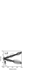
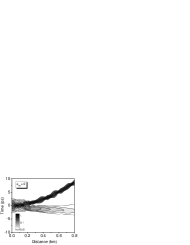
Figure 1: Simulation of breather splitting into the pulse pair. Contour plot of the field intensity. (a) Dispersion modulation phase is $\varphi_{m}=\pi$. (b) Dispersion modulation phase is $\varphi_{m}=0$. Energy of input pulse is 12.5 pJ. Width of initial pulse (7) is $T_{{}_{\rm FWHM}}=2.1\,\mbox{ps}$; Plots are normalized. Colorbar indicates the range of intensity values.

For dispersion modulation phase $\varphi_{m}=\pi$, only one modulation period of DOF ($z=0.16\,\mbox{km}$) is sufficient for the splitting of initial breather (Fig.1a). After $z=0.16\,\mbox{km}$ peak intensities of the pulses are reduced that leads to reduce of the effect of stimulated Raman scattering in further pulse propagation. For $\varphi_{m}=0$, the breather splits after propagation distance $z=0.24\,\mbox{km}$ (Fig.1b). Increased propagation distance of high-intensity breather leads to enhance effect of stimulated Raman scattering. As results the output pulses have very different peak intensities. Similar phenomena was observed experimentally [39].

Eigenvalues of solitons which form breather (7) are given by formula [7]

$$\lambda_{j}=i(N-j+1/2),$$ (9)

where $j=1,2,\dots$ and $j<(N+1/2)$. Imaginary part of the eigenvalue $Im(\lambda_{j})$ give soliton amplitude (2). Real part of the eigenvalue $Re(\lambda_{j})$ gives shift of the soliton carrier frequency (6). This spectral shift in turn shifts the pulse position in the time domain because of changes in the group velocity through fiber dispersion.

Eigenvalues (9) of initial solitons are purely imaginary. That means all solitons in breather (7) propagates with the same group velocity. The DOF changes soliton spectrum and real part of eigenvalues becomes nonzero. As result the solitons which form initial breather become separated in time. Figure 2a shows the change of peak to peak distance $\Delta T$ with increase of the energy of input pulse from 7.1 pJ to 12.5 pJ.

Eigenvalues of two solitons that arize due to the split of initial breather (7) in DOF are shown in Fig.2b. Curves in the Fig.2b were calculated by increase of the energy of input pulse. Directions of the movement of eigenvalues are shown by arrows. Starting points correspond to 7.1 pJ input pulse energy (soliton order is $N=1.65$). End points are marked by open circles and correspond to 12.5 pJ input pulse energy ($N=2.2$). Figure 2c shows that DOF can change $\lambda_{j}$ from purely imaginary values (9) at input to the values with distinct real part. The imaginary part of output solitons can be equalized by adjusting of input pulse energy.

(a)	(b)

Figure 2: Split of the breather in DOF. (a) Calculated peak to peak distance for output pulses. Open circle shows the point, which corresponds to experimental result with 12.5 pJ input pulse energy; (b) Movement of eigenvalues of output solitons with increase of the energy of input pulse from 7.1 pJ to 12.5 pJ. Arrows show the moving direction of the eigenvalues. Open circles corresponds to 12.5 pJ input pulse energy. The results were obtained for $\varphi_{m}=\pi$ Initial pulse width is $T_{{}_{\rm FWHM}}=2.1\,\mbox{ps}$.

In model of unperturbed NLSE the second-order breather ($N=2$) splits into solitons with eigenvalues which imaginary parts are equal and real parts are opposite in sign $Re(\lambda_{1})=-Re(\lambda_{2})$. This property follows from energy and momentum conservation laws [2, 3] for unperturbed Schrödinger equation. The main process that disturbs the splitting of the breather into two pulses with identical energies $Im(\lambda_{1})=Im(\lambda_{2})$ and opposite in sign frequency shift $Re(\lambda_{1})=-Re(\lambda_{2})$ is stimulated Raman scattering.

The results described above give optical all-fiber tool for the change of eigenvalues of picosecond solitons. The output pulses have different carrier frequencies that can be used to build up the high repetition rate multiwavelength optical clock.

4 Inelastic two-soliton interaction

Elastic collision of two solitons in case of ideal nonlinear Schrödinger equation results only in a shift of their phases and positions [2, 3]. However, even a relatively small perturbation changes this property. Under perturbation the solitons can change their velocities and amplitudes. In this section we describe inelastic soliton interactions forced by periodical variation of the fiber dispersion. As initial field a superposition of two single-soliton pulses was considered

$$A(0,t)=A_{0}\,{\rm sech}(t/t_{0}-T)+A_{0}\,{\rm sech}(t/t_{0}+T),$$ (10)

where $t_{0}=1.13$ ps is the initial pulse duration; $A_{0}=t_{0}^{-1}\left(|\langle\beta_{2}\rangle|/\langle\gamma\rangle\right)^{1/2}$ is the initial single-soliton pulse amplitude [3, 2]. The dimensionless parameter $T$ determines the separation between the peaks of the initial pulses. For the soliton pair (10) propagating in a constant-diameter fiber $(z_{m}=\infty)$ there exists an analytical solution [3, 11, 37]. In-phase solitons (10) periodically attract and repel. Period of oscillations is given by

$$z_{p}=2z_{0}(\lambda_{1}^{2}-\lambda_{2}^{2})^{-1},$$ (11)

where $z_{0}=0.158~{}\mbox{km}$ (8) is the soliton period [2, 3] in a constant diameter fiber $(z_{m}=\infty)$. Complex numbers $\lambda_{1}=i0.5(\sinh(T)-1)/\cosh(T)$ and $\lambda_{2}=i0.5(\sinh(T)+1)/\cosh(T)$ are soliton eigenvalues [37]. For non-interacting pulses $(T=\infty)$ the period of oscillations $z_{p}$ tends to infinity and soliton eigenvalues become equal $\lambda_{1}=\lambda_{2}=i0.5$. In the case of the NLSE with constant coefficients $(z_{m}=\infty)$, solitons interact elastically and their parameters $\lambda_{j}$ remain unchanged [3, 2, 6]. If there is dispersion modulation, interaction between solitons may have an inelastic nature, and the parameters $\lambda_{j}$ are variable.

The inelastic soliton collision in the Fig. 3 is shown. With initial pulse separation $T=6$ (fig.3ab) the initial soliton eigenvalues are $\lambda_{1}=i0.4975$ and $\lambda_{2}=i0.5025$. At initial stage of propagation in DOF, solitons are attracted (Fig.3a). And after collision they are repel. Due to the variation of the fiber dispersion, the collision of solitons occurs much earlier than predicted by the theory (11). The collision point is located at $z=18.83\,\mbox{km}$ (Fig. 3a). while analytical solution of unperturbed NLS equation (11) predicts the collision at $z_{c}=z_{p}/2=31.97\,\mbox{km}$. After collision, the solitons become propagating with the different group velocities (Fig.3a). Group velocity of soliton is associated with the shift of its carrier frequency $\Delta\Omega$ (6), which is defined by real part of soliton eigenvalue $Re(\lambda_{j})$.

(a)	(b)
(c)	(d)

Figure 3: Inelastic collision of two in-phase solitons in dispersion oscillating fiber (a,b) $T=6$; (c,d) $T=4$; (a,c), Contour plots of the field intensity $|A(z,t)|^{2}$; (b) Real part of eigenvalues vs. propagation distance. (d) Imaginary part of eigenvalues vs. propagation distance. Modulation period is $z_{m}=2.4\,\mbox{km}$, modulation phase is $\varphi_{m}=0$.

With initial pulse separation $T=4$ (3cd) the oscillation period is $z_{p}=8.66\,\mbox{km}$, initial soliton eigenvalues are $\lambda_{1}=i0.4814$ and $\lambda_{2}=i0.5180$. The soliton collision leads to the formation of central high-intensity pulse Fig. 3c. A part of radiation emerges into dispersive wave and goes out of the central pulse. The generation of the dispersive wave is forced by periodical perturbation of the dispersion [16]. Inverse scattering analysis show that inelastic collision leads to fusion of solitons and formation of two-soliton breather (Fig. 3d). The central frequencies of the solitons remains unchanged $(Re(\lambda_{j})=0)$. Figure 3 show that the DOF can be used to rearrange both the solitons carrier frequencies and the solitons energies. That reflects in the rearrangement of eigenvalues. The shift of carrier frequency of soliton is connected with the real part of its eigenvalue (6) and the soliton amplitude is given by imaginary part of the soliton eigenvalue (2).

At the considered parameters stimulated Raman scattering plays an important role in the distortion of the process of soliton collision. Figure 4 shows results of numerical solution of modified nonlinear Schrödinger equation (1) with $f_{R}=0.18$, $\alpha=0$, $\beta_{2}(z)$ and $\beta_{3}(z)$ are defined by (2).

(a)	(b)
(c)	(d)

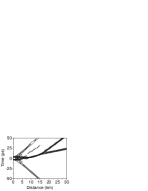
Figure 4: Inelastic collision of two in-phase solitons in presence of the stimulated Raman scattering and third-oder dispersion. (a), (b), $T=6.5$; (c), (d) $T=6$; (a), (c), Contour plots of the field intensity $|A(z,t)|^{2}$; (b), (d), Peak power. Modulation period is $z_{m}=847.5\,\mbox{m}$, modulation phase is $\varphi_{m}=0$.

The change of group velocities of two solitons (10) with initial pulse peak separation $T=6.5$ in the Fig. 4 is shown. The initial stage of pulses propagation is accompanied by the generation of the two dispersive waves which quickly goes out of the computation window. At the propagation distance $z=6.65\,\mbox{km}$ inelastic collision of initial pulses leads to formation of two solitons with different group velocities (Fig. 4a). The peak power of the resulting pulses decreases due to emergence of dispersive waves (Fig. 4b).

Variation of the time separation between initial solitons allows to control soliton dynamics. For $T=6$ (Fig. 4c) initial pulse merges into high-intensity breather at $z=7$ km. This breather propagates up to the distance $z=17$ km. The peak power of breather $(7~{}\mbox{km}<z<17~{}\mbox{km})$ is two times higher than the peak power of input pulses (Fig. 4d). After $z=17$ km the pulse decays into two low-intensity first-order solitons.

During propagation of first-order solitons, only a reduction in pulse energy due to the emission of a dispersive wave is possible. The dispersive wave has the highest intensity when the dispersion variation period coincides with the soliton period [16]. The period of dispersion variation $z_{m}$ does not coincide with the period of output first-order solitons (Fig. 4), so the energy loss due to the emission of a dispersive wave is a rather slow process. The high-intensity pulses (Fig. 4c) formed due to inelastic collisions of the solitons can propagate at the relative large propagation distances. However perturbation effects can lead to disappearance of high-intensity pulse. The solitons fusion and dynamics of high-intensity pulse can be considered as a birth and disappearance of rogue wave.

5 Discussion and outlook

Periodic modulation of the fiber diameter as a means of controlling soliton interaction and breather fission was proposed. We demonstrate all all-optical fiber technique for wavelength conversion between picosecond pulses based on splitting of optical breather into two pulses with different carrier frequencies and propagating with different group velocities. Our experiments showed clear dependence of the time distance between output pulses on the fiber modulation parameters, as predicted in theory. Splitting of the breather in dispersion oscillating fiber allows to build up pulse frequency division multiplexing from single picosecond laser source. Frequency division multiplexing of picosecond pulses can be used for high-speed multiwavelength optical clock for terabit hybrid WDM/TDM passive optical networks [38, 40]. The dispersion oscillating fiber can change eigenvalues that can be used for encoding channels in nonlinear frequency division multiplexing optical fiber networks [6].

References

- [1] N. N. Akhmediev and A. Ankiewicz, Solitons – Nonlinear Pulses and Beams, Chapman & Hall, New York, 1997.
- [2] G. P. Agrawal, Nonlinear Fiber Optics, Academic Press, San Diego, 2013 (5th edition).
- [3] S. A. Akhmanov, V. A. Vysloukh, and A. S.Chirkin, Optics of Femtosecond Laser Pulses, Am. Inst. of Physics, New York, 1992.
- [4] M. I. Yousefi, and F. R. Kschischang, “Information transmission using the nonlinear Fourier transform, Part I: Mathematical Tools,” IEEE Trans. on Inform. Theory 60, pp. 4312–4328, 2014.
- [5] S .K. Turitsyn, et al. “Nonlinear fourier transform for optical data processing and transmission: advances and perspectives,” Optica 4, pp. 307–322, 2017.
- [6] S. T. Le, V.Aref, and H. Buelow “Nonlinear signal multiplexing for communication beyond the Kerr nonlinearity limit,” Nature Photon. 11, pp. 570–576, (2017).
- [7] A. Hasegawa, and T. Nyu, “Eigenvalue communication,” J. of Lightwave Technol. 11, pp. 395–399, (1993).
- [8] A. Bendahmane, et al. “Dynamics of cascaded resonant radiations in a dispersion-varying optical fiber,” Optica 1, pp. 243–249, (2014).
- [9] G. Weerasekara, and A. Maruta, “Eigenvalue based analysis of soliton fusion phenomenon in the frame work of nonlinear Schrödinger equation,” IEEE Photonics Journal 9, pp 1–12, (2017).
- [10] I. S. Amiri, S. E. Alavi, and S. M. Idrus Soliton coding for secured optical communication link, Springer, Singapore, 2015.
- [11] R.-K. Lee, Y. Lai, and Y. S. Kivshar “Quantum correlations in soliton collisions,” Phys. Rev. A 71, p. 035801, 2005.
- [12] B. A. Malomed, Soliton Management in Periodic Systems, Springer, New York, 2006.
- [13] F. Reynaud, and A. Barthelemy, “Optically controlled interaction between two fundamental soliton beams”, Europhys. Lett. 12, pp. 401–405, 1990.
- [14] V. Tikhonenko, J. Christou, and B. Luther-Davies, “Three dimensional bright spatial soliton collision and fusion in a saturable nonlinear medium,” Phys. Rev. Lett. 76, pp. 2698–2701, 1996.
- [15] W. Królikowski, B. Luther-Davies, C. Denz, and T. Tschudi, “Annihilation of photorefractive solitons,” Opt. Lett. 23, pp. 97–99, 1998.
- [16] A. Hasegawa, and Y. Kodama “Guiding-center soliton,” Phys. Rev. Lett. 66, pp. 161–164, 1991.
- [17] D. Chao-Qing, and C. Wei-Lu, “Nonautonomous solitons in the continuous wave background of the variable-coefficient higher-order nonlinear Schrödinger equation,” Chinese Physics B 22, pp. 010507, 2013.
- [18] D. Mihalache, D. Mazilu, F. Lederer, and Yu. S. Kivshar, “Collisions between discrete surface spatiotemporal solitons in nonlinear waveguide arrays,” Phys. Rev. A 79, pp. 013811, 2009.
- [19] F. Lu, Q. Lin, W. H. Knox, and G. P. Agrawal, “Vector soliton fission,” Phys. Rev. Lett. 93, pp. 183901, 2004.
- [20] E. A. Golovchenko, E. M. Dianov, A. M. Prokhorov, and V. N. Serkin, “Decay of optical solitons,” JETP Lett. 42, pp. 87–91, 1985.
- [21] K. Tai, A. Hasegawa, and N. Bekki, “Fission of optical solitons induced by stimulated Raman effect,” Opt. Lett. 13, pp. 392–394, 1988.
- [22] S. Wang, X. Tang, and S. Lou, “Soliton fission and fusion: Burgers equation and Sharma-Tasso-Olver equation,” Chaos, Solitons, Fractals 21, pp. 231–239, 2004.
- [23] S. Gatz, and J. Herrmann, “Soliton collision and soliton fusion in dispersive linear and quadratic intensity refraction index change,” IEEE J. Quantum Electron. 28, pp. 1732–1738, 1992.
- [24] J. Pfeiffer, M. Schuster, A. A. Abdumalikov, Jr., and A. V. Ustinov, “Observation of soliton fusion in a Josephson array,” Phys. Rev. Lett. 96, pp. 034103, 2006.
- [25] W. Krolikowski, and S. A. Holmstrom, “Fusion and birth of spatial solitons upon collision,” Opt. Lett. 22, pp. 369–371, 1997.
- [26] S. R. Friberg, “Soliton fusion and steering by the simultaneous launch of two different-color solitons,” Opt. Lett. 16, pp. 1484–1486, 1991.
- [27] N. G. R. Broderick, “Method for pulse transformations using dispersion varying optical fiber tapers,” Opt. Expr. 18, pp. 24060–24069 (2010).
- [28] V. N. Serkin, and A. Hasegawa, “Soliton management in the nonlinear Schrödinger equation model with varying dispersion, nonlinearity, and gain,” Jour. of Exp. and Theor. Phys. Lett. 72, pp. 89–92, 2000.
- [29] C. H. Tenorio, et al. “Dynamics of solitons in the model of nonlinear Schrödinger equation with an external harmonic potential: I. Bright solitons,” Quant. Electron. 35, pp. 778–786, 2005.
- [30] Z. Yan, and C. Dai, “Optical rogue waves in the generalized inhomogeneous higher-order nonlinear Schrödinger equation with modulating coefficients,” J. of Opt. 15, pp. 064012, 2013.
- [31] D.-Y. Liu, B. Tian, and X.-Y. Xie, “Bound-state solitons for the coupled variable-coefficient higher-order nonlinear Schrödinger equations in the inhomogeneous optical fiber,” Laser Phys., 27, pp. 035403, 2017.
- [32] M. Onorato, D. Proment, “Triggering rogue waves in opposing currents,” Phys. Rev. Lett. 107, pp. 184502, 2011.
- [33] L. F. Mollenauer, and K. Smith, “Demonstration of soliton transmission over more than 4000 km in fiber with loss periodically compensated by Raman gain.” Opt. Lett. 13, pp. 675–677, 1988.
- [34] O. V. Sinkin, R. Holzlöhner, J. Zweck, and C. R. Menyuk, “Optimization of the split-step fourier method in modeling optical-fiber communications systems,” J. Lightwave Technol. 21, pp. 61–68, 2003.
- [35] A. I. Konyukhov et al., “On the all-fiber optical methods of the generation and recognition of soliton states,” J. of Exp. and Theor. Phys., V. 128, Issue 3, 2019, pp 384–395.
- [36] J.-C. Diels, W. Rudolph, Ultrashort Laser Pulse Phenomena, Academic Press, Boston, 2006 (2nd edition).
- [37] V. A. Vysloukh, and I. V. Cherednik, “On restricted N-soliton solutions of the nonlinear Schrödinger equation,” Theor. and Math. Phys. 71, pp. 346–351, 1987.
- [38] A. Tamini, and M. M. Kakhki, “Investigation of coherent multicarrier code division multiple access for optical access networks,” Advances in Computer Science : an International Journal 5, pp. 73–77, 2016.
- [39] A. A. Sysoliatin et al., “Soliton fission management by dispersion oscillating fiber,” Opt. Expr. 15, pp. 16302–16307, 2007.
- [40] E. Wong, “Next-generation broadband access networks and technologies,” Journ. of Lightwave Technol. 30, pp. 597-608, 2012.