Possible molecular states in $B^{(*)}B^{(*)}$ scatterings

Abstract

We present that, if unitarizing the $B^{(*)}B^{(*)}$ scattering amplitudes in the constituent interchange model, one can find two bound state poles for $(I_{tot},S_{tot})=(0,1)$ $BB^{*}$ and $B^{*}B^{*}$ system, which corresponds to two $I(J^{P})=0(1^{+})$ doubly bottomed molecular states. Furthermore, it is noticed that the virtual states in $(1,0)$ $BB$, $(1,1)$ $BB^{*}$, $(1,0)$ $B^{*}B^{*}$, and $(1,2)$ $B^{*}B^{*}$ systems could produce enhancements of the module squares of the scattering $T$-matrix just above the related thresholds, which might correspond to $I(J^{P})=1(0^{+})$, $1(1^{+})$, and $1(2^{+})$ doubly bottomed molecular states, respectively. The calculation may be helpful for searching for the doubly bottomed molecular state in future experiments.

I Introduction

Since the $X(3872)$ was observed by Belle in 2003 Choi et al. (2003), searches for exotic multiquark states beyond the conventional meson classifications have attracted intense attentions both from experimental and theoretical sides. In these years, many unconventional hidden-charm or hidden-beauty states have been observed, as reviewed in refs. Guo et al. (2018); Chen et al. (2016); Lebed et al. (2017). Some of these states run out of the predictions of the quark potential model and can not be described by the naive quark model. As a result, new configurations such as hadron molecules, tetraquark states, hybrid states, are utilized to understand these exotic states. Many of these states are regarded as belonging to the valence quark configuration $Q\bar{Q}q\bar{q}$ (where $Q$ denotes $c$ or $b$ quarks and $q$ denotes light quarks), which implies that QCD can form hadron states in an unconventional way Weinberg (2013).

After the observations of so many hidden-charmed or hidden-bottomed states, there arises a natural question whether there exist similar doubly-charmed or doubly-bottomed molecular states with valence quark configuration $Q\bar{q}Q\bar{q}$. Recently, LHCb reported the doubly charmed baryon state $\Xi_{cc}^{++}$ Aaij et al. (2017), which inspired Karliner and Rosner to predict a doubly bottomed tetraquark state to be about 215 MeV below the $B^{-}\bar{B}^{0*}$ threshold soon later Karliner and Rosner (2017), while Eichten and Quig predicted it to be 121 MeV below the $B^{-}\bar{B}^{0*}$ threshold Eichten and Quigg (2017). In fact, theoretical explorations of such doubly-heavy meson states have been carried on by several groups for a long time, as was reviewed in ref. Liu et al. (2019). In 1986, it was found that the $bb\bar{u}\bar{d}$ state could be bounded in a non-relativistic potential model Zouzou et al. (1986). In 1999, Barnes $et.\ al.$ found that the $I=0$ $BB^{*}$ channel could be attractive and form a $J^{P}=1^{+}$ bound state by solving the schrodinger equation of the $BB$, $BB^{*}$, and $B^{*}B^{*}$ systemsBarnes et al. (1999a). After that, different approaches to investigate the possibility of forming doubly bottomed or doubly charmed meson states are studied through tetraquark models Vijande et al. (2009); Ebert et al. (2007); Ming et al. (2008); Du et al. (2013); Luo et al. (2017); Yang et al. (2009); Feng et al. (2013); Mehen (2017); Richard et al. (2018); Cai and Cohen (2019), meson exchange modelsWang et al. (2019); Liu et al. (2014); Xu et al. (2019); Li et al. (2013), which usually calculate the binding energies by solving the Schr$\ddot{\mathrm{o}}$dinger Equation with the potentials obtained in such models. There are also some other calculations based on the QCD sum rulesWang and Yan (2018); Agaev et al. (2019) or using the Lattice simulationsMichael and Pennanen (1999); Detmold et al. (2007); Bicudo and Wagner (2013); Brown and Orginos (2012); Bicudo et al. (2015, 2016). These calculations basically paid their attentions to whether the bound states could be formed in the particular channels and the results in different calculations are not the same though most of them claim that there is a bound state in the $I=0$ $BB^{*}$ channel with very high possibility. However, there could be cases where the near threshold structure in the lineshape could be caused by a virtial state or by a combined effect of the virtual state and the threshold, when the virtual state is very close to the threshold. In fact, there are models claiming that the famous $X(3872)$ could be a virtual state just below the threshold. However, the method of solving the Schrödinger equation or using lattice calculations could only produce the bound state and would not give the virtual states. To study the possibility of the near threshold virtual states, one needs to have a nonperturbative scattering amplitude and annalytically continue it to the complex plane and study the pole structure of the amplitude.

In this paper, we just try to study the binding problem of $BB$, $BB^{*}$, $B^{*}B^{*}$ systems by investigating the existence of poles in the unitary meson-meson scattering matrix. As is well known, a bound state will appear as a pole of the partial-wave $S$ matrix below the threshold on the physical Riemann sheet, while a virtual state will appear as a pole below the threshold on the second Riemann sheet. The unitary amplitude is obtained using the K-matrix method by unitarization of a Born approximation of the amplitude. The valence quark interchange model by Barnes and Swanson is adopted to provide the Born approximation of the meson-meson scattering amplitude Barnes and Swanson (1992); Barnes et al. (1999a). Then, the unitarization of partial-wave amplitudes are derived and the poles of unitarized scattering amplitudes could be extracted by analytically continuing the energy to the complex plane. All the S-wave partial wave amplitudes of $BB$, $BB^{*}$, $B^{*}B^{*}$ scatterings are analyzed and related bound-state or virtual-state poles are searched for.

The paper is organized as follows: The Barnes-Swanson model is introduced and discussed in Section II. The K-matrix unitarization method for the partial wave Barnes-Swanson amplitude is derived in Section III. Numerical results and discussions are devoted in Section IV.

II The model

In the constituent interchange model developed by Barnes and Swanson Barnes and Swanson (1992); Barnes et al. (1999b), the meson-meson scattering amplitude is calculated by the (anti)quark-(anti)quark interactions by assuming the one-gluon-exchange (OGE) color Coulomb interaction, spin-spin interaction, and linear scalar confinement interaction. In the coordinate space, the effective interaction Hamiltonian is

$$H_{I}=\sum_{ij}[(\frac{\alpha_{s}}{r_{ij}}-\frac{8\pi\alpha_{s}}{3m_{i}m_{j}}\vec{S}_{i}\cdot\vec{S}_{j}\delta(\vec{r}_{ij})-\frac{3b}{4}r_{ij})\sum_{a}\mathcal{F}^{a}(i)\cdot\mathcal{F}^{a}(j)],$$ (1)

where $i,j$ represent valence quark or anti-quark in different initial hadrons. The color generator $\mathcal{F}^{a}=\lambda^{a}/2$ for quarks and $\mathcal{F}^{a}=-\lambda^{aT}/2$ for anti-quarks. Actually, to make the scheme consistent, the quark-quark interactions have also been used in determining the meson spectroscopy and their wave functions, so the model has a small free parameter space.

It is more convenient to construct the scattering amplitude in the momentum space. First, the meson state is defined by the mock state to represent its wave function as

$$|A(n,{}^{2S+1}L_{J,M})(\vec{P})\rangle= \sum_{M_{L},M_{S}}\langle LM_{L}SM_{S}|JM\rangle\int\mathrm{d}^{3}p\,\psi_{nLM_{L}}(\vec{p})\,\chi^{12}_{SM_{S}}\,\phi^{12}\,\omega^{12}$$

$$\times\Big{|}q_{1}\Big{(}\frac{m_{1}}{m_{1}+m_{2}}\vec{P}+\vec{p}\Big{)}\bar{q}_{2}\Big{(}\frac{m_{2}}{m_{1}+m_{2}}\vec{P}-\vec{p}\Big{)}\Big{\rangle},$$

$\chi^{12}$, $\phi^{12}$ and $\omega^{12}$ are the spin wavefunction, flavor wave function and the color wave function, respectively. $p_{1}$ ($p_{2}$) and $m_{1}$ ($m_{2}$) are the momentum and mass of the quark (anti-quark). $\vec{P}=\vec{p}_{1}+\vec{p}_{2}$ is the momentum of the center of mass, and $\vec{p}=\frac{m_{2}\vec{p}_{1}-m_{1}\vec{p}_{2}}{m_{1}+m_{2}}$ is the relative momentum. $\psi_{nLM_{L}}$ is the wave function for the meson, $n$ being the radial quantum number. The normalization is $\langle\vec{P}^{\prime},\lambda^{\prime}|\vec{P},\lambda\rangle=\delta_{\lambda\lambda^{\prime}}\delta(\vec{P}^{\prime}-\vec{P})$, where $\lambda$ represents the quantum numbers such as $nJM$ and particle species.

Then, at the lowest order the scattering amplitude for the process $AB\rightarrow CD$ is just the matrix element of interaction $H_{I}$ between the initial state $|A,B\rangle$ and the final $\langle C,D|$ which is formed just by rearrangements of the quarks(anti-quarks) in the initial states. Thus, the $S$ matrix can be written down as

$$S_{fi}=\delta_{fi}-2\pi i\delta(E_{f}-E_{i})\langle C,D|H_{I}|A,B\rangle$$ (2)

where $i,f$ denotes the initial and final states, and the matrix element is expressed as

$$\langle C,D|H_{I}|A,B\rangle=\delta^{3}(\vec{C}+\vec{D}-\vec{A}-\vec{B})\mathcal{M}_{fi}$$ (3)

where the $\vec{C}$ denotes the momentum of particle $C$, similarly for others. Since the Hamiltonian is the interaction between the constituent (anti-)quarks, the matrix element would be the integration of the product of the spatial wave functions of the (anti-)quarks in the mesons and the constituent (anti-)quark scattering amplitude. To the Born order of the (anti-)quark scattering amplitude, there are four kinds of $q\bar{q}-q\bar{q}$ scattering diagrams which are labeled according to which pairs of the constituents are interacted. These are $q$-$\bar{q}$ interaction diagrams, i.e. “capture₁” ($C_{1}$) and “capture₂” ($C_{2}$), and $q$-$q$ ($\bar{q}$-$\bar{q}$) interaction diagrams, i.e. “transfer₁” ($T_{1}$), and “transfer₂” ($T_{2}$), as shown in Fig. 1.

Figure 1: The four quark rearrangement diagrams of $AB\rightarrow CD$ meson-meson scatterings for anti-quark exchange. The arrows represent the quark line directions.

To evaluate the contributions of these diagrams, it is more convenient to redefine the momentum variables as in Fig. 2. In the $q_{a}(\bar{q}_{a})+q_{b}(\bar{q}_{b})\to q_{a^{\prime}}(\bar{q}_{a^{\prime}})+q_{b^{\prime}}(\bar{q}_{b^{\prime}})$ quark(antiquark) transitions, the initial and final momenta are denoted as $\vec{a}\vec{b}\to\vec{a}^{\prime}\vec{b}^{\prime}$. It is convenient to define $\vec{q}=\vec{a}^{\prime}-\vec{a}$, $\vec{p}=(\vec{a}^{\prime}+\vec{a})/2$.

Figure 2: Momentum redefinition in the quark-quark transition.

Then, the $T$-matrix element $\mathcal{M}_{fi}$ is contributed by the sum of all four kinds of diagrams, and the contribution of every diagram could be written down as the product of signature, flavor, color, spin, and space factors, represented as $h=I_{sign}I_{flavor}I_{color}I_{spin}I_{space}$. The signature factor is $(-1)$ for all diagrams because of interchanging three quark lines as shown in Fig.1. The color factor is $(-4/9)$ for two capture diagrams ($C_{1}$ and $C_{2}$) and $(4/9)$ for two transfer diagrams ($T_{1}$ and $T_{2}$). The spin factors for $C_{1}$, $C_{2}$, $T_{1}$, and $T_{2}$ diagrams in different interaction terms are listed in Table. 1.

Table 1: Compilation of the spin factors for $C_{1}$, $C_{2}$, $T_{1}$, and $T_{2}$ diagrams in the spin-spin hyperfine, color Coulomb, and linear potential terms Barnes and Swanson (1992).

$(S_{A},S_{B})\rightarrow(S_{C},S_{D})$	$(0,0)\rightarrow(0,0)$				$(1,0)\rightarrow(1,0)$				$(0,1)\rightarrow(0,1)$
	$C_{1}$	$C_{2}$	$T_{1}$	$T_{2}$	$C_{1}$	$C_{2}$	$T_{1}$	$T_{2}$	$C_{1}$	$C_{2}$	$T_{1}$	$T_{2}$
spin-spin	$-3/8$	$-3/8$	$3/8$	$3/8$	$1/8$	$-3/8$	$-1/8$	$3/8$	$-3/8$	$1/8$	$-1/8$	$3/8$
Coulomb	$1/2$				$1/2$				$1/2$
linear	$1/2$				$1/2$				$1/2$
$(S_{A},S_{B})\rightarrow(S_{C},S_{D})$	$(1,1)\rightarrow(1,1),\ S_{tot}=2$				$(1,1)\rightarrow(1,1),\ S_{tot}=1$				$(1,1)\rightarrow(1,1),\ S_{tot}=0$
	$C_{1}$	$C_{2}$	$T_{1}$	$T_{2}$	$C_{1}$	$C_{2}$	$T_{1}$	$T_{2}$	$C_{1}$	$C_{2}$	$T_{1}$	$T_{2}$
spin-spin	$1/4$	$1/4$	$1/4$	$1/4$	$0$	$0$	$-1/2$	$1/2$	$-1/8$	$-1/8$	$5/8$	$5/8$
Coulomb	$1$				$0$				$-1/2$
linear	$1$				$0$				$-1/2$

The space factor for each diagram is an overlap integral of the meson wave functions times the underlying quark transition amplitude $T^{pot}_{fi}$. The overlap integrals of wave functions could be written down explicitly as

$$I^{C_{1}}_{space} =(2\pi)^{-3}\int\mathrm{d}^{3}q\mathrm{d}^{3}p\Phi^{*}_{C}(\vec{p}+\frac{\vec{q}}{2}-\frac{1+\lambda}{2}\vec{C})\Phi^{*}_{D}(\vec{p}-\frac{\vec{q}}{2}-\vec{A}-\frac{1-\lambda}{2}\vec{C})$$

$$\times T^{pot}_{fi}(\vec{q})\Phi_{A}(\vec{p}-\frac{\vec{q}}{2}-\frac{1+\lambda}{2}\vec{A})\Phi_{B}(\vec{p}-\frac{\vec{q}}{2}-\frac{1-\lambda}{2}\vec{A}-\vec{C}),$$

$$I^{C_{2}}_{space} =(2\pi)^{-3}\int\mathrm{d}^{3}q\mathrm{d}^{3}p\Phi^{*}_{C}(-\vec{p}+\frac{\vec{q}}{2}+\vec{A}-\frac{1+\lambda}{2}\vec{C})\Phi^{*}_{D}(-\vec{p}-\frac{\vec{q}}{2}-\frac{1-\lambda}{2}\vec{C})$$

$$\times T^{pot}_{fi}(\vec{q})\Phi_{A}(-\vec{p}+\frac{\vec{q}}{2}+\frac{1-\lambda}{2}\vec{A})\Phi_{B}(-\vec{p}+\frac{\vec{q}}{2}+\frac{1+\lambda}{2}\vec{A}-\vec{C}),$$

$$I^{T_{1}}_{space} =(2\pi)^{-3}\int\mathrm{d}^{3}q\mathrm{d}^{3}p\Phi^{*}_{C}(\vec{p}+\frac{\vec{q}}{2}-\frac{1+\lambda}{2}\vec{C})\Phi^{*}_{D}(\vec{p}-\frac{\vec{q}}{2}-\vec{A}-\frac{1-\lambda}{2}\vec{C})$$

$$\times T^{pot}_{fi}(\vec{q})\Phi_{A}(\vec{p}-\frac{\vec{q}}{2}-\frac{1+\lambda}{2}\vec{A})\Phi_{B}(\vec{p}+\frac{\vec{q}}{2}-\frac{1-\lambda}{2}\vec{A}-\vec{C}),$$

$$I^{T_{2}}_{space} =(2\pi)^{-3}\int\mathrm{d}^{3}q\mathrm{d}^{3}p\Phi^{*}_{C}(-\vec{p}+\frac{\vec{q}}{2}+\vec{A}-\frac{1+\lambda}{2}\vec{C})\Phi^{*}_{D}(-\vec{p}-\frac{\vec{q}}{2}-\frac{1-\lambda}{2}\vec{C})$$

$$\times T^{pot}_{fi}(\vec{q})\Phi_{A}(-\vec{p}+\frac{\vec{q}}{2}+\frac{1-\lambda}{2}\vec{A})\Phi_{B}(-\vec{p}-\frac{\vec{q}}{2}+\frac{1+\lambda}{2}\vec{A}-\vec{C}).$$

The contributions to the quark-quark amplitude $T^{pot}_{fi}$ by spin-spin, color Coulomb, and Linear confinement interactions read as

$$T^{pot}_{fi}(\vec{q})=\left\{\begin{array}[]{cc}-\frac{8\pi\alpha_{s}}{3m_{1}m_{2}}[\vec{S}_{1}\cdot\vec{S}_{2}]&\mathrm{Spin-spin}\\ \frac{4\pi\alpha_{s}}{q^{2}}\mathbf{\textit{I}}&\mathrm{Coulomb}\\ \frac{6\pi b}{q^{4}}\mathbf{\textit{I}}&\mathrm{Linear}\end{array}\right.$$ (8)

We will deal with the scattering amplitudes of $BB$, $BB^{*}$, and $B^{*}B^{*}$ systems. For simplicity, the $u$ and $d$ quarks are assumed to have the same mass. To study the physically allowed system with a certain total isospin quantum number listed in Table.2, the phase convention of the $B$ and $\bar{B}$ meson isodoublets is chosen to be $\{|\bar{B}^{0}\rangle,|B^{-}\rangle\}=\{-|b\bar{d}\rangle,|b\bar{u}\rangle\}$ and $\{|B^{+}\rangle,|B^{0}\rangle\}=\{-|u\bar{b}\rangle,-|d\bar{b}\rangle\}$, and similar for the $B^{*}$ and $\bar{B}^{*}$ states. For isospin $I=0$ $BB$ system, $|I=0,I_{3}=0\rangle=-\frac{1}{\sqrt{2}}(|b\bar{d}\rangle|b\bar{u}\rangle-|b\bar{u}\rangle|b\bar{d}\rangle)$. For isospin $I=1$ $BB$ system, $|I=1,I_{3}=0\rangle=-\frac{1}{\sqrt{2}}(|b\bar{d}\rangle|b\bar{u}\rangle+|b\bar{u}\rangle|b\bar{d}\rangle)$.

Table 2: The physically allowed systems for $B^{(*)}B^{(*)}$.

system	Total isospin	Total spin
	$I_{tot}$	$\ \ S_{tot}=0\ \$	$\ \ S_{tot}=1\ \$	$\ \ S_{tot}=2\ \$
$BB$	1	even L
	0	odd L
$BB^{*}$	1		all L
	0		all L
$B^{*}B^{*}$	1	even L	odd L	even L
	0	odd L	even L	odd L

For $BB$ system, the scattering amplitude with the total isospin $I=0$ could be expressed explicitly as

$$\langle BB|T|BB\rangle_{I=0} = \frac{1}{2}(\langle b\bar{d}|\langle b\bar{u}|-\langle b\bar{u}|\langle b\bar{d}|)T(|b\bar{d}\rangle|b\bar{u}\rangle-|b\bar{u}\rangle|b\bar{d}\rangle)$$ (9)

$$= -\frac{1}{2}\langle b\bar{d}|\langle b\bar{u}|T|b\bar{u}\rangle|b\bar{d}\rangle-\frac{1}{2}\langle b\bar{u}|\langle b\bar{d}|T|b\bar{d}\rangle|b\bar{u}\rangle+\frac{1}{2}\langle b\bar{d}|\langle b\bar{u}|T|b\bar{d}\rangle|b\bar{u}\rangle+\frac{1}{2}\langle b\bar{u}|\langle b\bar{d}|T|b\bar{u}\rangle|b\bar{d}\rangle$$

$$= -T_{fi}(AB\to CD)+T_{fi}(AB\to DC).$$

The latter two terms of the second line in Eq.(9) are related to the “symmetrized diagrams” with the quark-line exchange rather than the anti-quark line exchange Barnes and Swanson (1992), which has the effects of interchanging the final $C$ and $D$ mesons. Including both kinds of diagrams also keeps the amplitudes for $BB$ scattering to be Bose-symmetric. Similarly, for $I=1$ $BB$ scattering, the amplitude could be also written down as

$$\langle BB|T|BB\rangle_{I=1}=T_{fi}(AB\to CD)+T_{fi}(AB\to DC).$$ (10)

The $B^{*}B^{*}$ scatterings are similar to the $BB$ scatterings, so there is no need to write the relations down explicitly.

For the $BB^{*}\to BB^{*}$ scatterings, when I=0, the scattering amplitude could be expressed as

$$\langle BB^{*}|T|BB^{*}\rangle_{I=0}=\frac{1}{2}[-\langle\bar{B}^{0}B^{-*}|T|B^{-}\bar{B}^{0*}\rangle-\langle B^{-}\bar{B}^{0*}|T|\bar{B}^{0}B^{-*}\rangle+\langle\bar{B}^{0}B^{-*}|T|\bar{B}^{0}B^{-*}\rangle+\langle B^{-}\bar{B}^{0*}|T|B^{-}\bar{B}^{0*}\rangle]$$

$$=-\langle\bar{B}^{0}B^{-*}|T|B^{-}\bar{B}^{0*}\rangle+\langle\bar{B}^{0}B^{-*}|T|\bar{B}^{0}B^{-*}\rangle.$$ (11)

When I=1, the scattering amplitude reads as

$$\langle BB^{*}|T|BB^{*}\rangle_{I=1}=\frac{1}{2}[\langle\bar{B}^{0}B^{-*}|T|\bar{B}^{0}B^{-*}\rangle+\langle B^{-}\bar{B}^{0*}|T|B^{-}\bar{B}^{0*}\rangle+\langle\bar{B}^{0}B^{-*}|T|B^{-}\bar{B}^{0*}\rangle+\langle B^{-}\bar{B}^{0*}|T|\bar{B}^{0}B^{-*}\rangle]$$

$$=\langle\bar{B}^{0}B^{-*}|T|B^{-}\bar{B}^{0*}\rangle+\langle\bar{B}^{0}B^{-*}|T|\bar{B}^{0}B^{-*}\rangle.$$ (12)

Since the incoming two mesons are not identical, there is no Bose symmetry in this scattering amplitude. One have to notice that the latter term $\langle\bar{B}^{0}B^{-*}|T|\bar{B}^{0}B^{-*}\rangle$, which is contributed by the diagrams with quark line interchanged, is not just the amplitude with the two final mesons interchanged in the first term.

III Partial wave decomposition and unitarization

In the previous section, we only calculated the lowest order scattering amplitude, which contains different partial wave component and does not satisfy the nonperturbative unitarity. Thus it needs partial wave decomposition and unitarization. Here we briefly describe the partial-wave decomposition and unitarity relation in our convention.

In general, consider the scattering process of $12\to 1^{\prime}2^{\prime}$, where all particle are massive. We use $\vec{k}$($k^{\prime}$) to denote the momentum of partical $1$ ($1^{\prime}$) in the initial(final) states in the center of mass system and $E_{1},E_{2}$ ($E_{1}^{\prime},E_{2}^{\prime}$) to denote the energies for the two initial (final) particles with the total energy $E=E_{1}+E_{2}$. The spins and the third components are denoted as $s_{1}$, $\sigma_{1}$ for particle 1 and so on. By using the convention of Weinberg (2005), the amplitude could be expanded in partial waves as

$$\mathcal{M}_{\vec{k}^{\prime}\sigma_{1}^{\prime},-\vec{k}^{\prime}\sigma_{2}^{\prime},\vec{k}\sigma_{1},-\vec{k}\sigma_{2}}=(|\vec{k}||\vec{k}^{\prime}|E_{1}E_{2}E_{1}^{\prime}E_{2}^{\prime}/EE^{\prime})^{-1/2}\sum_{j\sigma l^{\prime}m^{\prime}s^{\prime}\mu^{\prime}lms\mu}C_{s_{1}s_{2}}(s,\mu;\sigma_{1},\sigma_{2})C_{ls}(j,\sigma;m,\mu)$$

$$C_{s_{1}^{\prime}s_{2}^{\prime}}(s^{\prime},\mu^{\prime};\sigma_{1}^{\prime},\sigma_{2}^{\prime})C_{l^{\prime}s^{\prime}}(j,\sigma;m^{\prime},\mu^{\prime})Y_{l^{\prime}}^{m^{\prime}}(\hat{k}^{\prime})Y_{l}^{m*}(\hat{k})M^{j}_{l^{\prime}s^{\prime},ls}$$ (13)

If we only considered the spin-spin, color Coulomb, and linear confinement interactions here, the total orbital angular momentum and the total spin are conserved separately. The partial wave amplitude with total angular momentum $j$ will be

$$M^{j}_{ls,ls}=2\pi(|\vec{k}||\vec{k}^{\prime}|E_{1}E_{2}E_{1}^{\prime}E_{2}^{\prime}/EE^{\prime})^{1/2}\sum_{\sigma_{1}\sigma_{2}\sigma_{1}^{\prime}\sigma_{2}^{\prime}}C_{s_{1}s_{2}}(s,\mu;\sigma_{1},\sigma_{2})$$

$$\times C_{s_{1}^{\prime}s_{2}^{\prime}}(s,\mu;\sigma_{1}^{\prime},\sigma_{2}^{\prime})\int\mathrm{d}\mathrm{cos}\tilde{\theta}P_{l}(\mathrm{cos}\tilde{\theta})\mathcal{M}_{\vec{k}^{\prime}\sigma_{1}^{\prime},-\vec{k}^{\prime}\sigma_{2}^{\prime},\vec{k}\sigma_{1},-\vec{k}\sigma_{2}}$$ (14)

where $\tilde{\theta}$ is the angle between $\vec{k}$ and $\vec{k}^{\prime}$. That means, in this calculation, the partial-wave elastic unitarity condition is as simple as that of the scalar particles

$$\mathrm{Im}[M^{j}_{ls}]=\pi M^{j*}_{ls}M^{j}_{ls},$$ (15)

where we have omitted the repeated subscript $ls$ for brevity and $\mathrm{Im}[\ \ ]$ means the imaginary part of the related function. If we redefine the amplitude $M^{j}_{ls}=\frac{1}{\pi}\rho t_{l}$ by extracting the kinematic factor $\rho=\frac{2|\vec{k}|}{E}$, one will obtain a familiar form similar to the elastic unitarity condition of partial waves for scalar particles as

$$\mathrm{Im}[t_{l}]=\rho t_{l}^{*}t_{l}$$ (16)

or in a more concise form

$$\mathrm{Im}[t_{l}^{-1}]=-\rho.$$ (17)

In the constituent interchange model, only the Born term is calculated, so there is no elastic cut in the scattering amplitude and it does not obey the unitarity relation. One need to restore it by adopting a suitable unitarization scheme. Here we use the K-matrix unitarization method, which could be regarded as summing over all the bubble chains. Then, the unitarized partial-wave $S$ matrix element could be represented as

$$S_{l}=1+2iT=\frac{1+i\rho t_{l}}{1-i\rho t_{l}},$$ (18)

and the scattering $T$-matrix element is

$$T_{l}=\frac{\rho t_{l}}{1-i\rho t_{l}}.$$ (19)

The pole of $S$-matrix element below the threshold on the real axis of the first Riemann sheet, satisfying $1-i\rho t_{l}=0$, represents a bound state. When the unitarity relation is satisfied, the scatteing $S$-matrix on the second Riemann sheet is the inverse of that on the first Riemann sheet, $S^{\mathrm{2nd\ sheet}}=1/S^{\mathrm{1st\ sheet}}$, that means, the zero point of the first Riemann sheet corresponds to the pole of the second sheet. Thus, the zero point satisfying $1+i\rho t_{l}=0$ below the threshold represents a virtual state.

IV Numerical calculations and discussions

The parameters in the calculation is provided by the Godfrey-Isgur (GI) model Godfrey and Isgur (1985) because its interactions are similar to those in the Barnes-Swanson model and it presented a generally successful prediction to the meson mass spectrum. In the GI model, the wave functions of mesons are expanded in a series of a very large number of harmonics oscillator (HO) wave functions, which make it difficult to decompose the amplitude in the angular momentum in an analytical form, so we approximate the meson wave function by a HO wave function carrying the same radial quantum number and orbital angular momentum as the meson, with its effective radius obtained by the rms radius $r_{rms}$ of the related meson state in the GI model.

The running coupling function is parameterized as $\alpha_{s}(q^{2})=0.25e^{-q^{2}}+0.15e^{-\frac{q^{2}}{10}}+0.20e^{-\frac{q^{2}}{1000}}$ to saturate the result of perturbation theory calculation in the large $q^{2}$ region and avoid the divergence in the low $q^{2}$ region, and the quark masses used here are $m_{u}=m_{d}=0.22$GeV, $m_{b}=4.977$GeV. The strength coefficient of the confinement linear potential is $b=0.18$. We used the HO wave functions, with the oscillator parameters of the bottomed mesons as $\beta_{B}=0.579$GeV, $\beta_{B^{*}}=0.542$GeV ($\beta$ is defined in the HO wave function by $\psi(\vec{r})\sim(\mathrm{polynomial})\times e^{-\beta^{2}r^{2}/2}$).

In this calculation, only the partial $S$-wave scatterings of $B^{(*)}B^{(*)}$ are investigated. The scattering systems are labeled by their total isospins and total spins as $(I_{tot},S_{tot})$. Thus, the $B^{(*)}B^{(*)}$ systems discussed here, which could have non-vanishing partial $S$-waves, are $(1,0)$ $BB$, $(1,1)$ $BB^{*}$, $(0,1)$ $BB^{*}$, $(1,0)$ $B^{*}B^{*}$, $(0,1)$ $B^{*}B^{*}$, $(1,2)$ $B^{*}B^{*}$, as listed in Table. 2. Using the standard parameters listed above, there are a bound state found in $(0,1)$ $BB^{*}$ system and $(0,1)$ $B^{*}B^{*}$ system respectively, and one virtual pole is found in each of the other systems, whose pole positions are listed in Table.3. All the bound states and virtual states are just near the thresholds of the related channels.

Usually, if there is a virtual state close enough to the threshold, it will produce an enhancement for the absolute square of the scattering amplitude $|T|^{2}$ just above the related thresholds, which could be discerned in experiments. Whether the threshold enhancement could be recogonized as a state also depends on the interplay between the wave functions and the threshold. As shown in Fig.3, although there is a near threshold virtual state in each of the $(1,0)$ $BB$, $(1,1)$ $BB^{*}$, $(1,0)$ $B^{*}B^{*}$, and $(1,2)$ $B^{*}B^{*}$ systems, the near threshold peaks of $|T|^{2}$ in $(1,1)$ $BB^{*}$ and $(1,2)$ $B^{*}B^{*}$ systems are more obvious than the other two even though the virtuals states in the latter are closer to the related thresholds than the former.

In Ref. Barnes et al. (1999b), the authors extracted approximated local potentials from a part of the Born amplitudes which are calculated using the BS model. Then by solving the two-meson schrodinger equation with these potentials, they found that only the $I=0$ $BB^{*}$ channel is attractive enough to form a $I(J^{P})=0(1^{+})$ bound state with a binding energy of $-5.5$ MeV, which is consistent with our result. We also found that the $(0,1)$ $B^{*}B^{*}$ system could also form another $I(J^{P})=0(1^{+})$ bound state. Since our unitarization approach is using the full Born amplitude and the wave functions and coupling function used in the calculation are also different from the method In Ref. Barnes et al. (1999b), the differences between the results may not be surprising. In addition, our method provide more informations about the appearance of the virtual states. Another approach using the heavy meson chiral effective theory in Ref. Wang et al. (2019) also found that the $I(J^{P})=0(1^{+})$ $BB^{*}$ and $B^{*}B^{*}$ systems are attractive and obtain two bound states with their binding energies to be $\Delta E_{BB^{*}}\sim-12.6^{+9.2}_{-12.9}$ MeV and $\Delta E_{B^{*}B^{*}}\sim-23.8^{+16.3}_{-21.5}$ MeV, respectively. This may indicate a strong interaction in both of the $(0,1)$ $BB^{*}$ and the $(0,1)$ $B^{*}B^{*}$ system, which is similar in our result.

Table 3: The pole positions of the physically allowed systems for $B^{(*)}B^{(*)}$. The subscript “$v$” denotes a virtual state and “$b$” a bound state.

system(threshold)	Total isospin	Total spin
	$I_{tot}$	$\ \ S_{tot}=0\ \$	$\ \ S_{tot}=1\ \$	$\ \ S_{tot}=2\ \$
$BB$	1	$E_{v}=10557.8$MeV
($E_{th}=10558.6$MeV)	0
$BB^{*}$	1		$E_{v}=10600.6$MeV
($E_{th}=10604.0$MeV)	0		$E_{b}=10600.9$MeV
$B^{*}B^{*}$	1	$E_{v}=10648.7$MeV		$E_{v}=10648.3$MeV
($E_{th}=10649.4$MeV)	0		$E_{b}=10648.6$MeV

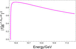
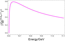
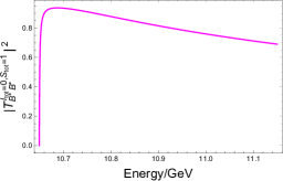
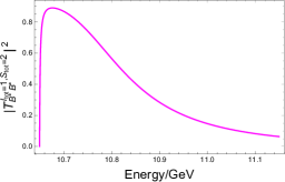
Figure 3: The absolute squares of scattering $T$-matrix of $(I_{tot},S_{tot})=(1,0)$ $BB$, $(1,1)$ $BB^{*}$, $(0,1)$ $BB^{*}$, $(1,0)$ $B^{*}B^{*}$, $(0,1)$ $B^{*}B^{*}$, and $(1,2)$ $B^{*}B^{*}$ systems.

There is a simple qualitative argument for the appearance of the virtual states in different channels in our calculation. We have stated that the virtual state would produce a near threshold enhancement in the $|T|^{2}$ to be observed in the experiments, which means that there is a large scattering length in these processes. In fact, from the theoretical point of view, it is the large scattering length calculated from BS model that causes the existence of the virtual states. In the K-matrix formalism, the virtual state pole position is the solution to $1+i\rho t_{l}=0$. If the perturbative scattering amplitude $t_{l}$ at the threshold, which is just proportional to the scattering length, is positive and large enough, $1+i\rho t_{l}=0$ will be saturated near the threshold, because the kinematic factor $i\rho$ is negative below the threshold and approaches to zero at the threshold. We can also see that the larger the scattering length is, the nearer the position of solution is to the threshold. Because of the large scattering length, $|T|^{2}$ will usually present a peak just above the threshold, which is observed in the experiments as a state. Similarly, if $t_{l}$ is negative and its absolute value is large, it will imply a near-threshold bound state. But for the deep bound state, it will depend on the detailed behavior of $t_{l}$ below the threshold. Thus, in general, as long as a model can produce a scattering length with a large enough absolute value, there would be a near-threshold virtual state or bound state generated. Thus, it is the large absolute values of the scattering lengths calculated from the BS model in these systems, as shown in Table 4, that are essential for the presence of the near threshold virtual and bound states. Since BS model is a nonrelativistic model, we would expect that the near threshold property, in particular the largeness of the scattering length, is qualitatively correct. Thus the appearance of the near threshold virtual states might be a more general result.

Table 4: The scattering lengthes of different $B^{(*)}B^{(*)}$ scatterings. Unit is $\mathrm{GeV}^{-1}$.

system(threshold)	Total isospin	Total spin
	$I_{tot}$	$\ \ S_{tot}=0\ \$	$\ \ S_{tot}=1\ \$	$\ \ S_{tot}=2\ \$
$BB$	1	14.8
($E_{th}=10558.6$MeV)	0
$BB^{*}$	1		7.01
($E_{th}=10604.0$MeV)	0		-7.39
$B^{*}B^{*}$	1	16.3		12.8
($E_{th}=10649.4$MeV)	0		-15.0

A further remark about the two $I(J^{P})=0(1^{+})$ states generated in $BB^{*}$ and $B^{*}B^{*}$ systems is in order. Since only the $S$-wave amplitudes are considered in our calculation and different systems are decoupled, the two states in $(I_{tot}=0,S_{tot}=1)$ $BB^{*}$ and $B^{*}B^{*}$ actually have the same quantum numbers but are different states. If these two channels are coupled to each other in reality, they could appear in both channels and may affect each other.

V Summary

In this paper, we use the Barnes-Swanson constituent interchange model to provide the Born term of $B^{(*)}B^{(*)}$ scattering amplitude and then unitarize them using the K-matrix method. By analytically continuing the unitarized scattering amplitudes to the complex energy plane, the dynamically generated bound states or virtual states could be extracted. Two bound states with $I(J^{P})=0(1^{+})$ are found at about 10600.9 MeV in $BB^{*}$ scattering and at about 10648.6 MeV in $B^{*}B^{*}$ scattering, respectively. We also found that several near threshold virtual states could be found in $(1,0)$ $BB$, $(1,1)$ $BB^{*}$, $(1,0)$ $B^{*}B^{*}$, and $(1,2)$ $B^{*}B^{*}$ systems, which might produce threshold enhancements and correspond to doubly bottomed molecular states.

In comparison, the other methods used in discussing the states in these systems, such as solving the schrödinger equation Barnes et al. (1999b) using the potentials extracted from the amplitude, or the heavy meson chiral effective theory discussion Wang et al. (2019), could only produce the near threshold bound state information and can not say anything about virtual states. Besides the bound states, our method also predicts the near-threshold virtual states in these systems which may have observable effects and could also inspire more interests in searching for threshold enhancements in experimental explorations. We also provide a simple qualitative explanation that it is the large scattering length calculated from the BS model that is essential in generating these virtual states which may be a more general result. From these different approaches, we expect that the existence of the near threshold composite states may be a general result in the $S$-wave $BB$, $BB^{*}$ and $B^{*}B^{*}$ systems.