Matias D. Cattaneo
Princeton University
Princeton, NJ
cattaneo@princeton.edu
and Rocio Titiunik
Princeton University
Princeton, NJ
titiunik@princeton.edu
and Gonzalo Vazquez-Bare
UC Santa Barbara
Santa Barbara, CA
gvazquez@econ.ucsb.edu
Analysis of Regression Discontinuity Designs with Multiple Cutoffs or Multiple Scores
Abstract
We introduce the Stata (and R) package rdmulti, which includes three commands (rdmc, rdmcplot, rdms) for analyzing Regression Discontinuity (RD) designs with multiple cutoffs or multiple scores. The command rdmc applies to non-cumulative and cumulative multi-cutoff RD settings. It calculates pooled and cutoff-specific RD treatment effects, and provides robust bias-corrected inference procedures. Post estimation and inference is allowed. The command rdmcplot offers RD plots for multi-cutoff settings. Finally, the command rdms concerns multi-score settings, covering in particular cumulative cutoffs and two running variables contexts. It also calculates pooled and cutoff-specific RD treatment effects, provides robust bias-corrected inference procedures, and allows for post-estimation estimation and inference. These commands employ the Stata (and R) package rdrobust for plotting, estimation, and inference. Companion R functions with the same syntax and capabilities are provided.
keywords:
st0001, regression discontinuity designs, multiple cutoffs, multiple scores, local polynomial methods.This version:
1 Introduction
Regression discontinuity (RD) designs with multiple cutoffs or multiple scores are commonly encountered in empirical work in Economics, Education, Political Science, Public Policy, and many other disciplines. As a consequence, these specific settings have also received attention in the recent RD methodological literature (Papay, Willett, and Murnane, 2011; Reardon and Robinson, 2012; Wong, Steiner, and Cook, 2013; Keele and Titiunik, 2015; Keele, Titiunik, and Zubizarreta, 2015; Cattaneo, Keele, Titiunik, and Vazquez-Bare, 2016a, 2021, and references therein). In this article, we introduce the software package rdmulti, which includes three Stata commands (and analogous R functions) for the analysis of RD designs with multiple cutoffs or multiple scores.
The command rdmc applies to non-cumulative and cumulative multi-cutoff RD settings, following recent work in Cattaneo, Keele, Titiunik, and Vazquez-Bare (2016a, 2021). Specifically, it calculates pooled and cutoff-specific RD treatment effects, employing local polynomial estimation and robust bias-corrected inference procedures. Post estimation and inference is allowed. The companion command rdmcplot offers RD plots for multi-cutoff settings. Finally, the command rdms concerns multi-score settings, covering in particular cumulative cutoffs and bivariate score contexts. It also calculates pooled and cutoff-specific RD treatment effects based on local polynomial methods, and allows for post-estimation estimation and inference. These commands employ the Stata (and R) package rdrobust for plotting, estimation, and inference; see Calonico, Cattaneo, and Titiunik (2014a, 2015b, 2017) for software details. See also Cattaneo, Titiunik, and Vazquez-Bare (2017) for a comparison of RD methodologies, Cattaneo, Idrobo, and Titiunik (2019a, 2020) and Cattaneo, Titiunik, and Vazquez-Bare (2019b) for a practical introductions to RD designs, and Cattaneo and Escanciano (2017) for a recent edited volume with further references.
To streamline the presentation, this article employs only simulated data to showcase all three settings covered by the package rdmulti: non-cumulative multiple cutoffs, cumulative multiple cutoffs, and bivariate score settings. For further discussion and illustration employing real data sets see Cattaneo, Idrobo, and
Titiunik (2020). The three settings covered by the package correspond, respectively, to (i) RD designs where different subgroups in the data are exposed to distinct but only one of the cutoff points (non-cumulative case), (ii) RD designs where units receive one single score and units are confronted to a sequence of ordered cutoffs points (cumulative case), and (iii) RD designs where units received two scores and there is a boundary on the plane determining the control and treatment areas. Well-known examples of each of these settings are:
Non-Cumulative Multiple Cutoffs: units in different groups (e.g., schools) receive an univariate score (e.g., test score) but the RD cutoff varies by group;
Cumulative Multiple Cutoffs: units receive the an univariate score (e.g., age) but different treatments are assigned at distinct score levels (e.g., at age 60 and at age 65);
Multiple Scores: units receive two scores (e.g., latitude and longitude) and treatment is assigned based on a boundary depending on both scores (e.g., geographic boundary).
We elaborate further on these cases in the upcoming sections, where we also give graphical representations of each case.
The Stata (and R) package rdmulti complements several recent software packages for RD designs. First, it explicitly relies on rdrobust (Calonico, Cattaneo, and Titiunik, 2014a, 2015b, 2017) for implementation, and hence further extends its scope to the case of RD designs with multiple cutoffs or multiple scores. Second, while the package focuses on local polynomial methods, related methods employing local randomization ideas and implemented in the package rdlocrand can also be used in the contexts of multiple cutoffs and multiple scores (Cattaneo, Titiunik, and Vazquez-Bare, 2016b). Third, the package rddensity (Cattaneo, Jansson, and Ma, 2018) can also be used in multiple cutoffs or multiple scores settings for falsification purposes. Finally, see the package rdpower (Cattaneo, Titiunik, and Vazquez-Bare, 2019c) for power calculations and sampling design methods, which can also be applied in the contexts discussed in this article.
The rest of the article is organized as follows. Section 2 gives a brief overview of the methods implemented in the package rdmulti, and also provides further references. Sections 3, 4 and 5 discuss the syntax of the commands rdmc, rdmcplot and rdms, respectively. Section 6 gives numerical illustrations, and Section 7 concludes. The latest version of this software, as well other software and materials useful for the analysis of RD designs, can be found at:
2 Overview of Methods
In this section we briefly describe the main ideas and methods used in the package rdmulti. For further methodological details see Keele and Titiunik (2015), Cattaneo, Keele, Titiunik, and Vazquez-Bare (2016a, 2021), Cattaneo, Idrobo, and Titiunik (2020), and references therein. All estimation and inference procedures employ rdplots (Calonico, Cattaneo, and Titiunik, 2015a) as well as local polynomial point estimation and robust bias correction inference methods (Calonico, Cattaneo, and Titiunik, 2014b, 2018, 2019, 2020b, 2020a).
2.1 Non-cumulative Multiple Cutoffs
In this case, individuals have a running variable and a vector of potential outcomes . Each individual faces a cutoff with . For example, Chay et al. (2005) study the effect of a school improvement program introduced in 1990 by the Chilean government. In this program, low-performing schools received public funding to improve infrastructure and teacher training, among other things. Assignment to this program was based on a school-level measure of test scores falling below a cutoff, where the cutoff was different across Chile’s 13 administrative regions. In this example, indicates each school’s administrative region, since this determines the cutoff faced by each school.
Unlike in a standard single-cutoff RD design, is a random variable. In a sharp design, individuals are treated when their running variable exceeds their corresponding cutoff, . A key feature of this design is that the variable partitions the population, that is, each unit faces one and only one value of . As the notation suggests, the potential outcomes for each individual are the same regardless of the specific cutoff they are exposed to; see Cattaneo, Keele, Titiunik, and Vazquez-Bare (2016a, 2021) for more discussion. Finally, we only consider finite multiple cutoffs because this is the most natural setting for empirical work: in practice, continuous cutoff are discretized for estimation and inference, as discussed and illustrated below.
Under regularity conditions, which include smoothness of conditional expectations among other things (see aforementioned references for details), the cutoff-specific treatment effects, , are identified by:
| (1) |
The pooled RD estimate is obtained by recentering the running variable, , thus normalizing the cutoff at zero:
| (2) |
where
| (3) |
All these parameters can be readily estimated using local polynomial methods (see Cattaneo, Idrobo, and Titiunik, 2019a, for a practical introduction), conditioning on cutoffs when appropriate. In other words, RD methods can by applied to each cutoff separately, in addition to pooling the data. Therefore, the rdmulti package implements bandwidth selection, estimation and inference based on local polynomial methods using the rdrobust command, described in Calonico et al. (2014a, 2015b, 2017). Specifically, the command rdmc allows for multi-cutoffs RD designs.
For the pooled parameter , the weights are estimated using the fact that ; see Cattaneo, Keele, Titiunik, and Vazquez-Bare (2016a) for further details. Then, given a bandwidth ,
When not specified by the user, the rdmc command uses the bandwidth selected by rdrobust when estimating the pooled effect to estimate the weights.
2.2 Cumulative Multiple Cutoffs
In an RD setting with cumulative cutoffs, individuals receive different treatments (or different dosages of a treatment) for different ranges of the running variable. In such setting, individuals receive treatment 1 if , treatment 2 if , and so on, until the last treatment value at . For example, Brollo et al. (2013) examine the effect of federal transfers on political corruption in Brazilian municipalities. The amount of the federal transfer that municipalities receive depends on the municipality’s population, and changes discretely at specified cutoffs. For example, municipalities with population below 10,189 receive a certain amount, municipalities with population between 10,189 and 13,585 receive a larger amount, and so on.
Denote the values of these treatments as , so that the treatment variable is now . Under standard regularity conditions, we have:
Since, unlike the case with multiple non-cumulative cutoffs, the population is not partitioned, each observation can be used to estimate two different (but contiguous on the score dimension) treatment effects. For example, units receiving treatment dosage are used as “treated” (i.e. above the cutoff ) when estimating and as “controls” when estimating (i.e. below the cutoff ). As a result, cutoff-specific estimators may not be independent, although the dependence disappears asymptotically as long as the bandwidths around each cutoff decrease with the sample size. On the other hand, bandwidths can be chosen to be non-overlapping to ensure that observations are used only once.
Once the data has been assigned to each cutoff under analysis, local polynomial methods can also be applied cutoff by cutoff in the cumulative multiple cutoffs case. We illustrate this approach below; for further discussion see Cattaneo, Idrobo, and Titiunik (2020), and the references therein.
2.3 Multiple Scores
In a multi-score RD design, treatment is assigned based on multiple running variables and some function determining a treatment “region” or “area”. We focus on the case with two running variables, , which is by far the most common case in empirical work. This case occurs naturally when, for instance, a treatment is assigned based on scores in two different exams (such as language and mathematics). Matsudaira (2008) estimates the effect of a mandatory summer school program assigned to students who fail to score higher than a preset cutoff in both math and reading exams. Another common case of multiple running variables occurs when a treatment is assigned based or based on geographic location (e.g., latitude and longitude). Keele and Titiunik (2015) discuss the effect of political campaign advertising on voter turnout and political attitudes by comparing voters in adjacent media markets, which result in different levels of exposure to advertising.
This type of assignment defines a continuum of treatment effects over the boundary of the treatment region, denoted by . For instance, if treatment is assigned to students scoring below 50 in language and mathematics, the treatment boundary is . For each point , the treatment effect at that point is given by
and under regularity conditions,
where and denote the control and treatment areas, respectively, and is a metric.
Since estimating a whole curve of treatment effects may not be feasible in practice, it is common to define a set of boundary points of interest at which to estimate the RD treatment effects. In the previous example, for instance, three points of interest on the boundary determining treatment assignment could be . On the other hand, the pooled RD estimand requires defining some measure of distance to the cutoff, such as the perpendicular (Euclidean) distance. This distance can be seen as the recentered running variable , which allows defining the pooled estimand as in Equation 2.
3 rdmc syntax
This section describes the syntax of the command rdmc, which estimates the pooled and cutoff-specific RD effects using rdrobust.
3.1 Syntax
rdmc depvar runvar if in , cvar(cutoff_var) fuzzy(string)
derivvar(string) pooled_opt(string) verbose pvar(string)
qvar(string) hvar(string) hrightvar(string) bvar(string)
brightvar(string) rhovar(string) covsvar(string) covsdropvar(string)
kernelvar(string) weightsvar(string) bwselectvar(string)
scaleparvar(string) scaleregulvar(string) masspointsvar(string)
bwcheckvar(string) bwrestrictvar(string) stdvarsvar(string)
vcevar(string) level(#) plot graph_opt(string)
depvar is the dependent variable.
runvar is the running variable (a.k.a. score or forcing variable).
cvar(cutoff_var) specifies the numeric variable cutoff_var that indicates the cutoff faced by each unit in the sample.
fuzzy(string) indicates a fuzzy design. See help rdrobust for details.
derivvar(string) a variable of length equal to the number of different cutoffs that specifies the order of the derivative for rdrobust to calculate cutoff-specific estimates. See help rdrobust for details.
pooled_opt(string) specifies the options to be passed to rdrobust to calculate pooled estimate. See help rdrobust for details.
verbose displays the output from rdrobust to calculate pooled estimand.
pvar(string) a variable of length equal to the number of different cutoffs that specifies the order of the polynomials for rdrobust to calculate cutoff-specific estimates. See help rdrobust for details.
qvar(string) a variable of length equal to the number of different cutoffs that specifies the order of the polynomials for bias estimation for rdrobust to calculate cutoff-specific estimates. See help rdrobust for details.
hvar(string) a variable of length equal to the number of different cutoffs that specifies the bandwidths for rdrobust to calculate cutoff-specific estimates. When hrightvar is specified, hvar indicates the bandwidth to the left of the cutoff. When hrightvar is not specified, the same bandwidths are used at each side. See help rdrobust for details.
hrightvar(string) a variable of length equal to the number of different cutoffs that specifies the bandwidths to the right of the cutoff for rdrobust to calculate cutoff-specific estimates. When hrightvar is not specified, the same bandwidths in hvar are used at each side. See help rdrobust for details.
bvar(string) a variable of length equal to the number of different cutoffs that specifies the bandwidths for the bias for rdrobust to calculate cutoff-specific estimates. When brightvar is specified, bvar indicates the bandwidth to the left of the cutoff. When brightvar is not specified, the same bandwidths are used at each side. See help rdrobust for details.
brightvar(string) a variable of length equal to the number of different cutoffs that specifies the bandwidths to the right of the cutoff for rdrobust to calculate cutoff-specific estimates. When brightvar is not specified, the same bandwidths in bvar are used at each side. See help rdrobust for details.
rhovar(string) a variable of length equal to the number of different cutoffs that specifies the value of rho for rdrobust to calculate cutoff-specific estimates. See help rdrobust for details.
covsvar(string) a variable of length equal to the number of different cutoffs that specifies the covariates for rdrobust to calculate cutoff-specific estimates. See help rdrobust for details.
covsdropvar(string) a variable of length equal to the number of different cutoffs that specifies whether collinear covariates should be dropped. See help rdrobust for details.
kernelvar(string) a variable of length equal to the number of different cutoffs that specifies the kernels for rdrobust to calculate cutoff-specific estimates. See help rdrobust for details.
weightsvar(string) a variable of length equal to the number of different cutoffs that specifies the weights for rdrobust to calculate cutoff-specific estimates. See help rdrobust for details.
bwselectvar(string) a variable of length equal to the number of different cutoffs that specifies the bandwidth selection method for rdrobust to calculate cutoff-specific estimates. See help rdrobust for details.
scaleparvar(string) a variable of length equal to the number of different cutoffs that specifies the value of scalepar for rdrobust to calculate cutoff-specific estimates. See help rdrobust for details.
scaleregulvar(string) a variable of length equal to the number of different cutoffs that specifies the value of scaleregul for rdrobust to calculate cutoff-specific estimates. See help rdrobust for details.
masspointsvar(string) a variable of length equal to the number of different cutoffs that specifies how to handle repeated values in the running variable. See help rdrobust for details.
bwcheckvar(string) a variable of length equal to the number of different cutoffs that specifies the value of bwcheck. See help rdrobust for details.
bwrestrictvar(string) variable of length equal to the number of different cutoffs that specifies whether computed bandwidths are restricted to the range of runvar. See help rdrobust for details.
stdvarsvar(string) a variable of length equal to the number of different cutoffs that specifies whether depvar and runvar are standardized. See help rdrobust for details.
vcevar(string) a variable of length equal to the number of different cutoffs that specifies the variance-covariance matrix estimation method for rdrobust to calculate cutoff-specific estimates. See help rdrobust for details.
level(#) specifies the confidence levels for confidence intervals. See help rdrobust for details.
plot plots the pooled and cutoff-specific estimates and the weights given by the pooled estimate to each cutoff-specific estimate.
graph_opt(string) options to be passed to the graph when plot is specified.
4 rdmcplot syntax
This section describes the syntax of the command rdmcplot, which plots the regression functions for each of the groups facing each cutoff using rdplot.
4.1 Syntax
rdmcplot depvar runvar if in , cvar(cutoff_var) nbinsvar(string)
nbinsrightvar(string) binselectvar(string)
scalevar(string) scalerightvar(string) supportvar(string)
supportrightvar(string) pvar(string) hvar(string) hrightvar(string)
kernelvar(string) weightsvar(string) covsvar(string)
covsevalvar(string) covsdropvar(string) binsoptvar(string)
lineoptvar(string) xlineoptvar(string) ci(cilevel) nobins nopoly
noxline nodraw genvars
depvar is the dependent variable.
runvar is the running variable (a.k.a. score or forcing variable).
cvar(cutoff_var) specifies the numeric variable cutoff_var that indicates the cutoff faced by each unit in the sample.
nbinsvar(string) a variable of length equal to the number of different cutoffs that specifies the number of bins for rdplot. When nbinsrightvar is specified, nbinsvar indicates the number of bins to the left of the cutoff. When nbinsrightvar is not specified, the same number of bins is used at each side. See help rdplot for details.
nbinsrightvar(string) a variable of length equal to the number of different cutoffs that specifies the number of bins to the right of the cutoff for rdplot. When nbinsrightvar is not specified, the number of bins in nbinsvar used at each side. See help rdplot for details.
binselectvar(string) a variable of length equal to the number of different cutoffs that specifies the bin selection method for rdplot. See help rdplot for details.
scalevar(string) a variable of length equal to the number of different cutoffs that specifies the scale for rdplot. When scalerightvar is specified, scalevar indicates the scale to the left of the cutoff. When scalerightvar is not specified, the same scale is used at each side. See help rdplot for details.
scalerightvar(string) a variable of length equal to the number of different cutoffs that specifies the scale to the right of the cutoff for rdplot. When scalerightvar is not specified, the scale in scalevar is used at each side. See help rdplot for details.
supportvar(string) a variable of length equal to the number of different cutoffs that specifies the support for rdplot. When supportrightvar is specified, supportvar indicates the support to the left of the cutoff. When supportrightvar is not specified, the same support is used at each side. See help rdplot for details.
supportrightvar(string) a variable of length equal to the number of different cutoffs that specifies the support to the right of the cutoff for rdplot. When supportrightvar is not specified, the support in supportvar is used at each side. See help rdplot for details.
pvar(string) a variable of length equal to the number of different cutoffs that specifies the order of the polynomials for rdplot. See help rdplot for details.
hvar(string) a variable of length equal to the number of different cutoffs that specifies the bandwidths for rdplot. When hrightvar is specified, hvar indicates the bandwidth to the left of the cutoff. When hrightvar is not specified, the same bandwidth is used at each side. See help rdplot for details.
hrightvar(string) a variable of length equal to the number of different cutoffs that specifies the bandwidth to the right of the cutoff for rdplot. When hrightvar is not specified, the bandwidth in hvar is used at each side. See help rdplot for details.
kernelvar(string) a variable of length equal to the number of different cutoffs that specifies the kernels for rdplot. See help rdplot for details.
weightsvar(string) a variable of length equal to the number of different cutoffs that specifies the weights for rdplot. See help rdplot for details.
covsvar(string) a variable of length equal to the number of different cutoffs that specifies the covariates for rdplot. See help rdplot for details.
covsevalvar(string) a variable of length equal to the number of different cutoffs that specifies the evaluation points for additional covariates. See help rdplot for details.
covsdropvar(string) a variable of length equal to the number of different cutoffs that specifies whether collinear covariates should be dropped. See help rdplot for details.
binsoptvar(string) a variable of length equal to the number of different cutoffs that specifies options for the bins plots.
lineoptvar(string) a variable of length equal to the number of different cutoffs that specifies options for the polynomial plots.
xlineoptvar(string) a variable of length equal to the number of different cutoffs that specifies options for the vertical lines indicating the cutoffs.
ci(cilevel) adds confidence intervals of levelcilevel to the plot.
nobins omits the bins plot.
nopoly omits the polynomial curve plot.
noxline omits the vertical lines indicating the cutoffs.
nodraw omits the plot.
genvars generates variables to replicate plots by hand. Variable labels indicate the corresponding cutoff.
rdmcplot_hat_y_c predicted value of the outcome variable given by the global polynomial estimator in cutoff number c.
rdmcplot_mean_x_c sample mean of the running variable within the corresponding bin for each observation in cutoff number c.
rdmcplot_mean_y_c sample mean of the outcome variable within the corresponding bin for each observation in cutoff number c.
rdmcplot_ci_l_c lower end value of the confidence interval for the sample mean of the outcome variable within the corresponding bin for each observation in cutoff number c.
rdmcplot_ci_r_c upper end value of the confidence interval for the sample mean of the outcome variable within the corresponding bin for each observation in cutoff number c.
5 rdms syntax
This section describes the syntax of the command rdms, which analyzes RD designs with cumulative cutoffs or two running variables.
5.1 Syntax
rdms depvar runvar1 [runvar2 treatvar] if in , cvar(cutoff_var1
[cutoff_var2])
range(range1 [range2]) xnorm(string)
fuzzy(string) derivvar(string) pooled_opt(string) pvar(string)
qvar(string) hvar(string) hrightvar(string) bvar(string)
brightvar(string) rhovar(string) covsvar(string) covsdropvar(string)
kernelvar(string) weightsvar(string) bwselectvar(string)
scaleparvar(string) scaleregulvar(string) masspointsvar(string)
bwcheckvar(string) bwrestrictvar(string) stdvarsvar(string)
vcevar(string) level(#) plot graph_opt(string)
depvar is the dependent variable.
runvar1 is the running variable (a.k.a. score or forcing variable) in a cumulative cutoffs setting.
runvar2 if specified, is the second running variable (a.k.a. score or forcing variable) in a two-score setting.
treatvar if specified, is the treatment indicator in a two-score setting.
cvar(cutoff_var1 [cutoff_var2]) specifies the numeric variable cutoff_var1 that indicates the cutoff faced by each unit in the sample in a cumulative cutoff setting, or the two running variables cutoff_var1 and cutoff_var2 in a two-score RD design.
range(range1 [range2]) specifies the range of the running variable to be used for estimation around each cutoff. Specifying only one variable implies using the same range at each side of the cutoff.
xnorm(string) specifies the normalized running variable to estimate pooled effect.
fuzzy(string) indicates a fuzzy design. See help rdrobust for details.
derivvar(string) a variable of length equal to the number of different cutoffs that specifies the order of the derivative for rdrobust to calculate cutoff-specific estimates. See help rdrobust for details.
pooled_opt(string) specifies the options to be passed to rdrobust to calculate pooled estimate. See help rdrobust for details.
pvar(string) a variable of length equal to the number of different cutoffs that specifies the order of the polynomials for rdrobust to calculate cutoff-specific estimates. See help rdrobust for details.
qvar(string) a variable of length equal to the number of different cutoffs that specifies the order of the polynomials for bias estimation for rdrobust to calculate cutoff-specific estimates. See help rdrobust for details.
hvar(string) a variable of length equal to the number of different cutoffs that specifies the bandwidths for rdrobust to calculate cutoff-specific estimates. When hrightvar is specified, hvar indicates the bandwidth to the left of the cutoff. When hrightvar is not specified, the same bandwidths are used at each side. See help rdrobust for details.
hrightvar(string) a variable of length equal to the number of different cutoffs that specifies the bandwidths to the right of the cutoff for rdrobust to calculate cutoff-specific estimates. When hrightvar is not specified, the same bandwidths in hvar are used at each side. See help rdrobust for details.
bvar(string) a variable of length equal to the number of different cutoffs that specifies the bandwidths for the bias for rdrobust to calculate cutoff-specific estimates. When brightvar is specified, bvar indicates the bandwidth to the left of the cutoff. When brightvar is not specified, the same bandwidths are used at each side. See help rdrobust for details.
brightvar(string) a variable of length equal to the number of different cutoffs that specifies the bandwidths to the right of the cutoff for rdrobust to calculate cutoff-specific estimates. When brightvar is not specified, the same bandwidths in bvar are used at each side. See help rdrobust for details.
rhovar(string) a variable of length equal to the number of different cutoffs that specifies the value of rho for rdrobust to calculate cutoff-specific estimates. See help rdrobust for details.
covsvar(string) a variable of length equal to the number of different cutoffs that specifies the covariates for rdrobust to calculate cutoff-specific estimates. See help rdrobust for details.
covsdropvar(string) a variable of length equal to the number of different cutoffs that specifies whether collinear covariates should be dropped. See help rdrobust for details.
kernelvar(string) a variable of length equal to the number of different cutoffs that specifies the kernels for rdrobust to calculate cutoff-specific estimates. See help rdrobust for details.
weightsvar(string) a variable of length equal to the number of different cutoffs that specifies the weights for rdrobust to calculate cutoff-specific estimates. See help rdrobust for details.
bwselectvar(string) a variable of length equal to the number of different cutoffs that specifies the bandwidth selection method for rdrobust to calculate cutoff-specific estimates. See help rdrobust for details.
scaleparvar(string) a variable of length equal to the number of different cutoffs that specifies the value of scalepar for rdrobust to calculate cutoff-specific estimates. See help rdrobust for details.
scaleregulvar(string) a variable of length equal to the number of different cutoffs that specifies the value of scaleregul for rdrobust to calculate cutoff-specific estimates. See help rdrobust for details.
masspointsvar(string) a variable of length equal to the number of different cutoffs that specifies how to handle repeated values in the running variable. See help rdrobust for details.
bwcheckvar(string) a variable of length equal to the number of different cutoffs that specifies the value of bwcheck. See help rdrobust for details.
bwrestrictvar(string) variable of length equal to the number of different cutoffs that specifies whether computed bandwidths are restricted to the range of runvar. See help rdrobust for details.
stdvarsvar(string) a variable of length equal to the number of different cutoffs that specifies whether depvar and runvar are standardized. See help rdrobust for details.
vcevar(string) a variable of length equal to the number of different cutoffs that specifies the variance-covariance matrix estimation method for rdrobust to calculate cutoff-specific estimates. See help rdrobust for details.
level(#) specifies the confidence levels for confidence intervals. See help rdrobust for details.
plot plots the pooled and cutoff-specific estimates and the weights given by the pooled estimate to each cutoff-specific estimate.
graph_opt(string) options to be passed to the graph when plot is specified.
6 Illustration of Methods
6.1 Non-cumulative Multiple Cutoffs
We begin by illustrating rdmc using a simulated dataset, simdata_multic. In this dataset, y is the outcome variable, x is the running variable, c is a variable indicating the cutoff that each unit in the sample faces, and t is a treatment indicator, corresponding in this case to units with . As shown below, there are two different cutoffs, 33 and 66, each with the sample sample size.
-
. use simdata_multic, clear

. sum

    Variable          Obs        Mean    Std. Dev.       Min        Max

           c        2,000        49.5    16.50413         33         66
           x        2,000    50.79875    28.95934   .0184725   99.97507
           t        2,000        .516    .4998689          0          1
           y        2,000    1728.135    545.0856   540.0849   3015.232

. tab c

          c        Freq.     Percent        Cum.

         33        1,000       50.00       50.00
         66        1,000       50.00      100.00

      Total        2,000      100.00
The basic syntax for rdmc is the following:
-
. rdmc y x, c(c)


Cutoff-specific RD estimation with robust bias-corrected inference

      Cutoff     Coef.    P>|z|  [95% Conf. Int.]     hl     hr      Nh   Weight

          33   484.831    0.00    421.18  552.53    14.66  14.66    289    0.540
          66   297.981    0.00    220.35  362.27    11.95  11.95    246    0.460

    Weighted   398.915    0.00    348.74  445.14        .      .    535        .
      Pooled   436.400    0.00    179.34  676.63    13.68  13.68    550        .
The output shows the cutoff-specific estimate at each cutoff, together with the corresponding robust bias-corrected p-value, 95 percent robust confidence interval and sample size at each cutoff, and two “global” estimates. The first one is a weighted average of the cutoff specific estimates using the estimated weights described in Section 2. These estimated weights are shown in the last column. The second one is the pooled estimate obtained by normalizing the running variable. While these two estimators converge to the same population parameter, they can differ in finite samples as seen above. In this example, the effect is statistically significant at both cutoffs.
All the results in the above display are calculated using rdrobust. The user can specify options for rdrobust to calculate the pooled estimates using the option pooled_opt. For instance, the syntax below specifies a bandwidth of 20 and a local quadratic polynomial for the pooled estimand. By default, rdmc omits the output from rdrobust when estimating the effects. The output from the pooled effect estimation can be displayed using the option verbose, which we use below to show how the options are passed to rdrobust.
-
. rdmc y x, c(c) pooled_opt(h(20) p(2)) verbose

Sharp RD estimates using local polynomial regression.

      Cutoff c = 0   Left of c  Right of c            Number of obs =       2000
                                                       BW type       =     Manual
     Number of obs         968        1032            Kernel        = Triangular
Eff. Number of obs         409         416            VCE method    =         NN
    Order est. (p)           2           2
    Order bias (q)           3           3
       BW est. (h)      20.000      20.000
       BW bias (b)      20.000      20.000
         rho (h/b)       1.000       1.000

Outcome: y. Running variable: __000002.

            Method     Coef.    Std. Err.    z     P>|z|    [95% Conf. Interval]

      Conventional    437.04      129.8   3.3671   0.001    182.643      691.441
            Robust       -          -     3.0118   0.003    185.618      877.381


Cutoff-specific RD estimation with robust bias-corrected inference

      Cutoff     Coef.    P>|z|  [95% Conf. Int.]     hl     hr      Nh   Weight

          33   484.831    0.00    421.18  552.53    14.66  14.66    289    0.540
          66   297.981    0.00    220.35  362.27    11.95  11.95    246    0.460

    Weighted   398.915    0.00    348.74  445.14        .      .    535        .
      Pooled   437.042    0.00    185.62  877.38    20.00  20.00    825        .
The user can also modify the options for estimation in each specific cutoff. The following syntax shows how to manually change options for the cutoff-specific estimates by setting a bandwidth of 11 in the first cutoff and 10 in the second one.
-
. gen double h = 11 in 1
(1,999 missing values generated)

. replace h = 10 in 2
(1 real change made)

. rdmc y x, c(c) h(h)


Cutoff-specific RD estimation with robust bias-corrected inference

      Cutoff     Coef.    P>|z|  [95% Conf. Int.]     hl     hr      Nh   Weight

          33   495.429    0.00    368.13  563.21    11.00  11.00    207    0.498
          66   303.769    0.00    220.40  403.32    10.00  10.00    209    0.502

    Weighted   399.138    0.00    321.56  455.23        .      .    416        .
      Pooled   436.400    0.00    179.34  676.63    13.68  13.68    550        .
All the cutoff-specific options are passed in a similar fashion, defining a new variable of length equal to the number of cutoffs that indicates the options for each cutoff in its values. For instance, the following syntax indicates different bandwidth selection methods at each cutoff:
-
. gen bwselect = "msetwo" in 1
(1,999 missing values generated)

. replace bwselect = "certwo" in 2
(1 real change made)

. rdmc y x, c(c) bwselect(bwselect)


Cutoff-specific RD estimation with robust bias-corrected inference

      Cutoff     Coef.    P>|z|  [95% Conf. Int.]     hl     hr      Nh   Weight

          33   481.567    0.00    417.80  546.83    14.49  16.91    313    0.570
          66   298.726    0.00    227.42  367.21    14.74   7.95    236    0.430

    Weighted   402.969    0.00    355.30  450.28        .      .    549        .
      Pooled   436.400    0.00    179.34  676.63    13.68  13.68    550        .
The rdmc command saves the bias-corrected estimates and variances in the matrices e(b) and e(V), which allows for post-estimation testing using lincom or test. For instance, to test whether the effects at the two cutoffs are the same, type:
-
. rdmc y x, c(c)


Cutoff-specific RD estimation with robust bias-corrected inference

      Cutoff     Coef.    P>|z|  [95% Conf. Int.]     hl     hr      Nh   Weight

          33   484.831    0.00    421.18  552.53    14.66  14.66    289    0.540
          66   297.981    0.00    220.35  362.27    11.95  11.95    246    0.460

    Weighted   398.915    0.00    348.74  445.14        .      .    535        .
      Pooled   436.400    0.00    179.34  676.63    13.68  13.68    550        .


. matlist e(b)

                      c1         c2   weighted     pooled

          y1    486.8578   291.3082   396.9415   427.9832

. lincom c1-c2

 ( 1)  c1 - c2 = 0


                    Coef.   Std. Err.      z    P>|z|     [95% Conf. Interval]

         (1)     195.5496    49.3309     3.96   0.000     98.86279    292.2364
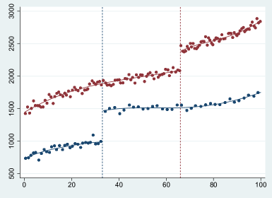
The rdmcplot command jointly plots the estimated regression functions at each cutoff. The output from rdmcplot is shown in Figure 1. The basic syntax is the following:
-
. rdmcplot y x, c(c)
The rdmcplot includes all the options available for rdplot. For example, the plot can be restricted to a bandwidth using the option h() and to use a polynomial of a specified order using the option p(), as shown below. This option allows the user to plot the linear fit and estimated treatment effects at each cutoff.
-
. gen p = 1 in 1/2
(1,998 missing values generated)

. rdmcplot y x, c(c) h(h) p(p)
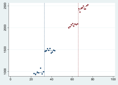
The resulting plot is shown in Figure 2.
The option genvars generates the variables required to replicate the plots by hand. This allows the user to customize the plot. The following code illustrates how to use this option to replicate Figure 2.
-
. rdmcplot y x, c(c) genvars

. twoway (scatter rdmcplot_mean_y_1 rdmcplot_mean_x_1, mcolor(navy)) ///
>         (line rdmcplot_hat_y_1 rdmcplot_mean_x_1 if t==1, sort lcolor(navy)) ///
>         (line rdmcplot_hat_y_1 rdmcplot_mean_x_1 if t==0, sort lcolor(navy)) ///
>         (scatter rdmcplot_mean_y_2 rdmcplot_mean_x_2, mcolor(maroon)) ///
>         (line rdmcplot_hat_y_2 rdmcplot_mean_x_2 if t==1, sort lcolor(maroon)) ///
>         (line rdmcplot_hat_y_2 rdmcplot_mean_x_2 if t==0, sort lcolor(maroon)), ///
>         xline(33, lcolor(navy) lpattern(dash)) ///
>         xline(66, lcolor(maroon) lpattern(dash)) ///
>         legend(off)
6.2 Cumulative Multiple Cutoffs
We now illustrate the use of rdms for cumulative cutoffs using the simulated dataset simdata_cumul. In this dataset, the running variable ranges from 0 to 100, and units with running variable below receive a certain treatment level whereas units with running variable above receive another treatment level . In this setting, the cutoffs are indicated as a variable in the dataset, where each row indicates a cutoff.
-
. use simdata_cumul, clear

. sum

    Variable          Obs        Mean    Std. Dev.       Min        Max

           x        1,000    50.46639    28.69369   .0413166    99.8783
           y        1,000    1508.638    488.2752   658.4198   2480.568
           c            2        49.5    23.33452         33         66

. tab c

          c        Freq.     Percent        Cum.

         33            1       50.00       50.00
         66            1       50.00      100.00

      Total            2      100.00
The syntax for cumulative cutoffs is similar to rdmc. The user specifies the outcome variable, the running variable and the cutoffs as follows:
-
. rdms y x, c(c)


Cutoff-specific RD estimation with robust bias-corrected inference

         Cutoff       Coef.     P>|z|     [95% Conf. Int.]     hl     hr      Nh

             33     395.492     0.000     363.76   423.86    15.11  15.11    286
             66     342.872     0.000     315.95   373.96    12.22  12.22    265
Options like the bandwidth, polynomial order and kernel for each cutoff-specific effect can be specified by creating variables as shown below.
-
. gen double h = 11 in 1
(999 missing values generated)

. replace h = 8 in 2
(1 real change made)

. gen kernel = "uniform" in 1
(999 missing values generated)

. replace kernel = "triangular" in 2
variable kernel was str7 now str10
(1 real change made)

. rdms y x, c(c) h(h) kernel(kernel)


Cutoff-specific RD estimation with robust bias-corrected inference

         Cutoff       Coef.     P>|z|     [95% Conf. Int.]     hl     hr      Nh

             33     394.470     0.000     351.65   438.72    11.00  11.00    215
             66     342.505     0.000     301.56   375.95     8.00   8.00    166
Without further information, the rdms command could be using any observation above the cutoff 33 to estimate the effect of the first treatment level . This implies that some observations in the range are used. But these observations receive the second treatment level, . This feature can result in inconsistent estimators for . To avoid this problem, the user can specify the range of observations to be used around each cutoff. In this case, we can restrict the range at the first cutoff (33) to go from 0 to 65.5, to ensure that no observations above 66 are used, and the range at the second cutoff (66) to go from 33.5 to 100. This can be done as follows.
-
. gen double range_l = 0 in 1
(999 missing values generated)

. gen double range_r = 65.5 in 1
(999 missing values generated)

. replace range_l = 33.5 in 2
(1 real change made)

. replace range_r = 100 in 2
(1 real change made)

. rdms y x, c(c) range(range_l range_r)


Cutoff-specific RD estimation with robust bias-corrected inference

         Cutoff       Coef.     P>|z|     [95% Conf. Int.]     hl     hr      Nh

             33     394.698     0.000     356.12   430.45    10.96  10.96    214
             66     342.180     0.000     312.20   372.04    11.18  11.18    246
The pooled estimate can be obtained using rdmc. For this, we need to assign each unit in the sample a value for the cutoff. One possibility is to assign each unit to the closest cutoff. For this, we generate a variable named cutoff that equals 33 for units with score below 49.5 (the middle point between 33 and 66), and equals 66 for units above 49.5.
-
. gen double cutoff = c[1]*(x<=49.5) + c[2]*(x>49.5)

. rdmc y x, c(cutoff)


Cutoff-specific RD estimation with robust bias-corrected inference

      Cutoff     Coef.    P>|z|  [95% Conf. Int.]     hl     hr      Nh   Weight

          33   389.528    0.00    332.94  443.69     6.26   6.26    119    0.531
          66   341.015    0.00    300.39  377.33     5.04   5.04    105    0.469

    Weighted   366.788    0.00    330.63  399.64        .      .    224        .
      Pooled   363.968    0.00    180.11  551.78     8.14   8.14    333        .
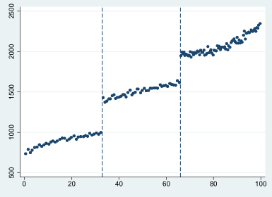
Finally, we can use the variable cutoff to plot the regression functions using rdmcplot, shown in Figure 3
-
. gen binsopt = "mcolor(navy)" in 1/2
(998 missing values generated)

. gen xlineopt = "lcolor(navy) lpattern(dash)" in 1/2
(998 missing values generated)

. rdmcplot y x, c(cutoff) binsoptvar(binsopt) xlineopt(xlineopt) nopoly
6.3 Multiple Scores
We now illustrate the use of rdms to analyze RD designs with two running variables using the simulated dataset simdata_multis. In this dataset, there are two running variables, x1 and x2, ranging between 0 and 100, and units receive the treatment when and . We look at three cutoffs on the boundary: (25,50), (50,50) and (50,25).
-
. use simdata_multis, clear

. sum

    Variable          Obs        Mean    Std. Dev.       Min        Max

          x1        1,000    50.22881    28.87868   .6323666   99.94879
          x2        1,000    50.63572     29.1905   .0775479   99.78458
           t        1,000        .223    .4164666          0          1
           y        1,000    728.5048    205.5627   329.4558   1372.777
          c1            3    41.66667    14.43376         25         50

          c2            3    41.66667    14.43376         25         50

. list c1 c2 in 1/3


       c1   c2

  1.   25   50
  2.   50   50
  3.   50   25
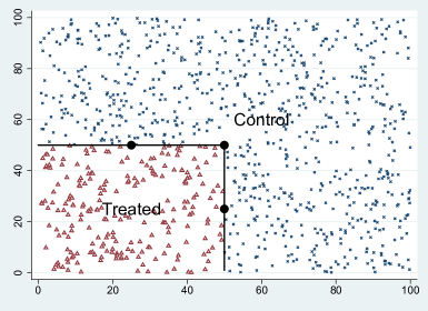
The following code provides a simple visualization of this setting, shown in Figure 4:
-
. gen xaux = 50 in 1/50
(950 missing values generated)

. gen yaux = _n in 1/50
(950 missing values generated)

. twoway (scatter x2 x1 if t==0, msize(small) mfcolor(white) msymbol(X)) ///
>            (scatter x2 x1 if t==1, msize(small) mfcolor(white) msymbol(T)) ///
>            (function y = 50, range(0 50) lcolor(black) lwidth(medthick)) ///
>            (line yaux xaux, lcolor(black) lwidth(medthick)) ///
>            (scatteri 50 25, msize(large) mcolor(black)) ///
>            (scatteri 50 50, msize(large) mcolor(black)) ///
>            (scatteri 25 50, msize(large) mcolor(black)), ///
>            text(25 25 "Treated", size(vlarge)) ///
>            text(60 60 "Control", size(vlarge)) ///
>            legend(off)
The basic syntax is the following:
-
. rdms y x1 x2 t, c(c1 c2)


Cutoff-specific RD estimation with robust bias-corrected inference

         Cutoff       Coef.     P>|z|     [95% Conf. Int.]     hl     hr      Nh

        (25,50)     243.842     0.111     -50.93   491.18    11.12  11.12     42
        (50,50)     578.691     0.000     410.83   764.88    13.83  13.83     47
        (50,25)     722.444     0.000     451.49  1060.15    10.83  10.83     38
Information to estimate each cutoff-specific estimate can be provided as illustrated before. For instance, to specify cutoff-specific bandwidths:
-
. gen double h = 15 in 1
(999 missing values generated)

. replace h = 13 in 2
(1 real change made)

. replace h = 17 in 3
(1 real change made)

. rdms y x1 x2 t, c(c1 c2) h(h)


Cutoff-specific RD estimation with robust bias-corrected inference

         Cutoff       Coef.     P>|z|     [95% Conf. Int.]     hl     hr      Nh

        (25,50)     336.121     0.233    -119.35   491.36    15.00  15.00     87
        (50,50)     583.047     0.000     501.94  1101.24    13.00  13.00     42
        (50,25)     620.692     0.000     464.92  1159.99    17.00  17.00     86
Finally, the xnorm option allows the user to specify the normalized running variable to calculate a pooled estimate. In this case, we define the normalized running variable as the closest perpendicular distance to the boundary defined by the treatment assignment, with positive values indicating treated units and negative values indicating control units.
-
. gen double aux1 = abs(50 - x1)

. gen double aux2 = abs(50 - x2)

. egen xnorm = rowmin(aux1 aux2)

. replace xnorm = xnorm*(2*t-1)
(777 real changes made)

. rdms y x1 x2 t, c(c1 c2) xnorm(xnorm)


Cutoff-specific RD estimation with robust bias-corrected inference

         Cutoff       Coef.     P>|z|     [95% Conf. Int.]     hl     hr      Nh

        (25,50)     243.842     0.111     -50.93   491.18    11.12  11.12     42
        (50,50)     578.691     0.000     410.83   764.88    13.83  13.83     47
        (50,25)     722.444     0.000     451.49  1060.15    10.83  10.83     38

         Pooled     447.017     0.000     389.33   496.85    12.73  12.73    433
7 Conclusion
We introduced the Stata package rdmulti to anlyze RD designs with multiple cutoffs or scores. A companion R function with the same syntax and capabilities is also provided.
8 Acknowledgments
We thank Sebastian Calonico and Nicolas Idrobo for helpful comments and discussions. The authors gratefully acknowledge financial support from the National Science Foundation through grant SES-1357561.
References
- Brollo et al. (2013) Brollo, F., T. Nannicini, R. Perotti, and G. Tabellini. 2013. The Political Resource Curse. American Economic Review 103(5): 1759–96.
- Calonico et al. (2018) Calonico, S., M. D. Cattaneo, and M. H. Farrell. 2018. On the Effect of Bias Estimation on Coverage Accuracy in Nonparametric Inference. Journal of the American Statistical Association 113(522): 767–779.
- Calonico et al. (2020a) ———. 2020a. Coverage Error Optimal Confidence Intervals for Local Polynomial Regression. arXiv:1808.01398 .
- Calonico et al. (2020b) ———. 2020b. Optimal Bandwidth Choice for Robust Bias Corrected Inference in Regression Discontinuity Designs. Econometrics Journal, forthcoming .
- Calonico et al. (2017) Calonico, S., M. D. Cattaneo, M. H. Farrell, and R. Titiunik. 2017. rdrobust: Software for Regression Discontinuity Designs. Stata Journal 17(2): 372–404.
- Calonico et al. (2019) ———. 2019. Regression Discontinuity Designs Using Covariates. Review of Economics and Statistics 101(3): 442–451.
- Calonico et al. (2014a) Calonico, S., M. D. Cattaneo, and R. Titiunik. 2014a. Robust Data-Driven Inference in the Regression-Discontinuity Design. Stata Journal 14(4): 909–946.
- Calonico et al. (2014b) ———. 2014b. Robust Nonparametric Confidence Intervals for Regression-Discontinuity Designs. Econometrica 82(6): 2295–2326.
- Calonico et al. (2015a) ———. 2015a. Optimal Data-Driven Regression Discontinuity Plots. Journal of the American Statistical Association 110(512): 1753–1769.
- Calonico et al. (2015b) ———. 2015b. rdrobust: An R Package for Robust Nonparametric Inference in Regression-Discontinuity Designs. R Journal 7(1): 38–51.
- Cattaneo and Escanciano (2017) Cattaneo, M. D., and J. C. Escanciano. 2017. Regression Discontinuity Designs: Theory and Applications (Advances in Econometrics, volume 38). Emerald Group Publishing.
- Cattaneo et al. (2019a) Cattaneo, M. D., N. Idrobo, and R. Titiunik. 2019a. A Practical Introduction to Regression Discontinuity Designs: Foundations. Cambridge Elements: Quantitative and Computational Methods for Social Science, Cambridge University Press.
- Cattaneo et al. (2020) ———. 2020. A Practical Introduction to Regression Discontinuity Designs: Extensions. Cambridge Elements: Quantitative and Computational Methods for Social Science, Cambridge University Press (to appear).
- Cattaneo et al. (2018) Cattaneo, M. D., M. Jansson, and X. Ma. 2018. Manipulation Testing based on Density Discontinuity. Stata Journal 18(1): 234–261.
- Cattaneo et al. (2016a) Cattaneo, M. D., L. Keele, R. Titiunik, and G. Vazquez-Bare. 2016a. Interpreting Regression Discontinuity Designs with Multiple Cutoffs. Journal of Politics 78(4): 1229–1248.
- Cattaneo et al. (2021) ———. 2021. Extrapolating Treatment Effects in Multi-Cutoff Regression Discontinuity Designs. Journal of American Statistical Association, forthcoming .
- Cattaneo et al. (2016b) Cattaneo, M. D., R. Titiunik, and G. Vazquez-Bare. 2016b. Inference in Regression Discontinuity Designs under Local Randomization. Stata Journal 16(2): 331–367.
- Cattaneo et al. (2017) ———. 2017. Comparing Inference Approaches for RD Designs: A Reexamination of the Effect of Head Start on Child Mortality. Journal of Policy Analysis and Management 36(3): 643–681.
- Cattaneo et al. (2019b) ———. 2019b. The Regression Discontinuity Design. In Handbook of Research Methods in Political Science and International Relations, ed. L. Curini and R. J. Franzese. Sage Publications, forthcoming.
- Cattaneo et al. (2019c) ———. 2019c. Power Calculations for Regression Discontinuity Designs. Stata Journal 19(1): 210–245.
- Chay et al. (2005) Chay, K. Y., P. J. McEwan, and M. Urquiola. 2005. The Central Role of Noise in Evaluating Interventions That Use Test Scores to Rank Schools. American Economic Review 95(4): 1237–1258.
- Keele and Titiunik (2015) Keele, L. J., and R. Titiunik. 2015. Geographic Boundaries as Regression Discontinuities. Political Analysis 23(1): 127–155.
- Keele et al. (2015) Keele, L. J., R. Titiunik, and J. Zubizarreta. 2015. Enhancing a Geographic Regression Discontinuity Design Through Matching to Estimate the Effect of Ballot Initiatives on Voter Turnout. Journal of the Royal Statistical Society: Series A 178(1): 223–239.
- Matsudaira (2008) Matsudaira, J. D. 2008. Mandatory summer school and student achievement. Journal of Econometrics 142(2): 829 – 850.
- Papay et al. (2011) Papay, J. P., J. B. Willett, and R. J. Murnane. 2011. Extending the regression-discontinuity approach to multiple assignment variables. Journal of Econometrics 161(2): 203–207.
- Reardon and Robinson (2012) Reardon, S. F., and J. P. Robinson. 2012. Regression discontinuity designs with multiple rating-score variables. Journal of Research on Educational Effectiveness 5(1): 83–104.
- Wong et al. (2013) Wong, V. C., P. M. Steiner, and T. D. Cook. 2013. Analyzing Regression-Discontinuity Designs With Multiple Assignment Variables A Comparative Study of Four Estimation Methods. Journal of Educational and Behavioral Statistics 38(2): 107–141.
About the Authors
Matias D. Cattaneo is a Professor at the Department of Operations Research and Financial Engineering, Princeton University.
Rocío Titiunik is a Professor of Political Science at Princeton University.
Gonzalo Vazquez-Bare is an Assistant Professor of Economics at the University of California, Santa Barbara.