Chimera states formed via a two-level synchronization mechanism

Abstract

Chimera states, which consist of coexisting synchronous and asynchronous domains in networks of coupled oscillators, are in the focus of attention for over a decade. Although chimera morphology and properties have been investigated in a number of models, the mechanism responsible for their formation is still not well understood. To shed light in the chimera producing mechanism, in the present study we introduce an oscillatory model with variable frequency governed by a 3rd order equation. In this model single oscillators are constructed as bistable and depending on the initial conditions their frequency may result in one of the two stable fixed points, $\omega_{l}$ and $\omega_{h}$ (two-level synchronization). Numerical simulations demonstrate that these oscillators organize in domains with alternating frequencies, when they are nonlocally coupled in networks. In each domain the oscillators synchronize, sequential domains follow different modes of synchronization and the border elements between two consecutive domains form the asynchronous domains as they are influenced by both frequencies. We investigate the influence of the frequency coupling constant and of the coupling range on the chimera morphology and we show that the chimera multiplicity decreases as the coupling range increases. For small values of the frequency coupling constant two coherent (incoherent) domains are formed, for intermediate values the number of domains increases, while for larger values some frequency domains are absorbed by others and synchronization settles. The frequency spectrum is calculated in the coherent and incoherent domains of this model. In the coherent domains single frequencies ($\omega_{l}$ or $\omega_{h}$) are observed, while in the incoherent domains both $\omega_{l}$ and $\omega_{h}$ as well as their superpositions appear. This mechanism of creating domains of alternating frequencies offers a reasonable generic scenario for chimera state formation.

KEY WORDS: Chimera state; coupled networks; mean phase velocity; Fourier spectrum; bistability, double-well synchronization.

I Introduction

Systems of nonlocally coupled oscillatory elements often split in domains where the elements oscillate coherently and other domains where the oscillators are incoherent. These counterintuitive, hybrid states are known in the literature as “chimera states” and they occur even if the oscillators are identical and identically linked Panaggio and Abrams (2015); Schöll (2016); Yao and Zheng (2016); Omel’Chenko (2018). Chimera states were first reported in 2002 by Kuramoto and Battogtokh Kuramoto and Battogtokh (2002); Kuramoto (2002), while the term “chimera state” was proposed two years later by Abrams and Strogatz Abrams and Strogatz (2004). In the original articles the Kuramoto phase oscillator was used and, later on, chimera states were confirmed in diverse oscillatory flows such as the FitzHugh-Nagumo, the Van der Pol, the Stuart-Landau, the Hindmarsh-Rose and Integrate-and-Fire models Omelchenko et al. (2013); Ulonska et al. (2016); Tumash et al. (2018); Gjurchinovski et al. (2017); Zakharova et al. (2017); Hizanidis et al. (2014); Olmi et al. (2015); Goldschmidt et al. (2019); Tsigkri-DeSmedt et al. (2016). After the pioneer studies in oscillatory flows, chimeras are now frequently observed in coupled chaotic oscillators Shepelev et al. (2017); Bukh et al. (2017) and in coupled discreet maps Malchow et al. (2018) under a variety of coupling schemes and parameter values.

Experimentally, chimera states have been reported in coupled mechanical oscillators Martens et al. (2013); Blaha et al. (2016); Dudkowski et al. (2016), chemical oscillators Tinsley et al. (2012); Nkomo et al. (2013); Taylor et al. (2015), electronic oscillators Rosin et al. (2019); English et al. (2017), nonlinear optics M.Hagerstrom et al. (2012) and in laser physics Uy et al. (2019). In nature, chimeras have been associated with the unihemispheric sleep of birds and mammals Rattenborg et al. (2000); Rattenborg (2006) and with brain malfunctions such as the onset of seizures in epilepsy Mormann et al. (2000, 2003); Andrzejak et al. (2016).

Despite the extensive numerical evidence of chimera states, their confirmation in many dynamical systems and the experimental observations, the mechanism behind the formation of chimeras remains elusive. Earlier studies have focused on analytical approaches to the Kuramoto model Kuramoto and Battogtokh (2002); Abrams and Strogatz (2004); Panaggio and Abrams (2015); Omel’Chenko (2018) while most recent approaches embrace the idea of the presence of bistable elements in the system Hizanidis et al. (2014); Dudkowski et al. (2014); Shepelev et al. (2017); Shepelev and Vadivasova (2019). Along these lines, in the present study we propose a toy model to explore further the idea of chimera states produced as a result of the presence of bistable elements. To pursue this idea, an oscillatory toy model of minimal complexity is constructed: it consists of a circularly limiting orbit of constant radius, it has constant mean phase velocity around the orbit, while the dynamical approach to this orbit is of purely exponential type. The uncoupled toy model has an explicit analytical solution Provata (2018). When many toy-oscillators are coupled in a network, the numerically integrated system does not lead to chimera states. We show numerically that it is possible to achieve chimera states by allowing the toy-oscillators to choose between two different frequency levels. This type of chimera states presents, by construction, two levels of synchronization while the dynamics together with the coupling cause the formation of alternating domains with different frequency which are mediated by the incoherent domains. These incoherent domains serve as transition regions and are characterized by a gradient in the values of the mean phase velocities. The proposed mechanism is generic and can be the cause behind many of the systems exhibiting known chimera states.

The organization of the work is as follows: In sec. II we introduce the uncoupled two-frequency nonlinear toy-oscillator and we discuss its steady state properties. In sec. III we couple the toy-oscillators in a ring network and we discuss synchronization measures. In sec. IV we examine the emerging chimera morphologies and their multiplicity as a function of the coupling range. In sec. V we vary the frequency coupling which influences the formation of frequency domains and we record the corresponding variations in the chimera states. In sec.VI we analyze the frequency spectra of the oscillators belonging to the coherent and incoherent domains and we show that the incoherent oscillations are the result of the superposition of the two bordering frequencies. In the Concluding section we recapitulate our main results and discuss open problems.

II The two-frequency oscillator

The motivation for introducing the present model is the need of a nonlinear oscillator with explicitly controllable frequency. In this respect we have introduce in Ref. Provata (2018) a model oscillator whose trajectory tends exponentially to a closed limiting orbit. We will make use of this model which, throughout its trajectory, keeps a constant, explicit frequency $\displaystyle\omega$, externally controllable as desired. In the following we use the terms “frequency”, or “mean phase velocity” or “angular frequency”, interchangeably, to refer to the values of $\displaystyle\omega$, although the angular frequency is related to the frequency $\displaystyle f$ by a factor of $\displaystyle 2\pi$, $\displaystyle\omega=2\pi f$. The model, before frequency modulation, has the following form Provata (2018):

$$\displaystyle\frac{dx}{dt} \displaystyle=-ax+\frac{aR}{\sqrt{x^{2}+y^{2}}}x-\omega y$$ (1a)

$$\displaystyle\frac{dy}{dt} \displaystyle=-ay+\frac{aR}{\sqrt{x^{2}+y^{2}}}y+\omega x$$ (1b)

This system presents exponential relaxation to a circle with radius $\displaystyle R$, with relaxation exponent $\displaystyle a$. The solution of Eq. 1 can be explicitly written:

$$\displaystyle x(t) \displaystyle=R(1-Ae^{-at})\cos(\omega t)$$ (2a)

$$\displaystyle y(t) \displaystyle=R(1-Ae^{-at})\sin(\omega t)$$ (2b)

In Eq. 2 the system starts from position $\displaystyle\left(x_{0},y_{0}\right):\>x_{0}^{2}+y_{0}^{2}=R^{2}(1-A)^{2}$, where $\displaystyle A$ determines the initial condition inside a circle of radius $\displaystyle R$. As time increases the term $\displaystyle Ae^{-at}$ decreases exponentially to $\displaystyle 0$, giving rise to a purely circular orbit. It is possible to use a similar construction for the case on a limiting orbit with non-equal axes, $\displaystyle R_{1}$ and $\displaystyle R_{2}$ (an ellipse) Provata (2018). Without loss of generality we will study here the case $\displaystyle R_{1}=R_{2}=R$, to keep the computations as simple as possible and with a minimum number of parameters.

To modulate the frequency $\displaystyle\omega$ we introduce a third equation treating $\displaystyle\omega$ as variable. The resulting toy-oscillator then takes the form:

$$\displaystyle\frac{dx}{dt} \displaystyle=-ax+\frac{aR}{\sqrt{x^{2}+y^{2}}}x-\omega y$$ (3a)

$$\displaystyle\frac{dy}{dt} \displaystyle=-ay+\frac{aR}{\sqrt{x^{2}+y^{2}}}y+\omega x$$ (3b)

$$\displaystyle\frac{d\omega}{dt} \displaystyle=c(\omega-\omega_{l})(\omega-\omega_{c})(\omega-\omega_{h})$$ (3c)

In Eq. 3c $\displaystyle c$ is a constant, and $\displaystyle\omega_{l},\>\omega_{c},\>\omega_{h}$ (standing for low-$\displaystyle\omega$, intermediate-$\displaystyle\omega$ and high-$\displaystyle\omega$) represent the three fixed points of Eq. 3c. Depending on the value of $\displaystyle c$ we can have:

1. one attracting fixed point ($\displaystyle\omega_{c}$), and two repulsive ones ($\displaystyle\omega_{l},\>\omega_{h}$) if $\displaystyle c>0$ or

2. two attracting fixed points ($\displaystyle\omega_{l},\>\omega_{h}$), and one repulsive one ($\displaystyle\omega_{c}$) if $\displaystyle c<0$.

We are interesting in the second case of bistability (2), where depending on the initial frequencies the system can fall in either one of the two attracting fixed points. An example is given in Fig. 1, where starting at $\displaystyle t=0$ from $\displaystyle\omega(0)=2$ we end-up having frequency $\displaystyle\omega_{l}=1$ (black, solid line), while starting from $\displaystyle\omega(0)=4$ we end-up having frequency $\displaystyle\omega_{h}=5$ (red, dashed line). In the next sections, when many oscillators starting from random initial conditions $\displaystyle\left(x(t=0),y(t=0),\omega(t=0)\right)$ will be coupled in the network, a number of them will tend to the $\displaystyle\omega_{l}$ fixed point while the rest will end up on the $\displaystyle\omega_{h}$ fixed point depending on their initial condition, see sec. III.

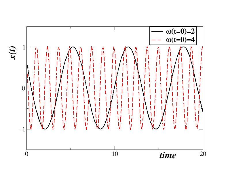
Figure 1: (Color online) Uncoupled oscillators: The time evolution of the $\displaystyle x-$ variable for $\displaystyle\omega(t=0)=2$ (black solid line) and for $\displaystyle\omega(t=0)=4.0$ (red, dashed line). All other parameters are common and are set to: $\displaystyle c=-1$, $\displaystyle\omega_{l}=1$, $\displaystyle\omega_{c}=3$, $\displaystyle\omega_{h}=5$, $\displaystyle R=1$ and $\displaystyle a=1.0$.

III Two-frequency oscillators coupled in a ring network

In this section we couple the two-frequency oscillators in a ring network arrangement. In a network containing $\displaystyle N$ elements, we use the simplest nonlocal coupling scheme where each oscillator is coupled linearly to $\displaystyle 2S$ neighbors: $\displaystyle S$ nearest neighbors on its left and $\displaystyle S$ on its right. Moreover, each $\displaystyle x_{i}-$variable is only coupled to $\displaystyle x_{j}$-variables, $\displaystyle j=i-S,\cdots,i+S$, with common coupling constant $\displaystyle\sigma$. Similarly, each $\displaystyle y_{i}-$variable is only coupled to $\displaystyle y_{j}$-variables, $\displaystyle j=i-S,\cdots,i+S$, with coupling constant $\displaystyle\sigma$, while each $\displaystyle\omega_{i}-$variable is only coupled to $\displaystyle\omega_{j}$-variables, $\displaystyle j=i-S,\cdots,i+S$, with coupling constant $\displaystyle\sigma_{\omega}$. Without loss of generality, we set a common coupling constant, $\displaystyle\sigma$, to the $\displaystyle x_{i}$ and $\displaystyle y_{i}$ variables while a different one, $\displaystyle\sigma_{\omega}$, governs the frequency exchanges. The coupled system of equations takes the form:

$$\displaystyle\frac{dx_{i}}{dt} \displaystyle=-ax_{i}+\frac{aR}{\sqrt{x_{i}^{2}+y_{i}^{2}}}x_{i}-\omega y_{i}+\frac{\sigma}{2S}\sum_{j=i-S}^{i+S}\left[x_{j}-x_{i}\right]$$ (4a)

$$\displaystyle\frac{dy_{i}}{dt} \displaystyle=-ay_{i}+\frac{aR}{\sqrt{x_{i}^{2}+y_{i}^{2}}}y_{i}+\omega x_{i}+\frac{\sigma}{2S}\sum_{j=i-S}^{i+S}\left[y_{j}-y_{i}\right]$$ (4b)

$$\displaystyle\frac{d\omega_{i}}{dt} \displaystyle=c(\omega_{i}-\omega_{l})(\omega_{i}-\omega_{c})(\omega_{i}-\omega_{h})+\frac{\sigma_{\omega}}{2S}\sum_{j=i-S}^{i+S}\left[\omega_{j}-\omega_{i}\right],$$ (4c)

where all indices are taken$\displaystyle\mod{N}$. All oscillators start from random initial conditions in the $\displaystyle(x,y,\omega)$-variables. Assuming that the $\displaystyle\omega_{l}$ and $\displaystyle\omega_{h}$ are the attracting fixed points, the scenario which is now expected to lead to the formation of chimera states has the following logic:

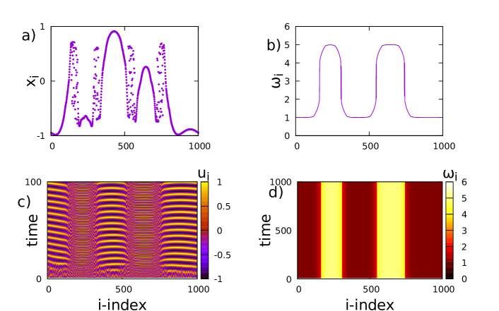
Figure 2: (Color online) The chimera state formed by the two frequency model: a) $\displaystyle x-$variable profile, b) the $\displaystyle\omega$-variable profile c) the space time plot of the $\displaystyle x-$variable and d) the spacetime plot of the $\displaystyle\omega-$variable. Parameters are: $\displaystyle c=-1$, $\displaystyle\omega_{l}=1$, $\displaystyle\omega_{c}=3$, $\displaystyle\omega_{h}=5$, $\displaystyle R=1$, $\displaystyle S=40$, $\displaystyle a=1.0$, $\displaystyle\sigma=0.5$ and $\displaystyle\sigma_{\omega}=3.0$. All simulations start from random initial conditions.

1. As the system integrates, the frequency $\displaystyle\omega_{i}$ of each oscillator will fall on one or the other attracting fixed points $\displaystyle\omega_{l}$ or $\displaystyle\omega_{h}$, depending on their initial $\displaystyle\omega_{i}(t=0)$.

2. Because of the coupling $\displaystyle\sigma_{\omega}$ nearby oscillators will be organized in domains having common frequency, either $\displaystyle\omega_{l}$ or $\displaystyle\omega_{h}$, while the frequencies will alternate in sequential domains.

3. Within each frequency domain the oscillators will have common frequency and due to their coupling, $\displaystyle\sigma$, will also synchronize in phase ($\displaystyle x$- and $\displaystyle y-$variables).

4. Elements in the borders between two frequency domains will be influenced both by their left and right neighbors (have different frequencies $\displaystyle\omega_{l}$ and $\displaystyle\omega_{h}$) and will oscillate asynchronously, creating the asynchronous domains.

5. Such a chimera state arises, with alternating synchronous domains involving two different frequencies (wells), bordered by the asynchronous domains.

As an example, we present in Fig. 2 the chimera state for the working parameter set with specific parameter values: $\displaystyle S=40$, $\displaystyle\sigma=0.5$ and $\displaystyle\sigma_{\omega}=3.0$. In panel a) we present the $\displaystyle x-$variable profile, in panel b) the $\displaystyle\omega$-variable profile and in (c) the spacetime plot of the $\displaystyle x-$variable and in panel d) the space time plot of the $\displaystyle\omega$ profile. A chimera having 4 coherent and 4 incoherent domains is formed. Two of the coherent domains have frequencies $\displaystyle\omega_{l}$ and the other two have $\displaystyle\omega_{h}$, while the incoherent domains form the borders between the coherent ones. This figure will be used as an exemplary case in sec. VI for the comparative spectral analysis of the nodes belonging to the coherent and incoherent regions.

The scenario realized above might be at the basis of the chimera states observed in other systems. It is possible that the combined effects of the nonlinear terms and the coupling in these systems, may induce bistability in their frequencies. If this is the case, then the two-frequency scenarios apply and thus the chimera states are created.

Without loss of generality, in the following sections we use the working parameter set: $\displaystyle c=-1$ (to ensure of the existence of one repulsive fixed point, $\displaystyle\omega_{c}$, surrounded by two attractive ones $\displaystyle\omega_{l}$ and $\displaystyle\omega_{h}$), $\displaystyle\omega_{l}=1$, $\displaystyle\omega_{c}=3$, $\displaystyle\omega_{h}=5$, $\displaystyle R=1$, $\displaystyle S=40$, $\displaystyle a=1.0$, $\displaystyle\sigma=0.5$ and $\displaystyle\sigma_{\omega}=3.0$. Using these parameter values, in section IV we vary the coupling range $\displaystyle S$ and in section V the frequency coupling constant to study the chimera variations under changes of these parameters.

IV Variations with the coupling range

In this section we keep all parameters fixed to the working set and we monitor the chimera properties with variation on the coupling range $\displaystyle S$.

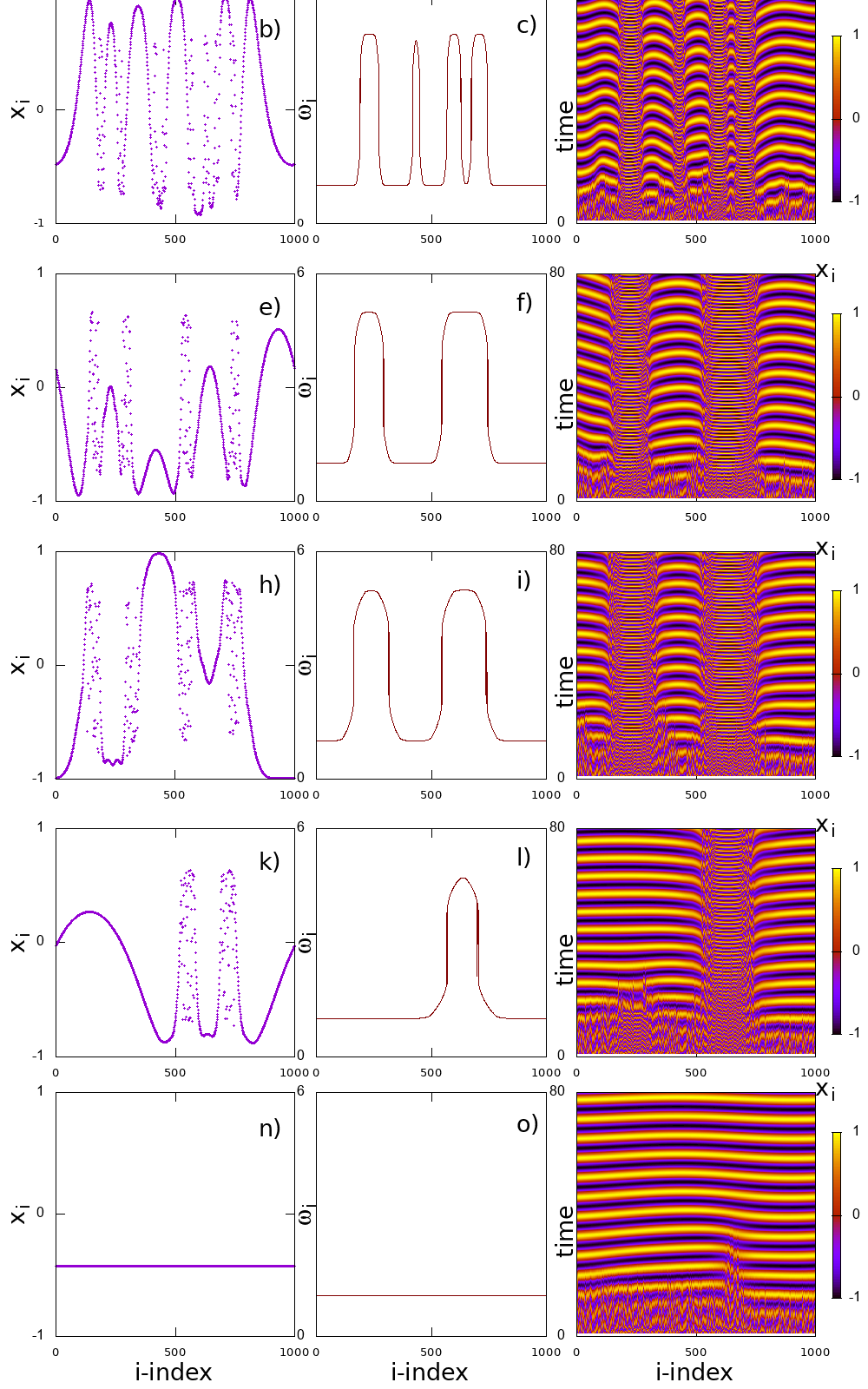
Figure 3: (Color online) Typical chimera state formed by the two frequency model for different values of the coupling range. The plots in the left column depict the $\displaystyle x$-variable profiles, the middle column the mean phase velocities and the right column the spacetime plots of the $\displaystyle x$-variable: a) $\displaystyle S=15$, $\displaystyle x-$variable profile, b) $\displaystyle S=15$, the $\displaystyle\omega$-variable profile c) $\displaystyle S=15$, space time plot of the $\displaystyle x-$variable; d) $\displaystyle S=30$, $\displaystyle x-$variable profile, e) $\displaystyle S=30$, the $\displaystyle\omega$-variable profile f) $\displaystyle S=30$, space time plot of the $\displaystyle x-$variable; g) $\displaystyle S=50$, $\displaystyle x-$variable profile, h) $\displaystyle S=50$, the $\displaystyle\omega$-variable profile i) $\displaystyle S=50$, space time plot of the $\displaystyle x-$variable; j) $\displaystyle S=79$, $\displaystyle x-$variable profile, k) $\displaystyle S=79$, the $\displaystyle\omega$-variable profile l) $\displaystyle S=79$, space time plot of the $\displaystyle x-$variable; m) $\displaystyle S=90$, $\displaystyle x-$variable profile, n) $\displaystyle S=90$, the $\displaystyle\omega$-variable profile o) $\displaystyle S=90$, space time plot of the $\displaystyle x-$variable; Parameters are: $\displaystyle c=-1$, $\displaystyle\omega_{l}=1$, $\displaystyle\omega_{c}=3$, $\displaystyle\omega_{h}=5$, $\displaystyle R=1$, $\displaystyle a=1.0$, $\displaystyle\sigma=0.5$ and $\displaystyle\sigma_{\omega}=3.0$. All runs start from random initial conditions.

In Fig. 3 we depict the evolution of the chimera states for $\displaystyle S=15$ (top line), $\displaystyle S=30$ (second line), $\displaystyle S=50$ (third line), $\displaystyle S=79$ (fourth line), $\displaystyle S=90$ (bottom line). It is clear that small values of the coupling range $\displaystyle S$ give rise to a large number of coherent (and incoherent) regions, while as we increase the size of $\displaystyle S$ the number of coherent (incoherent) regions decrease. For $\displaystyle S>80$ full synchronization is achieved for the working parameter set. This is not unexpected. Provided that the system size remains constant, for large coupling ranges the exchanges between elements cover larger distances, causing communications to larger and larger regions with full synchronization as the ultimate state, see Fig. 3m,n and o.

The decrease in the number of coherent (incoherent) domains with increasing $\displaystyle S$ has also been observed in other systems, such as in FitzHugh-Nagumo Omelchenko et al. (2013), Leaky Integrate-and-Fire Tsigkri-DeSmedt et al. (2017), the Van der Pol Omelchenko et al. (2015) and other oscillator networks Schöll (2016). An intuitive understanding of this effect is that the coupling range defines the region where oscillators interact and thus can synchronize. Therefor, the larger the coupling range, the larger the synchronized regions and consequently fewer synchronous and asynchronous regions can be accommodated by a system of finite, constant length.

In Fig. 4 we present quantitative results on the ratios of elements that belong to the lower frequency domain $\displaystyle\omega_{l}$ (solid, black line), the higher frequency domain $\displaystyle\omega_{h}$ (dashed, red line) and the total number of synchronous elements (dashed-dotted, blue line) as a function of neighborhood size $\displaystyle 2S$. Let us denote by $\displaystyle r=2S/N$, the ratio of coupled elements $\displaystyle 2S$ over the total number of elements $\displaystyle N$ in the network. We may notice three regions where the behavior is distinct: a) Small sizes of coupling ranges $\displaystyle r<0.03$ (or $\displaystyle 2S<30$): Here the number of elements that synchronize close to $\displaystyle\omega_{l}$ ($\displaystyle\omega_{h}$) increases (decreases). b) Intermediate sizes of coupling ranges $\displaystyle 0.04<r<0.15$ (or $\displaystyle 40<2S<150$): Here the number of elements that synchronize close to $\displaystyle\omega_{l}$ decreases and so do the elements that synchronize close to $\displaystyle\omega_{h}$. Around $\displaystyle 2S=160,\>r=0.16$ all elements that have the highest synchronization frequency disappear and the system is left with a synchronous domain at $\displaystyle\omega=\omega_{l}=1$, while the rest of the elements belong to the asynchronous regime. c) Large coupling ranges $\displaystyle r>0.16$ or ($\displaystyle 2S>160$): Here the number of elements that synchronize at $\displaystyle\omega_{l}$ gradually increases and reaches full synchronization beyond $\displaystyle r>0.18,\>2S>180$. This scenario is fairly generic and for large values of the coupling constant one of the two frequency domains dominates at the expense of the other.

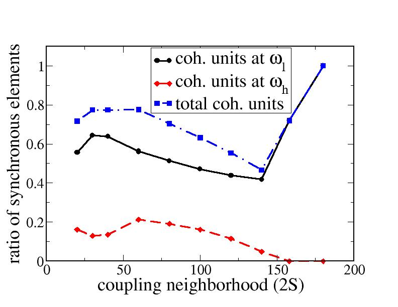
Figure 4: (Color online) Two frequency chimera properties: The ratio of oscillators having frequency $\displaystyle\omega_{l}=1$ (solid, black line), $\displaystyle\omega_{h}=5$ (dashed, red line) and the total number of synchronous elements (dashed-dotted, blue line) as a function of neighborhood size $\displaystyle 2S$. Other parameter values as in Fig. 2.

V Variations with the coupling constants

It is interesting to study the variations of this models with the coupling constants. As in most cases of synchronization in the form of chimera states the coupling constant $\displaystyle\sigma$ which governs the amplitude synchronization does not affect the chimera multiplicity but only the size of coherent and incoherent domains. We shortly discuss this case using an example in the Appendix A. As the exemplary case shows, the size of the incoherent regions decreases as $\displaystyle\sigma$ increases, leading to full synchronization for large values of the coupling strength $\displaystyle\sigma$ .

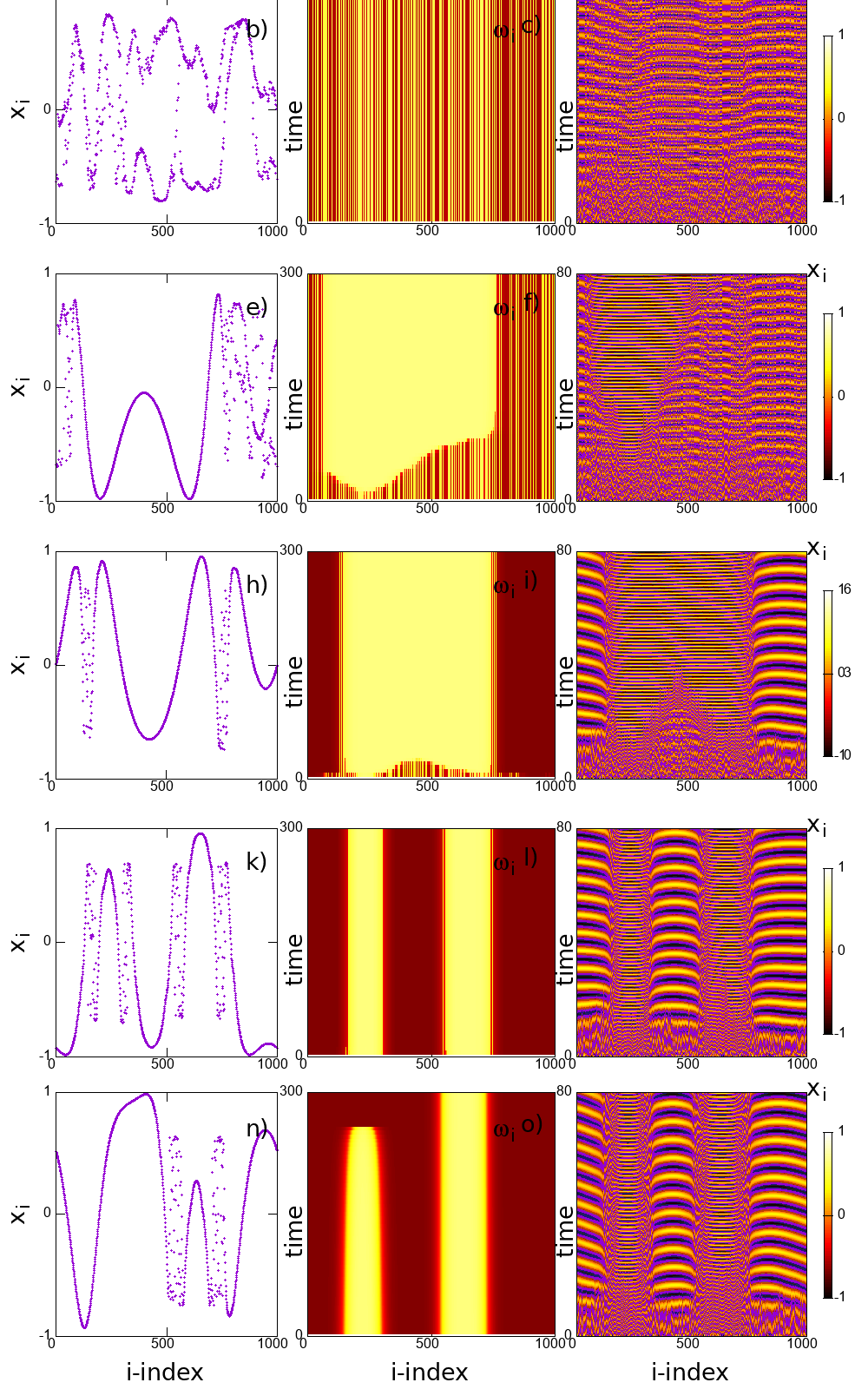
Figure 5: (Color online) Two frequency chimera properties: Left columns are $\displaystyle x$-profiles, middle columns depict $\displaystyle\omega$-and the right columns depict $\displaystyle x$-space time plots. a) $\displaystyle\sigma_{\omega}=1.5$, $\displaystyle x-$variable profile, b) $\displaystyle\sigma_{\omega}=1.5$, spacetime plot of $\displaystyle\omega$-variable c) $\displaystyle\sigma_{\omega}=1.5$, space time plot of $\displaystyle x-$variable; d) $\displaystyle\sigma_{\omega}=1.8$, $\displaystyle x-$variable profile, e) $\displaystyle\sigma_{\omega}=1.8$, spacetime plot of $\displaystyle\omega$-variable, f) $\displaystyle\sigma_{\omega}=1.8$, space time plot of $\displaystyle x-$variable; g) $\displaystyle\sigma_{\omega}=2.0$, $\displaystyle x-$variable profile, h) $\displaystyle\sigma_{\omega}=2.0$, spacetime plot of $\displaystyle\omega$-variable, i) $\displaystyle\sigma_{\omega}=2.0$, space time plot of $\displaystyle x-$variable; j) $\displaystyle\sigma_{\omega}=2.5$, $\displaystyle x-$variable profile, k) $\displaystyle\sigma_{\omega}=2.5$, spacetime plot of $\displaystyle\omega$-variable, l) $\displaystyle\sigma_{\omega}=2.5$, space time plot of $\displaystyle x-$variable; m) $\displaystyle\sigma_{\omega}=5.5$, $\displaystyle x-$variable profile, n) $\displaystyle\sigma_{\omega}=5.5$, spacetime plot of $\displaystyle\omega$-variable, o) $\displaystyle\sigma_{\omega}=5.5$, space time plot of $\displaystyle x-$variable; for $\displaystyle\sigma=$ a) 0.2, b) 0.6, c) 1.0 and d) 1.5. Other parameters are: $\displaystyle c=-1$, $\displaystyle\omega_{l}=1$, $\displaystyle\omega_{c}=3$, $\displaystyle\omega_{h}=5$, $\displaystyle R=1$, $\displaystyle a=1.0$, $\displaystyle S=40$ and $\displaystyle\sigma=0.5$.

After the brief discussion on the amplitude coupling strength, we now turn to the more interesting case of the variations in the frequency coupling range $\displaystyle\sigma_{\omega}$. Figure 5 provides a first account on the formation of the two frequency chimera state as we turn on the coupling on the frequency variables. In the absence or for small values of the $\displaystyle\sigma_{\omega}$ all oscillators fall fast in their attracting fixed points ($\displaystyle\omega_{l}$ or $\displaystyle\omega_{h}$) and they perform oscillations with these frequencies. Neighboring oscillators are not affected and the system remains asynchronous in time. Such an example is presented in the top row of Fig. 5, with $\displaystyle\sigma_{\omega}=1.5$. From the spacetime plot of the mean-phase velocity, Fig. 5b, it is evident that all oscillators acquire a constant in time $\displaystyle\omega_{i}$. As frequency coupling increases in the second row of Fig. 5 to $\displaystyle\sigma_{\omega}=1.5$, a part of the system develops synchronization in the highest frequency, $\displaystyle\omega_{h}=5$, while the rest of the oscillators to the left and right of the synchronous regions have mixed frequencies, see Fig. 5e. This is because the asynchronous regions keep their local frequencies which have been shaped as the oscillators were attracted by fixed points $\displaystyle\omega_{l}$ or $\displaystyle\omega_{h}$. The corresponding $\displaystyle x$-profile, Fig. 5d, demonstrates coherent motion in the synchronous region and incoherent outside of it, while the $\displaystyle x$-spacetime plot, Fig. 5f, indicates that even within the incoherent domain small regions of random sizes are formed with almost coherent temporal behavior. This is not discernible in the $\displaystyle x$-profile but is visible in the spacetime plot.

By increasing further the frequency coupling to $\displaystyle\sigma_{\omega}=2$, see Figs. 5h,i,g, the previously asynchronous domain now synchronizes to the higher frequency, $\displaystyle\omega_{l}$, thus leading to a chimera state consisting of two coherent domains, one in the high frequency, $\displaystyle\omega_{h}=5$ and one in the low frequency $\displaystyle\omega_{l}=1$. Two incoherent domains are develop which serve as the borders between the two coherent ones. The two incoherent domains also serve for continuity purposes to bridge the gap between the domains where $\displaystyle\omega_{h}$ and $\displaystyle\omega_{l}$ dominate. As the frequency coupling increases further to $\displaystyle\sigma_{\omega}=2.5$, see Figs. 5j,k,l, the high frequency domain splits giving rise to four, coherent domains bordered by four incoherent ones. By further increasing $\displaystyle\sigma_{\omega}=5.5$ the exchange of $\displaystyle\omega$ variables become dominant and as time increases the neighboring domains compete and the lower frequency domains expand in expense of the higher ones, see Figs. 5j,k,l. All runs in Fig. 5 start from the same random initial state.

VI Frequency spectra of coherent and incoherent elements

To investigate the transition from the coherent to incoherent regions and to check which precise frequencies are present in each region we investigate the Fourier spectra of different oscillators belonging to the core of the coherent and others occupying borderline regions.

We analyze here the results in Fig. 2 and plot the Fourier spectra of nodes $\displaystyle i=440,\>650$ and $\displaystyle 740$. The first one, $\displaystyle i=440$, is centrally located in the coherent domain which oscillates with $\displaystyle\omega=1$, the second, $\displaystyle i=650$, belongs to the coherent domain with $\displaystyle\omega=5$, while the third one, $\displaystyle i=740$, occupies a position in between the two, in the incoherent region which serves as a transition region between the two domains. The results are shown in Fig. 6.

The left panel of Fig. 6 depicts the Fourier amplitude of node $\displaystyle i=440$. Only one peak is clearly seen at frequency values $\displaystyle f=\omega/2\pi=0.167402$, or $\displaystyle\omega\sim 1$, as expected for the oscillators which have fallen in the basin of attraction of the lowest frequency, $\displaystyle\omega_{l}=1$. The middle panel, Fig. 6b, depicts the Fourier amplitude of node $\displaystyle i=650$. Also here, only one peak is developed at frequency values $\displaystyle f=\omega/2\pi=0.789951$, or $\displaystyle\omega\sim 5$, as expected for the oscillators which have fallen in the basin of attraction of the lowest frequency, $\displaystyle\omega_{h}=5$. The right panel, Fig. 6c, depicts the Fourier amplitude of node $\displaystyle i=740$. Here four peaks appear at frequency values i) $\displaystyle f=\omega/2\pi=0.167402$ ($\displaystyle\omega\sim 1$), ii) $\displaystyle f=\omega/2\pi=0.79$ ($\displaystyle\omega\sim 5$), iii) $\displaystyle f=\omega/2\pi=0.642$ ($\displaystyle\omega\sim 4.03$) and iv) $\displaystyle f=\omega/2\pi=0.496$ ($\displaystyle\omega\sim 3.1$). In these regions the oscillators are developing mixed behavior and present mixed oscillatory characteristics, drawing both from the low frequency dynamics (Case i) and the high frequency dynamics (Case ii). In addition two more peaks with high amplitude are developed which can be considered as linear combinations of the $\displaystyle\omega_{h}$ and $\displaystyle\omega_{l}$ values. E.g., the peak with the highest amplitude in the right panel of Fig. 6 which corresponds to $\displaystyle\omega=4.03$ is approximately equal to $\displaystyle(\omega_{l}+\omega_{h})/2$. Within the incoherent region, the closer the element is to the high (low) frequency domain, the higher the amplitude of the corresponding peak is (images not shown).

These findings corroborate the intuitive argument that the two different types of coherent domains are formed due to the bistability of the oscillator frequency caused by the addition of the linear coupling terms to the nonlinear dynamics. In this view, the incoherent regions serve for the purpose of continuity when passing from the lower to the higher frequency domains (and the opposite). That is the reason why they have a gradient in frequencies, giving rise to the asynchronous incoherent domains in the $\displaystyle x$-variable profile (and $\displaystyle y-$variable profile, not shown).

At this point one would argue that a number of chimera states do not present two-level synchronization, but they demonstrate an arc-shaped mean phase velocity profile. Given the present results, it is not possible to conclude whether the arc-shape $\displaystyle\omega$-profile of the chimera states in the Kuramoto Kuramoto and Battogtokh (2002) or the FitzHugh Nagumo Omelchenko et al. (2013) models emerges as an incompletely formed higher (or lower) frequency domain, or if some other phenomenon is responsible for this profile.

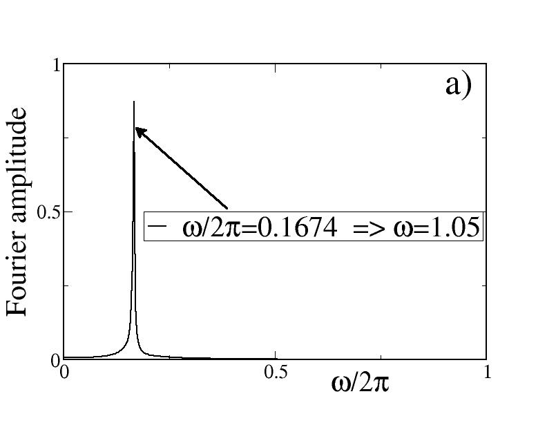
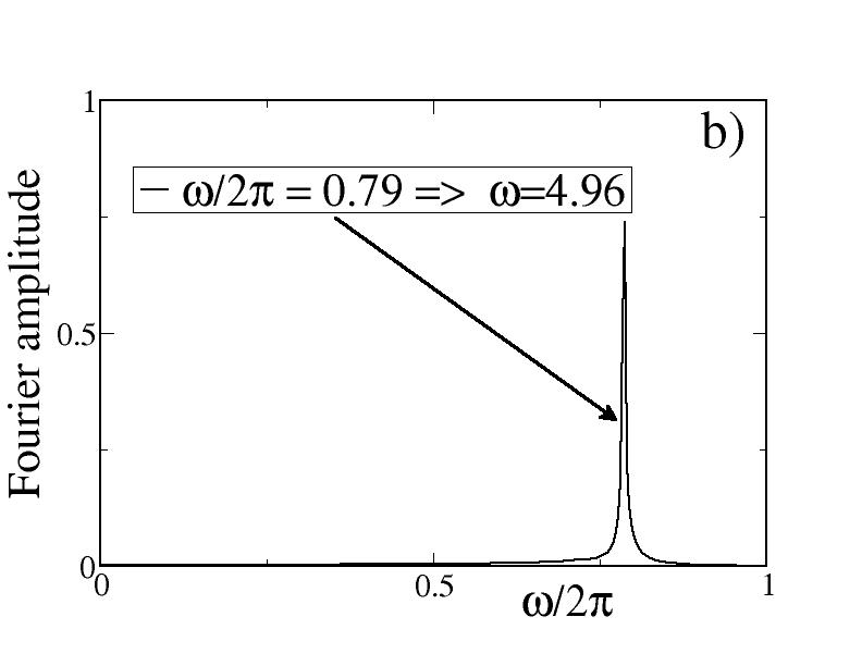
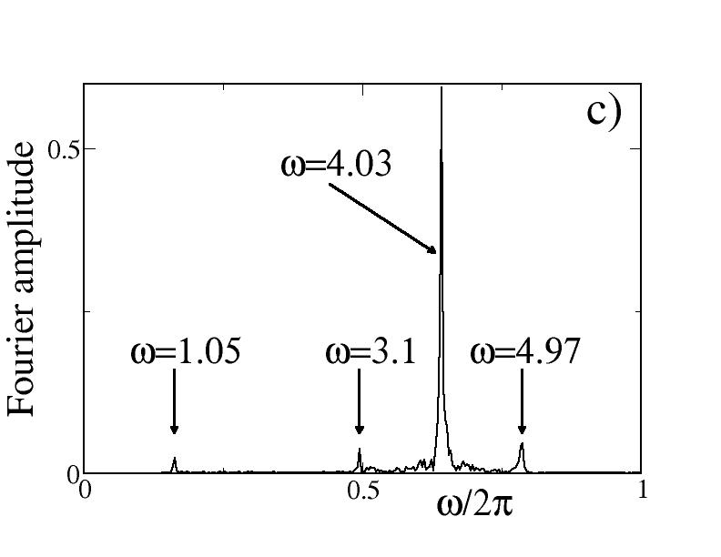
Figure 6: (Color online) Spectral analyses of three nodes referring to the simulation reported in Fig. 2: a) element $\displaystyle i=440$ belonging to the coherent region of low frequency, b) element $\displaystyle i=650$ belonging to the coherent region of high frequency and c) element $\displaystyle i=740$ belonging to incoherent region. All parameter values refer to Fig. 2.

As an additional indicator of the different frequencies dominating in the coherent regions, we plot in Fig. 7 the Fourier amplitude of the peak which corresponds to the low mean phase velocity, $\displaystyle\omega_{l}\sim 1$ (black line) and to the high one, $\displaystyle\omega_{h}\sim 5$ (red line). Comparing Figs. 7 and  2b we note that the Fourier amplitude of the peak at frequencies $\displaystyle\omega\sim 1$ dominates in the coherent regions of low $\displaystyle\omega$ in Fig. 2b and vanishes gradually in domains of high frequency (see Fig. 7, black line). Similarly, the red line which depicts the Fourier amplitude extracted from the the peak at frequencies $\displaystyle\omega\sim 5$ reaches maximum values in the coherent domains of high $\displaystyle\omega$ in Fig. 2b and vanishes in the domains of low frequency. In the intermediate domains, between the low and high frequency ones, the Fourier amplitudes acquire intermediate values. At the same time new peaks appear, as shown in Fig. 6c, whose spectra are the linear combinations of the $\displaystyle\omega_{h}$ and $\displaystyle\omega_{l}$ values. These additional spectral lines, clearly appearing in  6c, are omitted in Fig. 7 for clarity reasons.

The results in this section indicate that the calculation of the Fourier spectra is a laborious but reliable method to identify qualitatively and qualitatively the different coherent and incoherent domains and to assert the presence (or absence) of a chimera state.

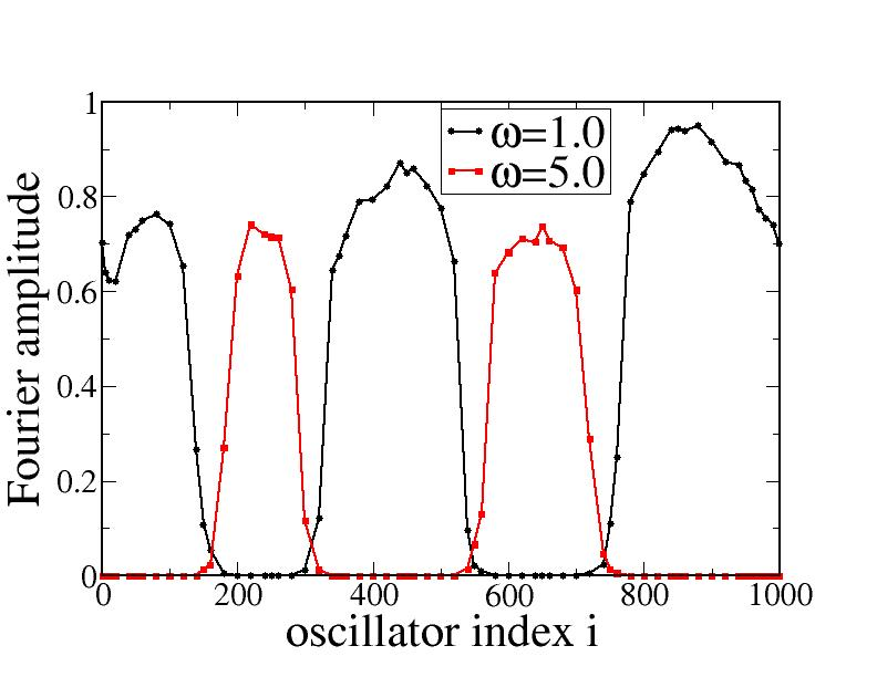
Figure 7: (Color online) Fourier amplitudes of the dynamics of all elements for the numerical results reported in Fig. 2. The black line depicts the Fourier amplitude of the peak which corresponds to the low mean phase velocity, $\displaystyle\omega_{l}\sim 1$ and the red line to the high one, $\displaystyle\omega_{h}\sim 5$. All parameter values refer to Fig. 2.

VII Conclusions

In the present study we first introduced a model oscillator whose trajectory tends exponentially to a closed limiting orbit with well defined frequency and radius. As numerical results indicate, no chimera states arise when such oscillators are coupled, but the system tends to either full synchronization or to full disorder. When a third equation is added which allows the oscillators to choose between two different frequencies, a higher and a lower ones, then domains are formed where the high and low frequencies dominate. The domains of different frequencies are mediated by incoherent domains where the oscillator frequencies gradually increase or decrease to bridge the frequency gap between adjacent regions and to maintain continuity in the system. This scenario can serve as a general mechanism for formation of chimera states. Even in cases where this mechanism is not explicit, the introduction of coupling together with the nonlinearity in the dynamics may induce bistability in the oscillator frequency creating, in this way, indirectly, two-level synchronization and corresponding chimera states.

The present model can be easily extended to form multi-leveled chimeras, by allowing the oscillators to occupy many different frequency levels.

Finally, in Ref. Provata (2018) except for the case of the exponential relaxation to the limiting orbit, power law relaxation has been introduced. Power laws take much longer (infinite time) to reach the final oscillatory trajectory. It would be interesting to investigate whether this power law relaxation dynamics leads also to the formation of chimera states and, further-on, if frequency multistability can lead to multi-leveled chimera states.

Appendix A The role of the amplitude coupling constant

As in most cases of local synchronization in the form of chimera states, the coupling constant $\displaystyle\sigma$ which governs the amplitude synchronization does not affect the chimera multiplicity but only the size of coherent and incoherent domains. As an exemplary case we present here simulation results using the following parameter set: $\displaystyle c=-1$, $\displaystyle\omega_{l}=1$, $\displaystyle\omega_{c}=3$, $\displaystyle\omega_{h}=5$, $\displaystyle R=1$, $\displaystyle a=1.0$, $\displaystyle S=40$ and $\displaystyle\sigma_{\omega}=3.0$, with variable size of $\displaystyle\sigma=0.2,\>0.6,\>1.0$ and $\displaystyle 1.5$. In Fig. A1 the spacetime plots of the variable $\displaystyle x$ are presented in the four cases. For small $\displaystyle\sigma$ values the incoherent regions extend to a large number of oscillator, while the size of the incoherent domains decreases for larger $\displaystyle\sigma$-values.

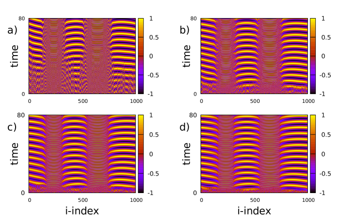
Figure A1: (Color online) Two frequency chimera properties: Spacetime plots for $\displaystyle\sigma=$ a) 0.2, b) 0.6, c) 1.0 and d) 1.5. Other parameters are: $\displaystyle c=-1$, $\displaystyle\omega_{l}=1$, $\displaystyle\omega_{c}=3$, $\displaystyle\omega_{h}=5$, $\displaystyle R=1$, $\displaystyle a=1.0$, $\displaystyle S=40$ and $\displaystyle\sigma_{\omega}=3.0$.

References

- Panaggio and Abrams (2015) M. J. Panaggio and D. Abrams, Nonlinearity 28, R67 (2015).
- Schöll (2016) E. Schöll, European Physical Journal – Special Topics 225, 891 (2016).
- Yao and Zheng (2016) N. Yao and Z. Zheng, International Journal of Modern Physics B 30, 1630002 (2016).
- Omel’Chenko (2018) O. E. Omel’Chenko, Nonlinearity 31, R121 (2018).
- Kuramoto and Battogtokh (2002) Y. Kuramoto and D. Battogtokh, Nonlinear Phenomena in Complex Systems 5, 380 (2002).
- Kuramoto (2002) Y. Kuramoto, in Nonlinear Dynamics and Chaos: Where do we go from here?, edited by S. J. Hogan, A. R. Champneys, A. R. Krauskopf, M. di Bernado, R. E. Wilson, H. M. Osinga, and M. E. Homer (CRC Press, 2002), pp. 209–227.
- Abrams and Strogatz (2004) D. M. Abrams and S. H. Strogatz, Physical Review Letters 93, 174102 (2004).
- Omelchenko et al. (2013) I. Omelchenko, O. E. Omel’chenko, P. Hövel, and E. Schöll, Physical Review Letters 110, 224101 (2013).
- Ulonska et al. (2016) S. Ulonska, I. Omelchenko, A. Zakharova, and E. Schö ll, Chaos 26, 094825 (2016).
- Tumash et al. (2018) L. Tumash, E. Panteley, A. Zakharova, and E. Schöll, European Physical Journal B 92, 100 (2018).
- Gjurchinovski et al. (2017) A. Gjurchinovski, E. Schöll, and A. Zakharova, Physical Review E 95, 042218 (2017).
- Zakharova et al. (2017) A. Zakharova, N. Semenova, V. S. Anishchenko, and E. Schöll, Chaos 27, 114320 (2017).
- Hizanidis et al. (2014) J. Hizanidis, V. Kanas, A. Bezerianos, and T. Bountis, International Journal of Bifurcations and Chaos 24, 1450030 (2014).
- Olmi et al. (2015) S. Olmi, E. A. Martens, S. Thutupalli, and A. Torcini, Physical Review E 92, 030901 (2015).
- Goldschmidt et al. (2019) R. J. Goldschmidt, A. Pikovsky, and A. Politi, Chaos 29, 071101 (2019).
- Tsigkri-DeSmedt et al. (2016) N. D. Tsigkri-DeSmedt, J. Hizanidis, P. Hövel, and A. Provata, European Physical Journal - Special Topics 225, 1149 (2016).
- Shepelev et al. (2017) I. A. Shepelev, A. V. Bukh, G. I. Strelkova, T. E. Vadivasova, and V. S. Anishchenko, Nonlinear Dynamics 90, 2317 (2017).
- Bukh et al. (2017) A. Bukh, E. Rybalova, N. Semenova, G. Strelkova, and V. Anishchenko, Chaos 27, 111102 (2017).
- Malchow et al. (2018) A. K. Malchow, I. Omelchenko, E. Schöll, and P. Hövel, Physical Review E 98, 012217 (2018).
- Martens et al. (2013) E. A. Martens, S. Thutupalli, A. Fourrière, and O. Hallatschek, Proceedings of the National Academy of Sciences 110, 10563 (2013).
- Blaha et al. (2016) K. Blaha, R. J. Burrus, J. L. Orozco-Mora, E. Ruiz-Beltrán, A. B. Siddique, V. D. Hatamipour, and F. Sorrentino, Chaos 26, 116307 (2016).
- Dudkowski et al. (2016) D. Dudkowski, J. Grabski, J. Wojewoda, P. Perlikowski, Y. Maistrenko, and T. Kapitaniak, Scientific Reports 6, 29833 (2016).
- Tinsley et al. (2012) M. R. Tinsley, S. Nkomo, and K. Showalter, Nature Physics 8, 662 (2012).
- Nkomo et al. (2013) S. Nkomo, M. R. Tinsley, and K. Showalter, Physical Review Letters 110, 244102 (2013).
- Taylor et al. (2015) A. F. Taylor, M. R. Tinsley, and K. Showalter, Physical Chemistry Chemical Physics 17, 20047 (2015).
- Rosin et al. (2019) D. P. Rosin, D. Rontani, N. D. Haynes, E. Schöll, and D. J. Gauthier, PHYSICAL REVIEW E 90, 030902(R) (2019).
- English et al. (2017) L. Q. English, A. Zampetaki, P. G. Kevrekidis, K. Skowronski, C. B. Fritz, and S. Abdoulkary, Chaos 27, 103125 (2017).
- M.Hagerstrom et al. (2012) A. M.Hagerstrom, T. E. Murphy, R. Roy, P. Hövel, I. Omelchenko, and E. Schöll, Nature Physics 8, 658 (2012).
- Uy et al. (2019) C. H. Uy, L. Weicker, D. Rontani, and M. Sciamanna, APL Photonics 4, 056104 (2019).
- Rattenborg et al. (2000) N. C. Rattenborg, C. J. Amlaner, and S. L. Lima, Neuroscience and Biobehavioral Reviews 24, 817 (2000).
- Rattenborg (2006) N. C. Rattenborg, Naturwissenschaften 93, 413 (2006).
- Mormann et al. (2000) F. Mormann, K. Lehnertz, P. David, and C. E. Elger, Physica D 144, 358 (2000).
- Mormann et al. (2003) F. Mormann, T. Kreuz, R. G. Andrzejak, P. David, K. Lehnertz, and C. E. Elger, Epilepsy Res. 53, 173 (2003).
- Andrzejak et al. (2016) R. G. Andrzejak, C. Rummel, F. Mormann, and K. Schindler, Scientific Reports 6, 23000 (2016).
- Dudkowski et al. (2014) D. Dudkowski, Y. Maistrenko, and T. Kapitaniak, Physical Review E 90, 032920 (2014).
- Shepelev and Vadivasova (2019) I. Shepelev and T. Vadivasova, Communications in Nonlinear Science and Numerical Simulation 79, 104925 (2019).
- Provata (2018) A. Provata, https://arxiv.org/abs/1803.02080 (2018).
- Tsigkri-DeSmedt et al. (2017) N. D. Tsigkri-DeSmedt, J. Hizanidis, E. Schöll, P. Hövel, and A. Provata, The European Physical Journal B 90, 139 (2017).
- Omelchenko et al. (2015) I. Omelchenko, A. Provata, J. Hizanidis, E. Schöll, and P. Hövel, Physical Review E 91, 022917 (2015).