Solving the quantum master equation of coupled harmonic oscillators with Lie algebra methods

Abstract

Based on a Liouville-space formulation of open systems, we present two methods to solve the quantum dynamics of coupled harmonic oscillators experiencing Markovian loss. Starting point is the quantum master equation in Liouville space which is generated by a Liouvillian that induces a Lie algebra. We show how this Lie algebra allows to define ladder operators that construct Fock-like eigenstates of the Liouvillian. These eigenstates are used to decompose the time-evolved density matrix and, together with the accompanying eigenvalues, provide insight into the transport properties of the lossy system. Additionally, a Wei-Norman expansion of the generated time evolution can be found by a structure analysis of the algebra. This structure analysis yields a construction principle to implement effective non-Hermitian Hamiltonians in lossy systems.

I Introduction

The theory of open quantum systems developed from a bare necessity of describing realistic quantum systems to a tool for their deliberate design. As a result, the non-Hermiticity of open systems was no longer deemed a hindrance but became a potential resource of interesting effects in its own right. In recent years, interest in such non-Hermitian systems soared spanning from investigations of parity-time ($\mathcal{PT}$) symmetry BenderBoettcher , which preserves the reality of the spectrum of the Hamiltonian, over non-Hermitian coalescence of modes at exceptional points (EP) Heiss , to fundamental questions regarding generalisations to non-Hermitian quantum mechanics Brody .

Experimental realisations of $\mathcal{PT}$ symmetry or exceptional points can be found especially in optical systems Miri2019 ; Rueter ; Peng due to their high level of control over the gain and loss, but other implementations exist such as LC circuits Schindler , microwave cavities Dembowski , or atoms Zhang . Usually, these implementations are based on classical wave mechanics that account for first-quantisation effects where loss and gain are modelled by an effective non-Hermitian Hamiltonian. For the early research this was sufficient and resulted in many interesting discoveries such as changes of transport behaviour in broken and unbroken $\mathcal{PT}$ symmetry Makris or increased measurement sensitivity at EPs Hodaei .

However, recently efforts have been made to also investigate second-quantisation effects in non-Hermitian systems with one successful example being the measurement of two-photon Hong-Ou-Mandel correlations in a $\mathcal{PT}$-symmetric waveguide coupler Klauck19 . The key step was the use of passive $\mathcal{PT}$ symmetry meaning that the required antisymmetric gain/loss distribution was replaced by an all-loss distribution with the same antisymmetry. This passive scheme was used because any gain added to the system also adds noise that irrevocably changes the quantum state under study which negatively affects the observance of any $\mathcal{PT}$ quantum effect Scheel . Thus, the replacement of gain/loss structures by pure loss structures seems to be one way to implement non-Hermitian quantum dynamics.

In this work, we present a theoretical description of the quantum dynamics of lossy quantum systems that lays the foundations to further understand the quantum effects occurring in non-Hermitian systems which might pave the way to investigate and apply quantum $\mathcal{PT}$ symmetry and quantum EPs. For this, we present two methods to obtain the dynamics of coupled quantum harmonic oscillators experiencing Markovian losses. Such oscillator systems model lossy waveguide arrays but are also applicable to other systems of bosonic nature. Starting point of our investigation is the quantum master equation in Lindblad form in Liouville space Ban93 . The concept of Liouville space to describe the evolution of the density matrix is well known and allows for a treatment similar to the Schrödinger equation in Hermitian quantum physics, with the difference that the Hamiltonian is replaced by a Liouvillian as the generator of the quantum master equation. The resulting time evolution is found by studying the induced Lie algebraic structure of this Liouvillian, either by diagonalisation of its regular representation, or by a Wei-Norman expansion.

The article is organised as follows. We begin our investigation with a discussion of the Liouville-space formalism in Sec. II where we introduce the system under study and formulate its generating Liouvillian. In Sec. III we discuss how Lie algebraic structures emerge from this Liouvillian and prepare the ground to establish the methods for solving the quantum dynamics. Section IV focusses on solving the quantum dynamics for fixed system parameters by means of an eigendecomposition of the Liouvillian. The second method is a Wei-Norman expansion which is the subject of Sec. V which leads to deeper insight into the underlying algebraic structure. Concluding remarks can be found in Sec. VI. Some details regarding Liouville-space ladder operators and structure analysis in the Wei-Norman expansion have been relegated to the Appendix.

II Liouville space formalism

We begin our investigation by introducing the Liouville-space formalism Ban93 and show how to apply it to a system of coupled harmonic oscillators experiencing Markovian loss. A Liouville space $\mathfrak{L}$ is the Cartesian product of two Hilbert spaces. When used to describe open quantum systems, the involved spaces are usually the Hilbert space $\mathcal{H}$ of a closed system and its dual $\mathcal{H}^{\prime}$, i.e. $\mathfrak{L}=\mathcal{H}\otimes\mathcal{H}^{\prime}$. This effectively elevates the description from the quantum states $|\psi\rangle\in\mathcal{H}$ to the density matrices $\hat{\rho}\in\mathfrak{L}$. Operators in the Hilbert space $\hat{A}\in\mathcal{H}$ then become vectors in $\mathfrak{L}$ and are represented by double kets $|A\rangle\rangle$. For these vectors, one can define a new inner product $\langle\langle A|B\rangle\rangle=\mathrm{Tr}\left(\hat{A}^{\dagger}\hat{B}\right)$. In conjunction with this inner product, the Liouville space is itself a Hilbert space allowing many properties to be carried over to $\mathfrak{L}$, in particular notions such as projections and completeness. However, for this to be true some detailed attention has to be paid to the dual elements $\langle\langle A|$. The reason is that, in general, the dual space does not equal the Liouville space itself which is especially true for non-Hermitian open systems. This problem can be treated rigorously in the framework of rigged Hilbert spaces Gelfand , and it can be shown Honda that the Liouville space constructed from the Hilbert space spanned by bosonic Fock states does possess a complete basis.

When transitioning from the original Hilbert space to its derived Liouville space, the quantum dynamics is no longer given by the Schrödinger equation but by the von-Neumann equation, i.e.

$$\mathrm{i}\frac{\mathrm{d}}{\mathrm{d}t}|\psi\rangle=\hat{H}|\psi\rangle\qquad\rightarrow\qquad\frac{\mathrm{d}}{\mathrm{d}t}|\rho\rangle\rangle=\mathcal{L}|\rho\rangle\rangle.$$ (1)

Here we introduced the Liouvillian $\mathcal{L}$ as a superoperator acting solely to the right. In order to define such a right action, superoperators can often be defined as left or right applications of Hilbert-space operators. For example, one can derive the two Liouville space superoperators $L[\hat{O}]$ and $R[\hat{O}]$ from the Hilbert space operator $\hat{O}$ as

$$L[\hat{O}]|A\rangle\rangle=\hat{O}\hat{A},$$

$$R[\hat{O}]|A\rangle\rangle=\hat{A}\hat{O}.$$

This principle shall now be applied to a linear chain of $N$ coupled harmonic oscillators. The closed system Hamiltonian is

$$\hat{H}=\sum_{k=1}^{N}\sigma_{k}\hat{a}_{k}^{\dagger}\hat{a}_{k}+\sum_{k=1}^{N-1}\kappa_{k}\left(\hat{a}_{k}^{\dagger}\hat{a}_{k+1}+\hat{a}_{k}\hat{a}_{k+1}^{\dagger}\right)$$ (2)

with the bosonic mode operators $\hat{a}_{k}$, $\hat{a}_{k}^{\dagger}$, the energy $\sigma_{k}$ of the $k$th mode, and the coupling $\kappa_{k}$ between modes $k$ and $k+1$. Such a Hamiltonian is often encountered, for example, when modelling light propagation in photonic waveguides Meany ; Linares .

Loss in the $k$th mode is introduced to the system as Markovian loss of a single excitation with rate $\gamma_{k}$ which, e.g., in photonic waveguides is due to scattering Guo81 . This is modelled by Lindblad terms in the von Neumann equation which then becomes the quantum master equation

$$\frac{\mathrm{d}}{\mathrm{d}t}\hat{\rho}=-\mathrm{i}\left[\hat{H},\hat{\rho}\right]+\sum_{k=1}^{N}\gamma_{k}\left(2\,\hat{a}_{k}\hat{\rho}\hat{a}_{k}^{\dagger}-\left\{\hat{a}_{k}^{\dagger}\hat{a}_{k},\hat{\rho}\right\}\right),$$ (3)

where we used $\{\bullet,\bullet\}$ to denote the anticommutator.

An interesting reformulation of the quantum master equation can be found by grouping the anticommutator term containing the Lindblad operators together with the commutator containing the Hamiltonian of the closed system by defining an effective non-Hermitian Hamiltonian $\hat{H}_{\text{eff}}$,

$$-\mathrm{i}\left[\hat{H},\hat{\rho}\right]-\sum_{k=1}^{N}\gamma_{k}\left\{\hat{a}_{k}^{\dagger}\hat{a}_{k},\hat{\rho}\right\}=-\mathrm{i}\left(\hat{H}_{\text{eff}}\hat{\rho}-\hat{\rho}\hat{H}^{\dagger}_{\text{eff}}\right),$$ (4)

where we added the loss rate to the propagation constant, i.e. $\sigma_{k}\rightarrow\sigma_{k}-\mathrm{i}\gamma_{k}$. Such a term would occur if one would derive the von Neumann equation directly from the Schrödinger equation generated by the non-Hermitian $\hat{H}_{\text{eff}}$. However, without the trace-preserving terms $2\,\gamma_{k}\hat{a}_{k}\hat{\rho}\hat{a}_{k}^{\dagger}$ this effective Hamiltonian does not generate a physical evolution for the whole quantum state by itself. Nonetheless, in Sec. V we will see that it still plays an important role.

Using the bosonic mode operators we can now define a suitable set of superoperators

$$L_{k}^{-}|A\rangle\rangle=\hat{a}_{k}\hat{A},\qquad L_{k}^{+}|A\rangle\rangle=\hat{a}_{k}^{\dagger}\hat{A},$$ (5)

$$R_{k}^{-}|A\rangle\rangle=\hat{A}\hat{a}_{k}^{\dagger},\qquad R_{k}^{+}|A\rangle\rangle=\hat{A}\hat{a}_{k}.$$ (6)

With these, the Liouvillian can solely be defined as a right-action superoperator

$$\mathcal{L}=\sum\limits_{k=1}^{N}\Big{[}\left(\mathrm{i}\sigma_{k}-\gamma_{k}\right)R_{k}^{+}R_{k}^{-}-\left(\mathrm{i}\sigma_{k}+\gamma_{k}\right)L_{k}^{+}L_{k}^{-}$$

$$+2\gamma_{k}L_{k}^{-}R_{k}^{-}\Big{]}$$

$$-\sum\limits_{k=1}^{N-1}\mathrm{i}\kappa_{k}\left(L_{k}^{+}L_{k+1}^{-}+L_{k+1}^{+}L_{k}^{-}-R_{k+1}^{+}R_{k}^{-}-R_{k}^{+}R_{k+1}^{-}\right).$$ (7)

Now that an explicit formulation of a right action is known we can also define a time-evolution superoperator $\mathcal{U}$ in Liouville space that yields the formal solution $|\rho(t)\rangle\rangle=\mathcal{U}(t)|\rho_{0}\rangle\rangle$. This time-evolution superoperator $\mathcal{U}$ obeys the differential equation

$$\frac{\mathrm{d}}{\mathrm{d}t}\mathcal{U}(t)=\mathcal{L}\,\mathcal{U}(t),\qquad\mathcal{U}(0)=\bm{1}_{\mathcal{L}}.$$ (8)

In the following, we will discuss two approaches to solve the quantum master equation (3) based on Lie algebras induced by Eq. (7). The first approach is to find an eigendecomposition of a constant Liouvillian $\mathcal{L}\neq\mathcal{L}(t)$ that allows us to find an explicit form of the formal solution $\mathcal{U}=\mathrm{e}^{t\mathcal{L}}$. The second approach is applicable to a time-dependent Liouvillian $\mathcal{L}(t)$ and is based on a Wei-Norman expansion of $\mathcal{U}$. Both approaches are based on different Lie algebras induced by $\mathcal{L}$. Thus, we first discuss how to generate those algebras from the explicit representation as seen in Eq. (7).

III Induced Lie algebras

From the considerations in the last section we can deduce that the linear chain of $N$ lossy harmonic oscillators are described by $2N$ Hilbert-space operators $\{\hat{a}_{i},\hat{a}_{i}^{\dagger}\}$ that result in $4N$ Liouville-space operators $\{L_{i}^{\pm},R_{i}^{\pm}\}$. Those superoperators inherit their commutation relations from the canonical commutator $[\hat{a}_{i},\hat{a}_{j}^{\dagger}]=\delta_{ij}$ of the Hilbert-space ladder operators. Explicitly, we find

$$[L_{i}^{-},L_{j}^{+}]=\delta_{ij},\quad[R_{i}^{-},R_{j}^{+}]=\delta_{ij}.$$ (9)

Based on these fundamental commutators one can construct a Lie algebra spanned by all linear operators $\{L_{i}^{\pm},R_{i}^{\pm}\}$, all bilinear or quadratic operators $\{L_{i}^{+}L_{j}^{-},R_{i}^{+}R_{j}^{-},L_{i}^{-}R_{j}^{-}\}$, and the Liouville-space identity $\bm{1}_{\mathfrak{L}}$. Note that we included all mode combinations $i,j$ which derives from the fact that commutators such as $[L_{i}^{+}L_{i+1}^{-},L_{i+1}^{+}L_{i+2}^{-}]=L_{i}^{+}L_{i+2}^{-}$ occur. Hence, for the algebra to be closed we have to consider not only the nearest-neighbour coupling operators such as $L_{i}^{+}L_{i+1}^{-}$ that already occur in $\mathcal{L}$, but all other combinations as well. For this reason, the chosen linear-chain arrangement of the oscillators is only for ease of calculations and does not hinder the application to more complicated mode-coupling schemes. Also note that one only needs to include the loss operators $L_{i}^{-}R_{j}^{-}$ as gain does not occur.

A closer inspection of the structure constants of the algebra spanned by $\{\bm{1}_{\mathfrak{L}},L_{i}^{\pm},R_{i}^{\pm},L_{i}^{+}L_{j}^{-},R_{i}^{+}R_{j}^{-},L_{i}^{-}R_{j}^{-}\}$ reveals that the linear operators, together with the identity, constitute an ideal of the whole algebra. Thus, they can be separated to form their own subalgebra. When including the Liouvillian $\mathcal{L}$ to this subalgebra we obtain a closed algebra spanned by $\{\bm{1}_{\mathfrak{L}},L_{i}^{\pm},R_{i}^{\pm},\mathcal{L}\}$ that can be used to find an eigendecomposition of $\mathcal{L}$. Likewise, as $\mathcal{L}$ can be represented solely by the quadratic operators, see Eq. (7), we can construct a closed subalgebra from them that leads to a Wei-Norman expansion of $\mathcal{L}$. Both closed algebras provide us with deeper insight into the lossy oscillator system and yield methods to solve the quantum master equation.

IV Eigendecomposition of the Liouvillian

The first method solves the quantum master equation for a time-independent Liouvillian $\mathcal{L}$ by means of a diagonalisation of its regular representation $\mathcal{R}(\mathcal{L})$. The regular representation of an element $Z$ of a Lie algebra spanned by $\{X_{i}\}$ is defined as

$$\mathcal{R}(Z):[Z,X_{i}]=\mathcal{R}_{ij}(Z)X_{j}$$ (10)

and is thus intricately linked to its inherent structure constants. In case of the algebra spanned by $\{\bm{1}_{\mathfrak{L}},L_{i}^{\pm},R_{i}^{\pm},\mathcal{L}\}$, $\mathcal{R}(Z)$ is a $(4N+2)\times(4N+2)$-matrix. However, as we are only interested in $\mathcal{R}(\mathcal{L})$, we can drop the identity and $\mathcal{L}$ itself and focus on the smaller matrix $\mathcal{R}^{\prime}(\mathcal{L})$ with elements $X_{i}$ drawn only from the linear operators $\{L_{i}^{\pm},R_{i}^{\pm}\}$. When arranging those linear operators as $\{L_{1}^{+},\dots,L_{N}^{+},R_{1}^{-},\dots,R_{N}^{-},R_{1}^{+},\dots,R_{N}^{+},L_{1}^{-},\dots,L_{N}^{-}\}$, the regular representation becomes

$$\mathcal{R}^{\prime}(\mathcal{L})=\begin{pmatrix}-\mathrm{i}\bm{H}_{\text{eff}}&\bm{\Gamma}&\bm{0}&\bm{0}\\ \bm{0}&-\mathrm{i}\bm{H}^{\dagger}_{\text{eff}}&\bm{0}&\bm{0}\\ \bm{0}&\bm{0}&\mathrm{i}\bm{H}^{\dagger}_{\text{eff}}&\bm{\Gamma}\\ \bm{0}&\bm{0}&\bm{0}&\mathrm{i}\bm{H}_{\text{eff}}\end{pmatrix}$$ (11)

with $\bm{\Gamma}=2\,\mathrm{diag}(\gamma_{1},\dots,\gamma_{N})$ and

$$\bm{H}_{\text{eff}}=\begin{pmatrix}\sigma_{1}-\mathrm{i}\gamma_{1}&\kappa_{1}&&\\ \kappa_{1}&\ddots&\ddots&\\ &\ddots&\ddots&\kappa_{N-1}\\ &&\kappa_{N-1}&\sigma_{N}-\mathrm{i}\gamma_{N}\end{pmatrix}.$$ (12)

Diagonalisation of $\mathcal{R}^{\prime}(\mathcal{L})$ yields $4N$ eigenvalues

$$\{\lambda_{1},\dots,\lambda_{N},-\lambda_{1}^{*},\dots,-\lambda_{N}^{*},\lambda_{1}^{*},\dots,\lambda_{N}^{*},-\lambda_{1},\dots,-\lambda_{N}\},$$ (13)

where $\lambda_{i}$ are the eigenvalues of $-\mathrm{i}\bm{H}_{\text{eff}}$. Their accompanying eigenvectors define $4N$ superoperators that are superpositions of the linear operators $L_{i}^{\pm},R_{i}^{\pm}$, and which we split into two equally large groups denoted by $P_{i}^{\pm}$ and $Q_{i}^{\pm}$. They have the general form

$$P^{+}_{i}=\sum_{k}c_{ik}(L^{+}_{k}-R^{-}_{k}),\quad P^{-}_{i}=\sum_{k}c_{ik}L^{-}_{k},$$ (14)

$$Q^{+}_{i}=\sum_{k}c^{*}_{ik}(R^{+}_{k}-L^{-}_{k}),\quad Q^{-}_{i}=\sum_{k}c^{*}_{ik}R^{-}_{k}.$$ (15)

These new superoperators act as collective creation and annihiliation operators in Liouville space. In fact, after suitable normalisation, they obey the commutator relations

$$[P_{i}^{-},P_{j}^{+}]=\delta_{ij},\quad[Q_{i}^{-},Q_{j}^{+}]=\delta_{ij},$$ (16)

with all other commutators vanishing. Furthermore, because they diagonalise the regular representation $\mathcal{R}^{\prime}(\mathcal{L})$, they yield the eigenvalue commutator relations

$$\left[\mathcal{L},P_{i}^{+}\right]=\lambda_{i}P_{i}^{+},\quad\left[\mathcal{L},P_{i}^{-}\right]=-\lambda_{i}P_{i}^{-},$$

$$\left[\mathcal{L},Q_{i}^{+}\right]=\lambda_{i}^{*}Q_{i}^{+},\quad\left[\mathcal{L},Q_{i}^{-}\right]=-\lambda_{i}^{*}Q_{i}^{-}.$$ (17)

These commutators are reminiscent of the ladder operators in Hilbert space which is the reason why we termed them creation and annihiliation operators that add/subtract collective excitations of $\pm\lambda_{i}$ or $\pm\lambda_{i}^{*}$ in Liouville space. Note, however, that these are not physical excitations but are only to be understood as abstract excitations in $\mathfrak{L}$ because they contain creation and annihiliation operators from the original Hilbert space $\mathcal{H}$.

Nonetheless, the Liouville space ladder operators can be used to construct eigenvectors of the Liouvillian $\mathcal{L}$. First, we define a ground state $|0\rangle\rangle$ via

$$P_{i}^{-}|0\rangle\rangle=Q_{i}^{-}|0\rangle\rangle=0,\qquad\forall i,$$ (18)

$$\langle\langle 0|P_{i}^{+}=\langle\langle 0|Q_{i}^{+}=0,\qquad\forall i,$$ (19)

where one has to keep in mind that, due to the non-Hermiticity of $\mathcal{L}$, the left and right vectors are different. A careful analysis leads to

$$|0\rangle\rangle=|\bm{0}\rangle\langle\bm{0}|,\quad\langle\langle 0|=\bm{1}_{\mathcal{H}}$$ (20)

with $\bm{1}_{\mathcal{H}}$ as the identity in the base Hilbert space, see Appendix A. Higher rungs of the ladder are then obtained as

$$|\bm{\alpha},\bm{\beta}\rangle\rangle =\frac{1}{\sqrt{\bm{\alpha}!\bm{\beta}!}}\bm{P}^{+\,\bm{\alpha}}\bm{Q}^{+\,\bm{\beta}}|0\rangle\rangle$$ (21)

$$\langle\langle\bm{\alpha},\bm{\beta}| =\frac{1}{\sqrt{\bm{\alpha}!\bm{\beta}!}}\langle\langle 0|\bm{P}^{-\,\bm{\alpha}}\bm{Q}^{-\,\bm{\beta}},$$ (22)

with multiindeces $\bm{\alpha}=(\alpha_{1},\dots,\alpha_{N})$.

The Liouville-space ladder states are eigenstates of the Liouvillian $\mathcal{L}$ which can be seen by using the commutators (17) and the fact that $\mathcal{L}|0\rangle\rangle=0$. Similarly, we can calculate the action of the evolution operator $\mathcal{U}=\mathrm{e}^{t\mathcal{L}}$ on the states $|\bm{\alpha},\bm{\beta}\rangle\rangle$ via the adjoint action defined by

$$\mathrm{e}^{A}B\mathrm{e}^{-A}=B+[A,B]+\frac{1}{2}[A,[A,B]]+\dots$$ (23)

Applying this to the product of creation operators yields after straightforward calculation

$$\mathrm{e}^{t\mathcal{L}}\bm{P}^{+\,\bm{\alpha}}\bm{Q}^{+\,\bm{\beta}}=\mathrm{e}^{t\mathcal{L}}\bm{P}^{+\,\bm{\alpha}}\bm{Q}^{+\,\bm{\beta}}\mathrm{e}^{-t\mathcal{L}}\mathrm{e}^{t\mathcal{L}}$$

$$=\mathrm{e}^{t\,(\bm{\alpha}\cdot\bm{\lambda}+\bm{\beta}\cdot\bm{\lambda}^{*})}\bm{P}^{+\,\bm{\alpha}}\bm{Q}^{+\,\bm{\beta}}\mathrm{e}^{t\mathcal{L}},$$ (24)

with $\bm{\lambda}=(\lambda_{1},\dots,\lambda_{N})$. The action on a ladder state thus becomes

$$\mathrm{e}^{t\mathcal{L}}|\bm{\alpha},\bm{\beta}\rangle\rangle=\mathrm{e}^{t\,(\bm{\alpha}\cdot\bm{\lambda}+\bm{\beta}\cdot\bm{\lambda}^{*})}|\bm{\alpha},\bm{\beta}\rangle\rangle.$$ (25)

With this result, the time-evolved quantum state is

$$|\rho(t)\rangle\rangle=\mathrm{e}^{t\mathcal{L}}|\rho_{0}\rangle\rangle=\sum_{\bm{\alpha},\bm{\beta}}\mathrm{e}^{t\,(\bm{\alpha}\cdot\bm{\lambda}+\bm{\beta}\cdot\bm{\lambda}^{*})}|\bm{\alpha},\bm{\beta}\rangle\rangle\langle\langle\bm{\alpha},\bm{\beta}|\rho_{0}\rangle\rangle.$$ (26)

The sum runs over all possible multiindices which, however, in practice are limited to a select few. In fact, for an initial state $\hat{\rho}_{0}$ containing $N_{\text{p}}$ bosonic excitations, the multiindices are restricted by $|\bm{\alpha}|,|\bm{\beta}|\leq N_{\text{p}}$.

The expression Eq. (26) is an analytic solution to the quantum master equation (3) of a fixed system of coupled lossy harmonic oscillators. For a few modes and excitations, explicit results can be calculated by hand. For example, let us consider the case of two harmonic oscillators ($N=2$). We define the differences of the propagation constants $\sigma_{1}$ and $\sigma_{2}$ and loss rates $\gamma_{1}$ and $\gamma_{2}$ as well as their respective means as

$$\Delta\sigma=\frac{\sigma_{1}-\sigma_{2}}{2},\qquad\overline{\sigma}=\frac{\sigma_{1}+\sigma_{2}}{2},$$ (27)

$$\Delta\gamma=\frac{\gamma_{1}-\gamma_{2}}{2},\qquad\overline{\gamma}=\frac{\gamma_{1}+\gamma_{2}}{2}.$$ (28)

Together with the (single) coupling rate $\kappa_{1}=\kappa$ we find for the two eigenvalues of $-\mathrm{i}\bm{H}_{\text{eff}}$

$$\lambda_{1}=-\overline{\gamma}-\mathrm{i}\overline{\sigma}+\mathrm{i}\omega,\quad\lambda_{2}=-\overline{\gamma}-\mathrm{i}\overline{\sigma}-\mathrm{i}\omega,$$ (29)

with

$$\omega=\sqrt{\kappa^{2}+(\Delta\sigma-\mathrm{i}\Delta\gamma)^{2}}.$$ (30)

From these, the eight eigenvalues of the Liouvillian are constructed as in Eq. (13). The diagonalisation of the regular representation $\mathcal{R}^{\prime}(\mathcal{L})$ yields two sets of bosonic ladder superoperators, the first being

$$P_{i}^{+}=\epsilon_{i}\left(L_{1}^{+}-R_{1}^{-}\right)+\tau_{i}\left(L_{2}^{+}-R_{2}^{-}\right),$$ (31)

$$P_{i}^{-}=\epsilon_{i}L_{1}^{-}+\tau_{i}L_{2}^{-}$$ (32)

and the second

$$Q_{i}^{+}=\epsilon_{i}^{*}\left(R_{1}^{+}-L_{1}^{-}\right)+\tau_{i}^{*}\left(R_{2}^{+}-L_{2}^{-}\right),$$ (33)

$$Q_{i}^{-}=\epsilon_{i}^{*}R_{1}^{-}+\tau_{i}^{*}R_{2}^{-}$$ (34)

with

$$\epsilon_{1}=\frac{-\kappa}{\sqrt{2\omega(\omega+\Delta\sigma-\mathrm{i}\Delta\gamma)}},\;\;\tau_{1}=\frac{\omega+\Delta\sigma-\mathrm{i}\Delta\gamma}{\sqrt{2\omega(\omega+\Delta\sigma-\mathrm{i}\Delta\gamma)}},$$ (35)

$$\epsilon_{2}=\frac{\kappa}{\sqrt{2\omega(\omega-\Delta\sigma+\mathrm{i}\Delta\gamma)}},\;\;\tau_{2}=\frac{\omega-\Delta\sigma+\mathrm{i}\Delta\gamma}{\sqrt{2\omega(\omega-\Delta\sigma+\mathrm{i}\Delta\gamma)}}.$$ (36)

With the ladder superoperators at hand, the overlap $\langle\langle\bm{\alpha},\bm{\beta}|\rho_{0}\rangle\rangle$ from Eq. (26) can be straightforwardly calculated using the definition of the Liouville space inner product and the construction rule for the left eigenvectors of $\mathcal{L}$ in Eq. (22) as

$$\langle\langle\bm{\alpha},\bm{\beta}|\rho_{0}\rangle\rangle=\frac{\mathrm{Tr}\left(P_{1}^{-\,\alpha_{1}}P_{2}^{-\,\alpha_{2}}Q_{1}^{-\,\beta_{1}}Q_{2}^{-\,\beta_{2}}\hat{\rho}_{0}\right)}{\sqrt{\alpha_{1}!\beta_{1}!\alpha_{2}!\beta_{2}!}}.$$ (37)

This expression depends on the input state $\hat{\rho}_{0}$ and determines which eigenvectors $|\bm{\alpha},\bm{\beta}\rangle\rangle$ have to be considered. Together with the exponential function involving the eigenvalues $\lambda_{i}$ and $\lambda_{i}^{*}$ one can then calculate the time-evolved state and thus any observable.

This method is well suited to theoretically describe the experiment on passive $\mathcal{PT}$-symmetric waveguide couplers Klauck19 . The coupler consisted of two waveguides at a fixed spatial separation, and hence with a fixed coupling strength, where in one of them a loss rate $\gamma$ was introduced by periodic bending of the waveguide. In the experiments, the effect of the loss, and with that of the increasing non-Hermiticity, on the coincidence rate $\Gamma=\langle\hat{a}_{1}^{\dagger}\hat{a}_{2}^{\dagger}\hat{a}_{1}\hat{a}_{2}\rangle$ for detecting two photons was measured. The two photons were initially launched in each waveguide separately, i.e. the initial state was $|1,1\rangle$. The analytical solution for $\Gamma$ can be easily calculated using the above method and reads

$$\Gamma=\mathrm{e}^{-2\gamma t}\left|\frac{\gamma^{2}-4\kappa^{2}\cos\left(t\sqrt{4\kappa^{2}-\gamma^{2}}\right)}{4\kappa^{2}-\gamma^{2}}\right|^{2}.$$ (38)

In Fig. 1, the coincidence rate for two values of the loss $\gamma$ is plotted against the normalised time $\kappa t$. In the Hermitian case $\gamma=0$ (blue line) the well-known result from the Hong-Ou-Mandel experiment is reproduced. The photons bunch at $\kappa t=\pi/4$ and leave the system together in either of the two modes. With increased non-Hermiticity, however, the bunching (red vertical line) is shifted to shorter values of $\kappa t$ with one example with $\gamma=\kappa$ shown (orange dashed). Note that the $\mathcal{PT}$ phase is limited to $\gamma\leq 2\kappa$, the grey area shows the maximal extend of the shift down to $\kappa t=1/\sqrt{2}$. In Ref. Klauck19 , these prediction where experimentally confirmed.

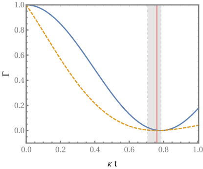
Figure 1: The coincidence function (38) of two coupled harmonic oscillators, one of which experiences loss $\gamma$, with an initial excitation $|1,1\rangle$. Blue solid line: Hermitian case $\gamma=0$. Orange dashed line: $\mathcal{PT}$-symmetric case with $\gamma=\kappa$, the red vertical line indicates the position of the shifted bunching ($\Gamma=0$). The shaded area shows the range of the shift for which the system is still $\mathcal{PT}$ symmetric, i.e. $\gamma\in[0,2\kappa]$.

Before continuing, we would like to add a few remarks. Because the solution of the quantum master equation in Eq. (26) is based on an eigendecomposition of the Liouvillian, we can analyse the evolution of the lossy system by first examining the eigenvalues $(\bm{\alpha}\cdot\bm{\lambda}+\bm{\beta}\cdot\bm{\lambda}^{*})$. Clearly, certain combinations of multiindices $\bm{\alpha}$ and $\bm{\beta}$ will result in lower total loss rates than others. In this way, one can carefully design the lossy system and/or choose the ideal input states that are (predominantly) expanded in Liouville eigenstates $|\bm{\alpha},\bm{\beta}\rangle\rangle$ to minimise the detrimental effects of the losses. For example, in the case $N=2$ with eigenvalues as given in Eq. (29), upon choosing $\Delta\sigma=0$ and $\Delta\gamma>\kappa$ we find eigenvalues with $\lambda_{1,2}=\overline{\gamma}\pm\delta\in\mathbb{R}$ and thus the appearance of states that propagate with loss lower than the mean $\overline{\gamma}$. This is the so-called $\mathcal{PT}$-broken phase that exists beyond the exceptional point $\Delta\gamma=\kappa$.

Furthermore, our approach based on an eigendecomposition of the Liouvillian can be extended to analytically solve the quantum dynamics at exceptional points itself. For that, one has to construct the Jordan decomposition of the regular representation using standard techniques to construct the missing eigenvectors of the defective matrix $\mathcal{R}^{\prime}(\mathcal{L})$.

V Wei-Norman Expansion

The Wei-Norman expansion WeiNorman63 is a method to solve first-order differential equations such as Eq. (8) when the generator, in our case the Liouvillian, has the form

$$\mathcal{L}(t)=\sum_{k=1}^{m}c_{k}(t)X_{k},$$

where the $X_{k}$ constitute a set of constant operators. This set of operators induces a Lie algebra which can be closed under commutation by addition of suitable operators resulting in a set $\{X_{1},\dots,X_{n}\}$ with $n\geq m$. With this prerequisite fulfilled, the Wei-Norman expansion is a product of individual exponentials

$$\mathcal{U}(t)=\prod_{k=1}^{n}\mathcal{U}_{k}(t)=\prod_{k=1}^{n}\exp\left[g_{k}(t)X_{k}\right]$$ (39)

where each factor under the product solves its own differential equation

$$\frac{\mathrm{d}}{\mathrm{d}t}\mathcal{U}_{k}(t)=\dot{g}_{k}(t)X_{k}\mathcal{U}_{k}(t),\qquad\mathcal{U}_{k}(0)=\bm{1}_{\mathcal{L}}.$$

The functions $g_{k}(t)$ are solutions to a set of nonlinear differential equations that can be derived by differentiating the ansatz (39) and comparing it to the original differential equation (8).

The set of nonlinear differential equations for $g_{k}(t)$ is always integrable if the Lie algebra spanned by $\{X_{1},\dots,X_{n}\}$ is solvable. If the Lie algebra is not solvable, we can, however, decompose it into a solvable part (its radical) and a remaining semisimple subalgebra WeiNorman63 . This means that the generator is split as $\mathcal{L}=\mathcal{L}_{\text{R}}+\mathcal{L}_{\text{S}}$, and the time-evolution operator becomes a product $\mathcal{U}=\mathcal{U}_{\text{S}}\mathcal{U}_{\text{R}}$ where each part obeys a separate differential equation

$$\frac{\mathrm{d}}{\mathrm{d}t}\mathcal{U}_{\text{S}}=\mathcal{L}_{\text{S}}\mathcal{U}_{\text{S}},$$

$$\frac{\mathrm{d}}{\mathrm{d}t}\mathcal{U}_{\text{R}}=\left(\mathcal{U}^{-1}_{\text{S}}\mathcal{L}_{\text{R}}\mathcal{U}_{\text{S}}\right)\mathcal{U}_{\text{R}}.$$ (40)

The solvable part $\mathcal{U}_{\text{R}}$ is easily integrated once the semisimple part is solved and $\mathcal{U}^{-1}_{\text{S}}\mathcal{L}_{\text{R}}\mathcal{U}_{\text{S}}$ is calculated. Thus, the actual difficulty is usually to find the solution for the semisimple subalgebra which can be broken down using the structure theorem for the decomposition of semisimple Lie algebras into a direct sum of simple Lie algebras. Although an analytical solution cannot be found in all cases, it turns out that, in our particular case, we will find solutions (at least numerically).

From the above outline of the Wei-Norman expansion one observes that the important task is the analysis of the Lie algebraic structure induced by $\mathcal{L}$. In case of the lossy oscillator system, the operators $X_{k}$ are drawn from the set $\{L_{i}^{+}L_{j}^{-},R_{i}^{+}R_{j}^{-},L_{i}^{-}R_{j}^{-}\}$ as discussed in Sec. III. These operators can be decomposed as follows:

$$\underbrace{\overbrace{\{L_{i}^{-}R_{j}^{-}\}}^{\text{nilpotent}}\oplus\overbrace{\{\sum_{k}L_{k}^{+}L_{k}^{-},\sum_{k}R_{k}^{+}R_{k}^{-}\}}^{\text{Abelian}}}_{\text{solvable (radical)}}$$

$$\oplus\{L_{k}^{+}L_{k}^{-}-L_{k+1}^{+}L_{k+1}^{-},L_{i}^{+}L_{j\neq i}^{-}\}$$

$$\oplus\{R_{k}^{+}R_{k}^{-}-R_{k+1}^{+}R_{k+1}^{-},R_{i}^{+}R_{j\neq i}^{-}\}.$$ (41)

The nilpotent subalgebra $\{L_{i}^{-}R_{j}^{-}\}$ is to be understood as containing all combinations of indices $i,j=1,\dots,n$ and is responsible for removing excitations from the oscillators. The Abelian part contains the sum over all number operators, acting from the left and the right. This contribution is responsible for the mean loss of the oscillator system as befits a passive $\mathcal{PT}$-symmetric system. Together, both parts form the solvable subalgebra.

What is left are the difference operators, e.g. $L_{k}^{+}L_{k}^{-}-L_{k+1}^{+}L_{k+1}^{-}$, and the coupling operators $L_{i}^{+}L_{j\neq i}^{-}$. These form two special linear Lie algebras $\mathfrak{sl}(n,\mathbb{C})$, one for the left and one for the right application, that create the semisimple part. For more details of how to arrive at the given algebraic structure, we refer the reader to Appendix B.

An immediate result of this structure analysis is that the excitation-removing operators are separated from the rest of the dynamics in the Wei-Norman expansion. This means that as long as the dynamics is projected onto the same Fock layer as the initial state, these parts do not contribute. For example, when the system is initialised with $N_{\text{p}}$ excitations and measurements are postselected to this number of excitations, the excitation-removing operators do not contribute, and the dynamics can be described by the effective non-Hermitian Hamiltonian $\hat{H}_{\text{eff}}$.

This fact can already be deduced from the quantum master equation (3) where we already showed that the anticommutator term can be included in the Hamiltonian to create $\hat{H}_{\text{eff}}$. The remaining part $\sum_{k}\gamma_{k}\hat{a}_{k}\hat{\rho}\hat{a}_{k}^{\dagger}$ of the Lindblad term removes bosonic excitations and hence cannot contribute to any postselected measurement in which all initial excitations remain in the system. This result justifies the naive approach of using the effective non-Hermitian Hamiltonian $\hat{H}_{\text{eff}}$ when modelling lossy quantum systems as long as measurements are restricted to the highest Fock layer.

Such a post-selection condition that results in an effective non-Hermitian evolution is closely related to the quantum jump method to unravel the quantum master equation Dalibard ; Plenio . This method stochastically evolves wave functions by repeatedly applying an effective non-Hermitian Hamiltonian over a time increment after which a quantum jump randomly may or may not occur. Averaging over a sufficiently large number of such evolutions (or quantum trajectories) yields the same dynamics as the quantum master equation. A post-selection of situations without quantum jumps is thus equivalent to a quantum Zeno dynamicsBeige97 ; Itano90 which is solely determined by the non-Hermitian Hamiltonian.

As a final remark we note that the deduced structure also shows a separation of the mean energy constant and mean losses, i.e. the Abelian part, from the rest of the Hamiltonian. This justifies the use of passive non-Hermitian systems, such as passive $\mathcal{PT}$-symmetric systems, because the mean loss can indeed be separated from the important dynamics induced by the special linear Lie algebra $\mathfrak{sl}(n,\mathbb{C})$. Thus, a non-Hermitian system with loss and gain can be simulated by a system with only loss after post-selection and correction of the overall loss (see the example in Eq. (38)), but without the added noise from the gain process Scheel .

V.1 Example of two harmonic oscillators in Wei-Norman expansion

In the following, we will showcase how to apply the Wei-Norman expansion by considering the simplest nontrivial case of two coupled oscillators. The first step is to separate the Liouvillian into the radical and semisimple parts so that we can solve the equations (40) for the individual time-evolution superoperators. Starting from the general Liouvillian (7) and using the decomposition (41), we find for the radical part

$$\mathcal{L}_{\text{R}}(t)=\frac{1}{2}\left(-\mathrm{i}(\sigma_{1}+\sigma_{2})-(\gamma_{1}+\gamma_{2})\right)\left(L_{1}^{+}L_{1}^{-}+L_{2}^{+}L_{2}^{-}\right)$$

$$+\frac{1}{2}\left(\mathrm{i}(\sigma_{1}+\sigma_{2})-(\gamma_{1}+\gamma_{2})\right)\left(R_{1}^{+}R_{1}^{-}+R_{2}^{+}R_{2}^{-}\right)$$

$$+2\gamma_{1}L_{1}^{-}R_{1}^{-}+2\gamma_{2}L_{2}^{-}R_{2}^{-},$$ (42)

where one clearly observes the emergence of mean values for the energy constants and the losses as discussed earlier. As for the semisimple part, we know that it is comprised of two isomorphic and commuting simple parts so that it can be split as $\mathcal{L}_{\text{S}}(t)=\mathcal{L}_{\text{S${}_{1}$}}(t)+\mathcal{L}_{\text{S${}_{2}$}}(t)$ with

$$\mathcal{L}_{\text{S${}_{1}$}}(t)=\frac{1}{2}\left(-\mathrm{i}(\sigma_{1}-\sigma_{2})-(\gamma_{1}-\gamma_{2})\right)\left(L_{1}^{+}L_{1}^{-}-L_{2}^{+}L_{2}^{-}\right)$$

$$-\mathrm{i}\kappa\left(L_{1}^{+}L_{2}^{-}+L_{2}^{+}L_{1}^{-}\right),$$ (43)

$$\mathcal{L}_{\text{S${}_{2}$}}(t)=\frac{1}{2}\left(\mathrm{i}(\sigma_{1}-\sigma_{2})-(\gamma_{1}-\gamma_{2})\right)\left(R_{1}^{+}R_{1}^{-}-R_{2}^{+}R_{2}^{-}\right)$$

$$+\mathrm{i}\kappa\left(R_{1}^{+}R_{2}^{-}+R_{2}^{+}R_{1}^{-}\right).$$ (44)

Note that $\mathcal{L}_{\text{S${}_{1}$}}$ and $\mathcal{L}_{\text{S${}_{2}$}}$ transform into one another under exchange of left and right actions, and a complex conjugation of the possibly $t$-dependent prefactors. Both solve their own respective differential equations

$$\frac{\mathrm{d}}{\mathrm{d}t}\mathcal{U}_{\text{S${}_{j}$}}=\mathcal{L}_{\text{S${}_{j}$}}\mathcal{U}_{\text{S${}_{j}$}}.$$ (45)

Because both sets are isomorphic we can solve both using one operator representation. In the present case this is the special linear algebra $\mathfrak{sl}(2,\mathbb{C})$

$$K_{0}=L_{1}^{+}L_{1}^{-}-L_{2}^{+}L_{2}^{-}\vee R_{1}^{+}R_{1}^{-}-R_{2}^{+}R_{2}^{-},$$ (46)

$$K_{+}=L_{1}^{+}L_{2}^{-}\vee R_{1}^{+}R_{2}^{-},$$ (47)

$$K_{-}=L_{2}^{+}L_{1}^{-}\vee R_{2}^{+}R_{1}^{-},$$ (48)

with commutators

$$[K_{0},K_{\pm}]=\pm 2K_{\pm},\quad[K_{+},K_{-}]=K_{0}.$$ (49)

Our ansatz for the Wei-Norman expansion is

$$\mathcal{U}_{\text{S${}_{1}$}}(t)=\mathrm{e}^{f_{+}(t)K_{+}}\mathrm{e}^{f_{0}(t)K_{0}}\mathrm{e}^{f_{-}(t)K_{-}}$$ (50)

and analagously for $\mathcal{U}_{\text{S${}_{2}$}}$ using the respective complex conjugate functions. Inserting this ansatz into the differential equation (45) and carefully calculating the required commutator relations Korsch , we derive the set of nonlinear differential equations for the functions $f_{\pm}(t)$ and $f_{0}(t)$ as

$$\dot{f}_{-}\mathrm{e}^{-2f_{0}}=-\mathrm{i}\kappa,$$ (51)

$$\dot{f}_{0}+\dot{f}_{-}f_{+}\mathrm{e}^{-2f_{0}}=-\mathrm{i}\Delta,$$ (52)

$$\dot{f}_{+}-2\dot{f}_{0}f_{+}-\dot{f}_{-}f_{+}^{2}\mathrm{e}^{-2f_{0}}=-\mathrm{i}\kappa,$$ (53)

where we defined $-\frac{1}{2}\left[(\sigma_{1}-\sigma_{2})+\mathrm{i}(\gamma_{1}-\gamma_{2})\right]=\Delta$. This set of nonlinear differential equations can be reformulated as a Riccati differential equation for $f_{+}$, i.e.

$$\dot{f}_{+}+\mathrm{i}2\Delta f_{+}-\mathrm{i}\kappa f_{+}^{2}+\mathrm{i}\kappa=0.$$ (54)

Riccati equations are in principle solvable as they can be reduced to first-order differential equations. Once the solution is found, one can integrate the remaining equations

$$\dot{f}_{0}=-\mathrm{i}\Delta+\mathrm{i}\kappa f_{+},$$ (55)

$$\dot{f}_{-}=-\mathrm{i}\kappa\,\mathrm{e}^{2f_{0}}.$$ (56)

This gives the functions $f_{\pm}$, $f_{0}$ which solve the $\mathfrak{sl}(2,\mathbb{C})$ problem for the left superoperators. Due to the isomorphy of the right superoperators, their result differs only by a complex conjugation of the functions $f_{\pm}$, $f_{0}$. The total solution of the semisimple part is then given by the time-evolution superoperator $\mathcal{U}_{\text{S}}=\mathcal{U}_{\text{S${}_{1}$}}\mathcal{U}_{\text{S${}_{2}$}}$ with

$$\mathcal{U}_{\text{S${}_{1}$}}=\mathrm{e}^{f_{+}L_{1}^{+}L_{2}^{-}}\mathrm{e}^{f_{0}\left(L_{1}^{+}L_{1}^{-}-L_{2}^{+}L_{2}^{-}\right)}\mathrm{e}^{f_{-}L_{2}^{+}L_{1}^{-}},$$ (57)

$$\mathcal{U}_{\text{S${}_{2}$}}=\mathrm{e}^{f_{+}^{*}R_{1}^{+}R_{2}^{-}}\mathrm{e}^{f_{0}^{*}\left(R_{1}^{+}R_{1}^{-}-R_{2}^{+}R_{2}^{-}\right)}\mathrm{e}^{f_{-}^{*}R_{2}^{+}R_{1}^{-}}.$$ (58)

This structure should not be a surprise as the right action of the superoperators simply results in the well-known time evolution $\mathcal{U}_{\text{S}}|\rho\rangle\rangle=U\rho U^{\dagger}$ where $U$ is the evolution operator determined by the effective Hamiltonian with the mean energy constant and mean loss removed.

Having solved the semisimple part of the algebra, the radical part is solved using Eq. (40). Knowing the right-hand side $\left(\mathcal{U}_{\text{S}}^{-1}\mathcal{L}_{\text{R}}\mathcal{U}_{\text{S}}\right)\mathcal{U}_{\text{R}}$ and using the ansatz

$$\mathcal{U}_{\text{R}}=\mathrm{e}^{a_{1}(t)\left(L_{1}^{+}L_{1}^{-}+L_{2}^{+}L_{2}^{-}\right)}\mathrm{e}^{a_{2}(t)\left(R_{1}^{+}R_{1}^{-}+R_{2}^{+}R_{2}^{-}\right)}$$

$$\times\mathrm{e}^{a_{3}(t)L_{1}^{-}R_{1}^{-}}\mathrm{e}^{a_{4}(t)L_{2}^{-}R_{2}^{-}}\mathrm{e}^{a_{5}(t)L_{2}^{-}R_{1}^{-}}\mathrm{e}^{a_{6}(t)L_{1}^{-}R_{2}^{-}},$$ (59)

the set of equations for the functions $a_{i}(t)$ with initial conditions $a_{i}(0)=0$ can be calculated and reads

$$\dot{a}_{1}=\frac{1}{2}\left[-\mathrm{i}\left(\sigma_{1}+\sigma_{2}\right)-\left(\gamma_{1}+\gamma_{2}\right)\right],$$ (60)

$$\dot{a}_{2}=\frac{1}{2}\left[\mathrm{i}(\sigma_{1}+\sigma_{2})-(\gamma_{1}+\gamma_{2})\right],$$ (61)

$$\dot{a}_{3}=2\mathrm{e}^{a_{1}+a_{2}}\left(\gamma_{1}\left|\mathrm{e}^{f_{0}}+\mathrm{e}^{-f_{0}}f_{+}f_{-}\right|^{2}+\gamma_{2}\mathrm{e}^{-2\mathrm{Re}(f_{0})}|f_{-}|^{2}\right),$$ (62)

$$\dot{a}_{4}=2\mathrm{e}^{a_{1}+a_{2}}\left(\gamma_{1}\mathrm{e}^{-2\mathrm{Re}(f_{0})}|f_{+}|^{2}+\gamma_{2}\mathrm{e}^{-2\mathrm{Re}(f_{0})}\right),$$ (63)

$$\dot{a}_{5}=2\mathrm{e}^{a_{1}+a_{2}}\bigg{[}\gamma_{1}\left(\mathrm{e}^{f_{0}^{*}}+\mathrm{e}^{-f_{0}^{*}}f_{+}^{*}f_{-}^{*}\right)\mathrm{e}^{-f_{0}}f_{+}$$

$$+\gamma_{2}\mathrm{e}^{-2\mathrm{Re}(f_{0})}f_{-}^{*}\bigg{]},$$ (64)

$$\dot{a}_{6}=2\mathrm{e}^{a_{1}+a_{2}}\bigg{[}\gamma_{1}\left(\mathrm{e}^{f_{0}}+\mathrm{e}^{-f_{0}}f_{+}f_{-}\right)\mathrm{e}^{-f_{0}^{*}}f_{+}^{*}$$

$$+\gamma_{2}\mathrm{e}^{-2\mathrm{Re}(f_{0})}f_{-}\bigg{]}.$$ (65)

As expected, this set is uncoupled and thus directly integrable. The functions $a_{1}(t)$ and $a_{2}(t)$ determine the Abelian contribution and are given by integrals of the (generally $t$-dependent) mean energy constant and and mean loss rates. All other functions $a_{i}(t)$ with $i=3,\dots,6$ determine the excitation-removing operations.

The solutions for the time-evolution superoperators of the semisimple part, Eqs. (58), together with the solution for the radical part in Eq. (59), yield the total time evolution of a quantum state in the lossy waveguide system and is generally applicable for $t$-dependent system parameters. For example, the case of a $\mathcal{PT}$-coupler solved with the eigendecomposition in Sec. IV can now be generalised to $t$-dependent waveguides including nonzero propagation constants $\sigma_{k}$. For that, we start again with the input state $\hat{\rho}(0)=|1,1\rangle\langle 1,1|$ and calculate the coincidence rate resulting in

$$\Gamma=\mathrm{e}^{2(a_{1}+a_{2})}\left|1+2f_{+}f_{-}\,\mathrm{e}^{-2f_{0}}\right|^{2}.$$ (66)

Note that only the functions $f_{\pm}$, $f_{0}$, and $a_{1,2}$ occur because the measurement is restricted to the Fock layer of two excitations and the excitation-removing operators of $\mathcal{U}_{\text{R}}$ in Eq. (59) do not contribute.

VI Conclusions

In this work, we discussed two methods for solving the quantum master equation of $N$ coupled bosonic modes that experience Markovian losses. Both methods work in a Liouville-space framework and rely on different aspects of the Lie algebra induced by the Liouvillian that generates the quantum master equation. First, we diagonalised the regular representation of the Liouvillian to obtain its Liouville space eigenvectors and ladder superoperators. These allowed to evolve a quantum state for fixed system parameters. Additionally, they can be utilised to examine the transport properties of the system by analysing the eigenvalues of the Liouvillian.

Second, we employed a Wei-Norman expansion of the time-evolution operator that provides not only the solution for a time-varying system but also gives deeper insight into the underlying algebraic structure. The latter shows a clear separation of the dynamics induced by a non-Hermitian effective Hamiltonian from the excitation-removing operations which means that, measurements that are postselected to outcomes in which no excitations have been lost, can solely be described by this effective Hamiltonian. Furthermore, from this effective Hamiltonian one can split those terms that yield the mean energy including the mean loss of the system. This justifies the use of passive non-Hermitian systems that are inspired by open systems with gain and loss. A gain-loss distribution is thus quantum-mechanically equivalent to a system with only loss that has the same distribution but with an overall mean loss.

The discussed methods are useful tools to describe passive non-Hermitian waveguide systems, allowing for the calculation of analytical and approximate solutions as well as providing helpful information on their design and implementation.

Appendix A Liouville space ladder operators

The eigenvectors of $\mathcal{L}$ occurring in Sec. IV have to be handled with some care because $\mathcal{L}$ is non-Hermitian and thus its right and left eigenvectors differ. This becomes particularly important when calculating the ground states $|0\rangle\rangle$ and $\langle\langle 0|$.

Let us start with the right ground state and its defining equations given by Eq. (18). Because the right action of the superoperators $P^{\pm}_{i}$, $Q^{\pm}_{i}$ are known by the definitions of the underlying superoperators $L^{\pm}_{i}$, $R^{\pm}_{i}$, the right ground state and all states $|\bm{\alpha},\bm{\beta}\rangle\rangle$ constructed from it can straightforwardly be calculated once the ground state itself is found. For this we insert a generic operator, e.g.

$$|0\rangle\rangle\equiv\hat{\varrho}=\sum_{\bm{n},\bm{m}}=\varrho_{\bm{n},\bm{m}}|\bm{n}\rangle\langle\bm{m}|$$ (67)

which results in a set of equations for the coefficients $\varrho_{\bm{n},\bm{m}}$ once the conditions in Eq. (18) are calculated. Solving this set results in the unique solution $|0\rangle\rangle\equiv|\bm{0}\rangle\langle\bm{0}|$.

In order to calculate the left ground state $\langle\langle\bm{0}|$, we first have to define the left action of the superoperators $L^{\pm}_{i}$, $R^{\pm}_{i}$. For that we use the definition of the adjoint superoperator which is based on the inner product $\langle\langle A|B\rangle\rangle=\mathrm{Tr}\left[\hat{A}^{\dagger}\hat{B}\right]$ endowed on the Liouville space. Using this, we obtain for example

$$\langle\langle A|L^{+}|B\rangle\rangle=\mathrm{Tr}\left[\hat{A}^{\dagger}\hat{a}^{\dagger}\hat{B}\right]=\mathrm{Tr}\left[(\hat{a}\hat{A})^{\dagger}\hat{B}\right]=\langle\langle aA|B\rangle\rangle,$$ (68)

leading to the left action

$$\langle\langle A|L^{+}=\langle\langle aA|$$ (69)

and similarly for the other superoperators. The general form of the superoperators is

$$P^{+}_{i}=\sum_{k}c_{i,k}(L^{+}_{k}-R^{-}_{k}),$$ (70)

$$Q^{+}_{i}=\sum_{k}c^{*}_{i,k}(R^{+}_{k}-L^{-}_{k}),$$ (71)

so that we can focus on one of the elements $L^{+}_{k}-R^{-}_{k}$ or $R^{+}_{k}-L^{-}_{k}$. The defining equations (19) then become

$$\langle\langle\bm{0}|(L^{+}_{k}-R^{-}_{k})=\langle\langle aA|-\langle\langle Aa|=0,$$ (72)

and analagously for the operators $R^{+}_{k}-L^{-}_{k}$. Clearly, these equations are only fulfilled by $A\propto 1_{\mathcal{H}}$. The constant can then be determined by choosing the normalisation $\langle\langle\bm{\alpha},\bm{\beta}|\bm{\alpha},\bm{\beta}\rangle\rangle=1$.

Appendix B Structure analysis in the Wei-Norman expansion

The structure analysis used to decompose the algebra spanned by all quadratic operators in Sec. V can be performed in a systematic manner Gilmore . The basic tool for this approach is the Cartan-Killing form

$$\left(A,B\right)_{\text{CK}}=\mathrm{Tr}\left(\mathcal{R}(A)\mathcal{R}(B)\right)$$ (73)

with the regular representation (10), and where $A$, $B$ are elements of a Lie algebra $\mathfrak{g}$. Applied to an element $Z\in\mathfrak{g}$, the Cartan-Killing form $\left(Z,Z\right)_{\text{CK}}$ can either be positive-definite, negative-definite or indefinite. All elements that result in an indefinite Cartan-Killing form, i.e. $\left(Z,Z\right)_{\text{CK}}=0$, together form the maximally solvable subalgebra. The rest is split into a compact algebra for which $\left(Z,Z\right)_{\text{CK}}<0$ and a noncompact algebra with $\left(Z,Z\right)_{\text{CK}}>0$. This separation into compact and noncompact algebras becomes physically relevant because a closed algebra results in a real spectrum. In the case of the $\mathcal{PT}$-symmetric coupler as discussed in Sec. IV, this would mean that the Cartan-Killing form is negative definite in the unbroken $\mathcal{PT}$-phase and positive in the broken $\mathcal{PT}$-phase resulting in a real spectrum apart from the overall loss factor.

With the above scheme, the decomposition in Sec. V can be computed by hand for a number of modes $N$ that allow for an efficient calculation of the required Cartan-Killing form. Another approach is to examine the commutation relations of the Lie algebra spanned by the quadratic operators $\{L_{i}^{+}L_{j}^{-},R_{i}^{+}R_{j}^{-},L_{i}^{-}R_{j}^{-}\}$. Clearly, the operators $L_{i}^{-}R_{j}^{-}$ that only remove excitations constitute a nilpotent subalgebra because

$$[L_{i}^{-}R_{j}^{-},L_{i}^{+}L_{k}^{-}]=L_{i}^{-}R_{j}^{-},$$ (74)

$$[L_{i}^{-}R_{j}^{-},R_{k}^{+}R_{j}^{-}]=L_{i}^{-}R_{j}^{-},$$ (75)

$$[L_{i}^{-}R_{j}^{-},L_{k}^{-}R_{l}^{-}]=0.$$ (76)

The remaining elements $\{L_{i}^{+}L_{j}^{-},R_{i}^{+}R_{j}^{-}\}$ can be split into two subalgebras of only left or right actions. Because both subalgebras are isomorphic, we can define one matrix representation for both which in this case are matrices $M_{i,j}$ whose only nonvanishing element (equal to $1$) is $(i,j)$. This algebra is the general linear algebra $\mathfrak{gl}(N,\mathbb{C})$. From this we can extract the special linear algebra $\mathfrak{sl}(N,\mathbb{C})$, i.e. the algebra of $N\times N$ matrices with vanishing trace, by defining new elements $T_{i}$ on the main diagonal, e.g.

$$T_{i}=M_{i,i}-M_{i+1,i+1},$$ (77)

so that $\mathrm{Tr}\,T_{i}=0$. This basis change results in one remaining element, i.e. $\sum_{i}M_{i,i}$, that commutes with all other elements $M_{i\neq j}$ and $T_{i}$. As a result, we split the subalgebra into the algebra $\mathfrak{sl}(N,\mathbb{C})$ and the commuting Abelian part $\sum_{i}M_{i,i}$. This gives directly the decomposition as in Sec. V.

References

- (1) C. M. Bender and S. Boettcher, Real spectra in non-Hermitian Hamiltonians having symmetry, Phys. Rev. Lett. 80, 5243 (1998).
- (2) W. D. Heiss, The physics of exceptional points, J. Phys. A: Math. Theor. 45, 444016 (2012).
- (3) D. C. Brody, Biorthogonal quantum mechanics, J. Phys. A: Math. Theor. 47, 035305 (2014).
- (4) M.-A. Miri and A. Alù, Exceptional points in optics and photonics, Science 363, 42 (2019).
- (5) C. E. Rüter et al., Observation of parity–time symmetry in optics, Nat. Physics 6, 192 (2010).
- (6) B. Peng et al., Loss-induced suppression and revival of lasing, Science 346, 328 (2014).
- (7) J. Schindler et al., Experimental study of active LRC circuits with PT symmetries, Phys. Rev. A 84, 040101(R) (2011).
- (8) C. Dembowski et al., Experimental Observation of the Topological Structure of Exceptional Points, Phys. Rev. Lett. 86, 787 (2001).
- (9) Z. Zhang et al., Observation of Parity-Time Symmetry in Optically Induced Atomic Lattices, Phys. Rev. Lett. 117, 123601 (2016).
- (10) K. G. Makris, R. El-Ganainym D. N. Christodoulides, and Z. H. Musslimani, Beam Dynamics in PT Symmetric Optical Lattices, Phys. Rev. Lett. 100, 103904 (2008).
- (11) H. Hodaei et al., Enhanced sensitivity at higher-order exceptional points, Nature 548, 187 (2017).
- (12) F. Klauck et al., Observation of PT-symmetric quantum interference, Nat. Photonics 13, 883 (2019).
- (13) S. Scheel and A. Szameit, -symmetric photonic quantum systems with gain and loss do not exist, Eur. Phys. Lett. 122, 34001 (2018).
- (14) M. Ban, Lie-algebra methods in quantum optics: The Liouville-space formalism, Phys. Rev. A 47, 5093 (1993).
- (15) I. M. Gel’fand and N. J. Vilenkin, Generalized Functions IV (Academic, New York, 1964).
- (16) D. Honda, H. Nakazato, and M. Yoshida, Spectral resolution of the Liouvillian of the Lindblad master equation for a harmonic oscillator, J. Math. Phys. 51, 072107 (2010).
- (17) T. Meany et al., Laser written circuits for quantum optics, Laser Photonics Rev. 9, 363 (2015).
- (18) J. Liñares and M. C. Nistal, Quantization of coupled modes propagation in integrated optical waveguides, J. Mod. Opt. 50, 781 (2003).
- (19) T. C. Guo, and W. W. Guo, A potential scattering formulation for mode couplings of electromagnetic waves in waveguides, J. Appl. Phys. 52, 635 (1981).
- (20) J. Wei and E. Norman, Lie Algebraic Solution of Linear Differential Equations, J. Math. Phys. 4, 575 (1963).
- (21) F. Wolf and H. J. Korsch, Time-evolution operators for (coupled) time-dependent oscillators and Lie algebraic structure theory, Phys. Rev. A 37, 1934 (1988).
- (22) K. Mølmer, Y. Castin, and J. Dalibard, Monte Carlo wave-function method in quantum optics, J. Opt. Soc. Am. B 10, 524 (1993).
- (23) M. B. Plenio and P. L. Knight, The quantum-jump approach to dissipative dynamics in quantum optics, Rev. Mod. Phys. 70, 101 (1998).
- (24) A. Beige and G. C. Hegerfeldt, Quantum Zeno effect and light–dark periods for a singleatom, J. Phys. A: Math. Gen. 30, 1323 (1997).
- (25) W. M. Itano, D. J. Heinzen, J. J. Bollinger, and D. J. Wineland, Quantum Zeno effect, Phys. Rev. A 41, 2295 (1990).
- (26) R. Gilmore, Lie Groups, Physics, and Geometry: An Introduction for Physicists, Engineers and Chemists (Cambridge University Press, 2008).