Kernel-based interpolation at approximate Fekete points

Abstract

We construct approximate Fekete point sets for kernel-based interpolation by maximising the determinant of a kernel Gram matrix obtained via truncation of an orthonormal expansion of the kernel. Uniform error estimates are proved for kernel interpolants at the resulting points. If the kernel is Gaussian we show that the approximate Fekete points in one dimension are the solution to a convex optimisation problem and that the interpolants converge with a super-exponential rate. Numerical examples are provided for the Gaussian kernel.

1 Introduction

Kernel-based methods are widely used in interpolation and approximation of functions (Wendland, 2005; Fasshauer, 2007; Fasshauer and McCourt, 2015). Let $d\in\mathbf{N}$ and $\Omega\subset\mathbf{R}^{d}$ be a compact set with a non-empty interior. Given evaluations of a function $f\colon\Omega\to\mathbf{R}$ at a scattered set of distinct points $\mathcal{X}_{n}=\{\boldsymbol{x}_{1},\ldots,\boldsymbol{x}_{n}\}\subset\Omega$ and a continuous positive-definite kernel $K\colon\Omega\times\Omega\to\mathbf{R}$, the kernel interpolant $s_{f}$ is

$$s_{f}(\boldsymbol{x})=\sum_{k=1}^{n}c_{k}K(\boldsymbol{x},\boldsymbol{x}_{k}),$$

where the coefficients $c_{k}$ are uniquely determined by the interpolation conditions ${s_{f}(\boldsymbol{x}_{k})=f(\boldsymbol{x}_{k})}$ for every $k=1,\ldots,n$. The choice of the evaluation points $\mathcal{X}_{n}$ can have a significant effect on the accuracy of the approximation $s_{f}(\boldsymbol{x})\approx f(\boldsymbol{x})$ at $\boldsymbol{x}\notin\mathcal{X}_{n}$. Popular methods for constructing “good” point sets include different types of greedy algorithms (Schaback and Wendland, 2000; De Marchi et al., 2005; Müller, 2009; Wirtz and Haasdonk, 2013; Santin and Haasdonk, 2017) that construct the next point $\boldsymbol{x}_{n+1}$ by maximising the power function. An alternative approach is to select $n$ points concurrently by maximising

$$\det\mathcal{K}_{\mathcal{X}_{n}}=\det(K(\boldsymbol{x}_{k},\boldsymbol{x}_{m}))_{k,m=1}^{n},$$

the determinant of the kernel Gram matrix, over all sets of $n$ points $\mathcal{X}_{n}\subset\Omega$. The resulting points are called Fekete points in an analogue to the classical Fekete points that maximise the Vandermonde determinant (Bos et al., 2010; Briani et al., 2012). The asymptotic distribution of these points for kernel-based interpolation in one dimension has been studied by Bos and Maier (2002) and Bos and De Marchi (2011).

Because maximisation of $\det\mathcal{K}_{\mathcal{X}_{n}}$ is typically intractable, in this article we study approximate Fekete points that are obtained by maximising the determinant of the kernel matrix of a truncated version of the kernel. Let $\{\varphi_{\ell}\}_{\ell=1}^{\infty}$ be an orthonormal basis of $\mathcal{H}_{K}(\Omega)$, the reproducing kernel Hilbert space (RKHS) of $K$. Then the kernel can be written as

$$K(\boldsymbol{x},\boldsymbol{y})=\sum_{\ell=1}^{\infty}\varphi_{\ell}(\boldsymbol{x})\varphi_{\ell}(\boldsymbol{y}).$$

The approximate Fekete points $\mathcal{X}_{n}^{*}$ are then defined as any set of $n$ points that maximise

$$\det\widehat{\mathcal{K}}_{\mathcal{X}_{n}}=\det\Bigg{(}\sum_{\ell=1}^{n}\varphi_{\ell}(\boldsymbol{x}_{k})\varphi_{\ell}(\boldsymbol{x}_{m})\Bigg{)}_{k,m=1}^{n}.$$ (1.1)

This and related constructions have been recently suggested by Tanaka (2019) and, in the context of numerical integration and sampling from determinantal point processes, by Belhadji et al. (2019) and Gautier et al. (2019). Our construction differs slightly from the prior work in that we do not require the basis functions $\{\varphi_{\ell}\}_{\ell=1}^{\infty}$ to arise from Mercer’s theorem, which significantly simplifies analysis and construction of the points, at least when the kernel is Gaussian. This article contains two main theoretical contributions:

• Let $f\in\mathcal{H}_{K}(\Omega)$. In Section 3 we use a bound on the Lebesgue constant for interpolation using $\{\varphi_{\ell}\}_{\ell=1}^{n}$ to prove that

  $$\sup_{\boldsymbol{x}\in\Omega}\mathinner{\lvert f(\boldsymbol{x})-s_{f}(\boldsymbol{x})\rvert}\leq 2\mathinner{\lVert f\rVert}_{\mathcal{H}_{K}(\Omega)}(1+n)\sup_{\boldsymbol{x}\in\Omega}\bigg{(}\sum_{\ell=n+1}^{\infty}\varphi_{\ell}(\boldsymbol{x})^{2}\bigg{)}^{1/2}$$ (1.2)

  for kernel interpolation at any approximate Fekete points.

• In Section 4 we show that for a certain simple orthonormal expansion (Minh, 2010) of the univariate Gaussian kernel

  $$K(x,y)=\exp\big{(}\!-\varepsilon^{2}(x-y)^{2}\big{)}$$

  with a scale parameter $\varepsilon>0$ the objective function (1.1) is convex and has a unique maximiser. This is made possible by a convenient factorisation of the determinant in (1.1) for this basis. We then specialise the uniform error estimate (1.2) and some other results from Section 3 for the Gaussian kernel.

Two numerical examples for the Gaussian kernel are given in Section 5. We also discuss improved error estimates in subspaces of $\mathcal{H}_{K}(\Omega)$ and tensor product extensions of the univariate approximate Fekete points for anisotropic multivariate Gaussian kernels.

2 Background

This section reviews basic properties of kernel interpolants and defines the approximate Fekete points studied in the remainder of the article.

2.1 Kernel-based interpolation

Every positive-definite kernel $K\colon\Omega\times\Omega\to\mathbf{R}$ on a general domain ${\Omega\subset\mathbf{R}^{d}}$ induces a unique reproducing kernel Hilbert space $\mathcal{H}_{K}(\Omega)$, which is a Hilbert space consisting of real-valued functions defined on $\Omega$. The RKHS is characterised by the properties that $K(\cdot,\boldsymbol{x})\in\mathcal{H}_{K}(\Omega)$ for every $\boldsymbol{x}\in\Omega$ and $\langle f,K(\cdot,\boldsymbol{x})\rangle_{\mathcal{H}_{K}(\Omega)}=f(\boldsymbol{x})$ for every $f\in\mathcal{H}_{K}(\Omega)$ and $\boldsymbol{x}\in\Omega$, the latter of which is known as the reproducing property.

Given a set of $n$ distinct points, $\mathcal{X}_{n}=\{\boldsymbol{x}_{1},\ldots,\boldsymbol{x}_{n}\}\subset\Omega$, the kernel interpolant $s_{f}$ is the minimum-norm interpolant to a function $f\colon\Omega\to\mathbf{R}$ at these points:

$$s_{f}=\operatorname*{arg\,min}\big{\{}\mathinner{\lVert g\rVert}_{\mathcal{H}_{K}(\Omega)}\,\mathrel{\mathop{\ordinarycolon}}\,g\in\mathcal{H}_{K}(\Omega)\text{ s.t. }g(\boldsymbol{x}_{k})=f(\boldsymbol{x}_{k})\text{ for every }x_{k}\in\mathcal{X}_{n}\big{\}}.$$ (2.1)

This definition implies that $\mathinner{\lVert s_{f}\rVert}_{\mathcal{H}_{K}(\Omega)}\leq\mathinner{\lVert f\rVert}_{\mathcal{H}_{K}(\Omega)}$. The main advantage in working in an RKHS as opposed to some different function space is that the minimum-norm interpolant has a simple algebraic form:

$$s_{f}(\boldsymbol{x})=\sum_{k=1}^{n}c_{k}K(\boldsymbol{x},\boldsymbol{x}_{k})=\boldsymbol{c}^{\mathsf{T}}\boldsymbol{k}_{\mathcal{X}_{n}}(\boldsymbol{x}),$$ (2.2)

where we denote $\boldsymbol{c}=(c_{1},\ldots,c_{n})\in\mathbf{R}^{n}$ and $\boldsymbol{k}_{\mathcal{X}_{n}}(\boldsymbol{x})=(K(\boldsymbol{x},\boldsymbol{x}_{k}))_{k=1}^{n}\in\mathbf{R}^{n}$. The coefficients $\boldsymbol{c}$ are

$$\begin{bmatrix}c_{1}\\ \vdots\\ c_{n}\end{bmatrix}=\begin{bmatrix}K(\boldsymbol{x}_{1},\boldsymbol{x}_{1})&\cdots&K(\boldsymbol{x}_{1},\boldsymbol{x}_{n})\\ \vdots&\ddots&\vdots\\ K(\boldsymbol{x}_{n},\boldsymbol{x}_{1})&\cdots&K(\boldsymbol{x}_{n},\boldsymbol{x}_{n})\end{bmatrix}^{-1}\begin{bmatrix}f(\boldsymbol{x}_{1})\\ \vdots\\ f(\boldsymbol{x}_{n})\end{bmatrix},$$

where $\mathcal{K}_{\mathcal{X}_{n}}=(K(\boldsymbol{x}_{k},\boldsymbol{x}_{m}))_{k,m=1}^{n}$ is the positive-definite kernel Gram matrix. From this it follows that $s_{f}$ is the unique interpolant to $f$ at $\mathcal{X}_{n}$ in the span of $\{K(\cdot,\boldsymbol{x}_{k})\}_{k=1}^{n}$.

The interpolant can be written as $s_{f}=\sum_{k=1}^{n}f(\boldsymbol{x}_{k})u_{k}$ using the cardinal functions ${u_{k}\in\operatorname{span}\{K(\cdot,\boldsymbol{x}_{k})\}_{k=1}^{n}}$ that satisfy $u_{k}(\boldsymbol{x}_{m})=\delta_{km}$. From the reproducing property and the Cauchy–Schwarz inequality it then follows that for any $f\in\mathcal{H}_{K}(\Omega)$ the interpolation error admits the bound

$$\begin{split}\mathinner{\lvert f(\boldsymbol{x})-s_{f}(\boldsymbol{x})\rvert}&=\mathinner{\!\Biggl{\lvert}\bigg{\langle}f,K(\cdot,\boldsymbol{x})-\sum_{k=1}^{n}K(\cdot,\boldsymbol{x}_{k})u_{k}(\boldsymbol{x})\bigg{\rangle}_{\mathcal{H}_{K}(\Omega)}\Biggr{\rvert}}\\ &\leq\mathinner{\lVert f\rVert}_{\mathcal{H}_{K}(\Omega)}\mathinner{\!\biggl{\lVert}K(\cdot,\boldsymbol{x})-\sum_{k=1}^{n}K(\cdot,\boldsymbol{x}_{k})u_{k}(\boldsymbol{x})\biggr{\rVert}}_{\mathcal{H}_{K}(\Omega)}\\ &\eqqcolon\mathinner{\lVert f\rVert}_{\mathcal{H}_{K}(\Omega)}P_{\mathcal{X}_{n}}(\boldsymbol{x}),\end{split}$$ (2.3)

where the non-negative power function, $P_{\mathcal{X}_{n}}$, can be alternatively expressed as

$$P_{\mathcal{X}_{n}}(\boldsymbol{x})=\sqrt{K(\boldsymbol{x},\boldsymbol{x})-\boldsymbol{k}_{\mathcal{X}_{n}}(\boldsymbol{x})^{\mathsf{T}}\mathcal{K}_{\mathcal{X}_{n}}^{-1}\boldsymbol{k}_{\mathcal{X}_{n}}(\boldsymbol{x})}=\sup_{\mathinner{\lVert f\rVert}_{\mathcal{H}_{K}(\Omega)}\leq 1}\mathinner{\lvert f(\boldsymbol{x})-s_{f}(\boldsymbol{x})\rvert}.$$ (2.4)

The latter form is the point-wise worst-case approximation error. The power function can be also written in a determinantal form (e.g., Schaback, 2005, Lemma 3)

$$P_{\mathcal{X}_{n}}(\boldsymbol{x})=\frac{\det\mathcal{K}_{\mathcal{X}_{n}\cup\{\boldsymbol{x}\}}}{\det\mathcal{K}_{\mathcal{X}_{n}}},$$

which suggests, via (2.3), that points $\mathcal{X}_{n}$ that maximise $\det\mathcal{K}_{\mathcal{X}_{n}}$ ought to provide small approximation error. Numerous explicit bounds on the error $f-s_{f}$ in different norms and for different classes of kernels and functions within and without the RKHS can be found in (Wendland, 2005, Chapter 11) and (Wendland and Rieger, 2005; Narcowich et al., 2006; Arcangéli et al., 2007; Rieger and Zwicknagl, 2010).

2.2 Approximate Fekete points

For the remainder of this article we assume that $\Omega$ is a compact subset of $\mathbf{R}^{d}$ with a non-empty interior and that the positive-definite kernel $K\colon\Omega\times\Omega\to\mathbf{R}$ is continuous. These assumptions guarantee that the RKHS is separable (e.g., Paulsen and Raghupathi, 2016, Proposition 11.7). Let $\{\varphi_{\ell}\}_{\ell=1}^{\infty}$ be any orthonormal basis of $\mathcal{H}_{K}(\Omega)$. Then the kernel can be written as

$$K(\boldsymbol{x},\boldsymbol{y})=\sum_{\ell=1}^{\infty}\varphi_{\ell}(\boldsymbol{x})\varphi_{\ell}(\boldsymbol{y})$$ (2.5)

for all $\boldsymbol{x},\boldsymbol{y}\in\Omega$. Note that there is an infinite number of different orthonormal bases of the RKHS and the expansion (2.5) is valid for each of them. For example, an infinitude of bases can be generated by varying the domain and measure in Mercer’s theorem (see Section 3.3), though we do not assume that the basis $\{\varphi_{\ell}\}_{\ell=1}^{\infty}$ arises this way. It is easy to verify that $K$ in (2.5) is the reproducing kernel: Any $f\in\mathcal{H}_{K}(\Omega)$ has the expansion $f=\sum_{\ell=1}^{\infty}\langle f,\varphi_{\ell}\rangle_{\mathcal{H}_{K}(\Omega)}\varphi_{\ell}$ so that

$$\begin{split}\langle f,K(\cdot,\boldsymbol{x})\rangle_{\mathcal{H}_{K}(\Omega)}&=\sum_{\ell,k=1}^{\infty}\langle\varphi_{\ell},\varphi_{k}\rangle_{\mathcal{H}_{K}(\Omega)}\langle f,\varphi_{\ell}\rangle_{\mathcal{H}_{K}(\Omega)}\varphi_{k}(\boldsymbol{x})\\ &=\sum_{\ell=1}^{\infty}\langle f,\varphi_{\ell}\rangle_{\mathcal{H}_{K}(\Omega)}\varphi_{\ell}(\boldsymbol{x})\\ &=f(\boldsymbol{x}).\end{split}$$

The Fekete points for interpolation with the kernel (2.5) are the points that maximise the determinant

$$\det\mathcal{K}_{\mathcal{X}_{n}}=\det\begin{bmatrix}K(\boldsymbol{x}_{1},\boldsymbol{x}_{1})&\cdots&K(\boldsymbol{x}_{1},\boldsymbol{x}_{n})\\ \vdots&\ddots&\vdots\\ K(\boldsymbol{x}_{n},\boldsymbol{x}_{1})&\cdots&K(\boldsymbol{x}_{n},\boldsymbol{x}_{n})\end{bmatrix}$$ (2.6)

of the kernel matrix. As exact computation of the Fekete points is typically challenging, we fix an orthonormal basis $\{\varphi_{\ell}\}_{\ell=1}^{\infty}$ of $\mathcal{H}_{K}(\Omega)$, truncate the expansion (2.5) after $n$ terms and consider maximisation of the resulting approximation of the objective function (2.6). Define the truncated kernel

$$\widehat{K}(\boldsymbol{x},\boldsymbol{y})=\sum_{\ell=1}^{n}\varphi_{\ell}(\boldsymbol{x})\varphi_{\ell}(\boldsymbol{y})$$ (2.7)

and its kernel matrix $\widehat{\mathcal{K}}_{\mathcal{X}_{n}}=(\widehat{K}(\boldsymbol{x}_{k},\boldsymbol{x}_{m}))_{k,m=1}^{n}\in\mathbf{R}^{n\times n}$. From (2.7) it is easy to see that

$$\widehat{\mathcal{K}}_{\mathcal{X}_{n}}=\Phi_{\mathcal{X}_{n}}\Phi_{\mathcal{X}_{n}}^{\mathsf{T}},\quad\text{ where }\quad\Phi_{\mathcal{X}_{n}}=\begin{bmatrix}\varphi_{1}(\boldsymbol{x}_{1})&\cdots&\varphi_{n}(\boldsymbol{x}_{1})\\ \vdots&\ddots&\vdots\\ \varphi_{1}(\boldsymbol{x}_{n})&\cdots&\varphi_{n}(\boldsymbol{x}_{n})\end{bmatrix}.$$

The approximate Fekete points $\mathcal{X}_{n}^{*}=\{\boldsymbol{x}_{1}^{*},\ldots,\boldsymbol{x}_{n}^{*}\}\subset\Omega$ are then any points such that

$$\mathcal{X}_{n}^{*}=\{\boldsymbol{x}_{1}^{*},\ldots,\boldsymbol{x}_{n}^{*}\}\in\operatorname*{arg\,max}_{\mathcal{X}_{n}=\{\boldsymbol{x}_{1},\ldots,\boldsymbol{x}_{n}\}\subset\Omega}\det\widehat{\mathcal{K}}_{\mathcal{X}_{n}}=\operatorname*{arg\,max}_{\mathcal{X}_{n}=\{\boldsymbol{x}_{1},\ldots,\boldsymbol{x}_{n}\}\subset\Omega}\det\Phi_{\mathcal{X}_{n}}.$$ (2.8)

Note that because $\{\varphi_{\ell}\}_{\ell=1}^{n}$ are linearly independent, there exists $\mathcal{X}_{n}\subset\Omega$ such that $\det\Phi_{\mathcal{X}_{n}}>0$. As $\Omega$ is compact and the continuity of $K$ implies the continuity of the basis functions, there exist points $\mathcal{X}_{n}^{*}$ at which $\det\Phi_{\mathcal{X}_{n}}$ attains a maximal value.

Given a set $\mathcal{X}_{n}$ of $n$ previously selected points, the popular $P$-greedy algorithm (De Marchi et al., 2005; Santin and Haasdonk, 2017) selects $\boldsymbol{x}_{n+1}$ such that

$$\boldsymbol{x}_{n+1}\in\operatorname*{arg\,max}_{\boldsymbol{x}\in\Omega}\,P_{\mathcal{X}_{n}}(\boldsymbol{x}),$$ (2.9)

which, using the block determinant identity and (2.4), can be written in the equivalent form

$$\boldsymbol{x}_{n+1}\in\operatorname*{arg\,max}_{\boldsymbol{x}\in\Omega}\,\det\begin{bmatrix}\mathcal{K}_{\mathcal{X}_{n}}&\boldsymbol{k}_{\mathcal{X}_{n}}(\boldsymbol{x})\\ \boldsymbol{k}_{\mathcal{X}_{n}}(\boldsymbol{x})^{\mathsf{T}}&K(\boldsymbol{x},\boldsymbol{x})\end{bmatrix}=\operatorname*{arg\,max}_{\boldsymbol{x}\in\Omega}\,\det\mathcal{K}_{\mathcal{X}_{n}\cup\{\boldsymbol{x}\}}.$$

That is, the $P$-greedy points can be interpreted as greedily computed Fekete points. Because it is known (Santin and Haasdonk, 2017) that the interpolation error of the $P$-greedy algorithm decays fast (in some cases with an optimal rate), it is reasonable to expect that these rates are inherited or surpassed by interpolation at the Fekete points, and by extension perhaps by interpolation at the approximate Fekete points. This is confirmed by numerical examples for the Gaussian kernel in Section 5.

3 Error estimates

This section provides upper bounds on the error of approximating $f\in\mathcal{H}_{K}(\Omega)$ with the kernel interpolant $s_{f}$ when the interpolation points are the approximate Fekete points from Section 2.2.

3.1 Interpolation with basis functions and Lebesgue constants

For any $f\colon\Omega\to\mathbf{R}$ and any points $\mathcal{X}_{n}=\{\boldsymbol{x}_{1},\ldots,\boldsymbol{x}_{n}\}\subset\Omega$ such that the matrix $\Phi_{\mathcal{X}_{n}}=(\varphi_{m}(\boldsymbol{x}_{k}))_{k,m=1}^{n}$ is invertible there exists a unique interpolant $s_{f}^{\varphi}$ such that

• $s_{f}^{\varphi}(\boldsymbol{x}_{k})=f(\boldsymbol{x}_{k})$ for every $k=1\ldots,n$;

• $s_{f}^{\varphi}\in\operatorname{span}\{\varphi_{\ell}\}_{\ell=1}^{n}$.

From these requirements it follows that

$$s_{f}^{\varphi}=\sum_{k=1}^{n}c_{k}\varphi_{k},$$ (3.1)

where the coefficients are

$$\begin{bmatrix}c_{1}\\ \vdots\\ c_{n}\end{bmatrix}=\begin{bmatrix}\varphi_{1}(\boldsymbol{x}_{1})&\cdots&\varphi_{n}(\boldsymbol{x}_{1})\\ \vdots&\ddots&\vdots\\ \varphi_{1}(\boldsymbol{x}_{n})&\cdots&\varphi_{n}(\boldsymbol{x}_{n})\end{bmatrix}^{-1}\begin{bmatrix}f(\boldsymbol{x}_{1})\\ \vdots\\ f(\boldsymbol{x}_{n})\end{bmatrix}.$$

Alternatively, the interpolant can be written in the Lagrange form

$$s_{f}^{\varphi}=\sum_{k=1}^{n}f(\boldsymbol{x}_{k})u_{k}^{\varphi},$$ (3.2)

where $u_{k}^{\varphi}$ are the Lagrange basis functions solved from

$$\begin{bmatrix}\varphi_{1}(\boldsymbol{x}_{1})&\cdots&\varphi_{1}(\boldsymbol{x}_{n})\\ \vdots&\ddots&\vdots\\ \varphi_{n}(\boldsymbol{x}_{1})&\cdots&\varphi_{n}(\boldsymbol{x}_{n})\end{bmatrix}\begin{bmatrix}u_{1}^{\varphi}(\boldsymbol{x})\\ \vdots\\ u_{k}^{\varphi}(\boldsymbol{x})\end{bmatrix}=\begin{bmatrix}\varphi_{1}(\boldsymbol{x})\\ \vdots\\ \varphi_{n}(\boldsymbol{x})\end{bmatrix}$$ (3.3)

for every $\boldsymbol{x}\in\Omega$. The Lebesgue constant is defined using the Lagrange function as follows:

$$\Lambda_{\varphi}(\mathcal{X}_{n})=\sup_{\boldsymbol{x}\in\Omega}\,\sum_{k=1}^{n}\mathinner{\lvert u_{k}^{\varphi}(\boldsymbol{x})\rvert}.$$ (3.4)

A standard argument yields a conservative upper bound on the Lebesgue constant at approximate Fekete points (Bos et al., 2010).

Proposition 3.1

If $\mathcal{X}_{n}^{*}$ are any approximate Fekete points (2.8), then the Lebesgue constant (3.4) satisfies

$$\Lambda_{\varphi}(\mathcal{X}_{n}^{*})\leq n.$$ (3.5)

Proof

Cramer’s rule applied to (3.3) gives

$$u_{k}^{\varphi}(\boldsymbol{x})=\frac{\det\Phi^{k}_{\mathcal{X}_{n}}(\boldsymbol{x})}{\det\Phi_{\mathcal{X}_{n}}},$$ (3.6)

where $\Phi_{\mathcal{X}_{n}}^{k}(\boldsymbol{x})$ is obtained by replacing the $k$th row of the matrix $\Phi_{\mathcal{X}_{n}}$ with the row vector $(\varphi_{1}(\boldsymbol{x}),\ldots,\varphi_{n}(\boldsymbol{x}))\in\mathbf{R}^{n}$. Because any approximate Fekete points maximise $\det\Phi_{\mathcal{X}_{n}}$ among all sets of $n$ points within $\Omega$ and $\Phi_{\mathcal{X}^{*}_{n}}^{k}(\boldsymbol{x})=\Phi_{\mathcal{X}_{n,k}^{*}(\boldsymbol{x})}$ with ${\mathcal{X}_{n,k}^{*}(\boldsymbol{x})=\{\boldsymbol{x}_{1},\ldots,\boldsymbol{x}_{k-1},\boldsymbol{x},\boldsymbol{x}_{k+1},\ldots,\boldsymbol{x}_{n}\}}$,

$$\det\Phi_{\mathcal{X}^{*}_{n}}\geq\det\Phi_{\mathcal{X}^{*}_{n,k}(\boldsymbol{x})}=\det\Phi_{\mathcal{X}^{*}_{n}}^{k}(\boldsymbol{x}).$$

From (3.6) we thus get

$$\Lambda_{\varphi}(\mathcal{X}_{n}^{*})=\sup_{\boldsymbol{x}\in\Omega}\,\sum_{k=1}^{n}\mathinner{\lvert u_{k}^{\varphi}(\boldsymbol{x})\rvert}=\sup_{\boldsymbol{x}\in\Omega}\,\sum_{k=1}^{n}\mathinner{\!\biggl{\lvert}\frac{\det\Phi^{k}_{\mathcal{X}^{*}_{n}}(\boldsymbol{x})}{\det\Phi_{\mathcal{X}^{*}_{n}}}\biggr{\rvert}}\leq\sup_{\boldsymbol{x}\in\Omega}\,\sum_{k=1}^{n}1=n.$$

∎

See (De Marchi and Schaback, 2010) for bounds on the Lebesgue constant for kernel interpolation, $\sup_{\boldsymbol{x}\in\Omega}\sum_{k=1}^{n}\mathinner{\lvert u_{k}(\boldsymbol{x})\rvert}$, when the RKHS is a Sobolev space.

3.2 Uniform error estimates

In this section we derive an estimate of the uniform interpolation error when $f$ is in the RKHS of $K$. Recall that since $\{\varphi_{\ell}\}_{\ell=1}^{\infty}$ is an orthonormal basis of $\mathcal{H}_{K}(\Omega)$, any $f\in\mathcal{H}_{K}(\Omega)$ can be written as

$$f=\sum_{\ell=1}^{n}f_{\ell}\varphi_{\ell}$$ (3.7)

for a square-summable sequence of real coefficients $f_{\ell}=\langle f,\varphi_{\ell}\rangle_{\mathcal{H}_{K}(\Omega)}$. The RKHS norm of $f$ in (3.7) is

$$\mathinner{\lVert f\rVert}_{\mathcal{H}_{K}(\Omega)}^{2}=\sum_{\ell=1}^{\infty}f_{\ell}^{2}.$$ (3.8)

That is, $\mathcal{H}_{K}(\Omega)$ consists of functions having the form (3.7) such that their norm in (3.8) is finite. The following standard result on orthonormal expansions will be useful. Its proof consists of a straightforward application of the Cauchy–Schwarz inequality.

Lemma 3.2

If $f=\sum_{\ell=1}^{\infty}f_{\ell}\varphi_{\ell}\in\mathcal{H}_{K}(\Omega)$, then

$$\mathinner{\!\Biggl{\lvert}f(\boldsymbol{x})-\sum_{\ell=1}^{n}f_{\ell}\varphi_{\ell}(\boldsymbol{x})\Biggr{\rvert}}\leq\mathinner{\lVert f\rVert}_{\mathcal{H}_{K}(\Omega)}\bigg{(}\sum_{\ell=n+1}^{\infty}\varphi_{\ell}(\boldsymbol{x})^{2}\bigg{)}^{1/2}$$

for every $\boldsymbol{x}\in\Omega$.

Theorem 3.3

Let $\mathcal{X}_{n}=\{\boldsymbol{x}_{1},\ldots,\boldsymbol{x}_{n}\}\subset\Omega$ be any points such that $\Phi_{\mathcal{X}_{n}}$ is invertible. Then for any $f\in\mathcal{H}_{K}(\Omega)$,

$$\sup_{\boldsymbol{x}\in\Omega}\,\mathinner{\lvert f(\boldsymbol{x})-s_{f}(\boldsymbol{x})\rvert}\leq 2\mathinner{\lVert f\rVert}_{\mathcal{H}_{K}(\Omega)}(1+\Lambda_{\varphi}(\mathcal{X}_{n}))\sup_{\boldsymbol{x}\in\Omega}\bigg{(}\sum_{\ell=n+1}^{\infty}\varphi_{\ell}(\boldsymbol{x})^{2}\bigg{)}^{1/2}.$$ (3.9)

Proof

Let $f=\sum_{\ell=1}^{\infty}f_{\ell}\varphi_{\ell}\in\mathcal{H}_{K}(\Omega)$ and define ${g=\sum_{\ell=1}^{n}f_{\ell}\varphi_{\ell}}$. Then

$$\mathinner{\lvert f(\boldsymbol{x})-s_{f}^{\varphi}(\boldsymbol{x})\rvert}\leq\mathinner{\lvert f(\boldsymbol{x})-g(\boldsymbol{x})\rvert}+\mathinner{\lvert g(\boldsymbol{x})-s_{g}^{\varphi}(\boldsymbol{x})\rvert}+\mathinner{\lvert s_{g}^{\varphi}(\boldsymbol{x})-s_{f}^{\varphi}(\boldsymbol{x})\rvert}.$$

The first term on the right-hand side can be bounded with Lemma 3.2. The second term vanishes because $g\in\operatorname{span}\{\varphi_{\ell}\}_{\ell=1}^{n}$ and $s_{g}^{\varphi}$ being the unique interpolant to $g$ in $\operatorname{span}\{\varphi_{\ell}\}_{\ell=1}^{n}$ imply that $s_{g}^{\varphi}=g$. Finally, the Lagrange form (3.2) and Lemma 3.2 yield a bound on the third term:

$$\begin{split}\mathinner{\lvert s_{g}^{\varphi}(\boldsymbol{x})-s_{f}^{\varphi}(\boldsymbol{x})\rvert}&=\mathinner{\!\Biggl{\lvert}\sum_{k=1}^{n}[g(\boldsymbol{x}_{k})-f(\boldsymbol{x}_{k})]u_{k}^{\varphi}(\boldsymbol{x})\Biggr{\rvert}}\\ &\leq\mathinner{\lVert f\rVert}_{\mathcal{H}_{K}(\Omega)}\sum_{k=1}^{n}\mathinner{\lvert u_{k}^{\varphi}(\boldsymbol{x})\rvert}\bigg{(}\sum_{\ell=n+1}^{\infty}\varphi_{\ell}(\boldsymbol{x}_{k})^{2}\bigg{)}^{1/2}\\ &\leq\mathinner{\lVert f\rVert}_{\mathcal{H}_{K}(\Omega)}\Lambda_{\varphi}(\mathcal{X}_{n})\sup_{\boldsymbol{x}\in\Omega}\bigg{(}\sum_{\ell=n+1}^{\infty}\varphi_{\ell}(\boldsymbol{x})^{2}\bigg{)}^{1/2}.\end{split}$$

Therefore,

$$\mathinner{\lvert f(\boldsymbol{x})-s_{f}^{\varphi}(\boldsymbol{x})\rvert}\leq\mathinner{\lVert f\rVert}_{\mathcal{H}_{K}(\Omega)}(1+\Lambda_{\varphi}(\mathcal{X}_{n}))\sup_{\boldsymbol{x}\in\Omega}\bigg{(}\sum_{\ell=n+1}^{\infty}\varphi_{\ell}(\boldsymbol{x})^{2}\bigg{)}^{1/2}.$$ (3.10)

To obtain a bound on $\mathinner{\lvert f(\boldsymbol{x})-s_{f}(\boldsymbol{x})\rvert}$ observe that

$$\mathinner{\lvert f(\boldsymbol{x})-s_{f}(\boldsymbol{x})\rvert}\leq\mathinner{\lvert f(\boldsymbol{x})-s_{f}^{\varphi}(\boldsymbol{x})\rvert}+\mathinner{\lvert s_{f}^{\varphi}(\boldsymbol{x})-s_{f}(\boldsymbol{x})\rvert},$$

where, because $s_{f}^{\varphi}(\boldsymbol{x}_{k})=s_{f}(\boldsymbol{x}_{k})=f(\boldsymbol{x}_{k})$ for $k=1,\ldots,n$ and ${\mathinner{\lVert s_{f}\rVert}_{\mathcal{H}_{K}(\Omega)}\leq\mathinner{\lVert f\rVert}_{\mathcal{H}_{K}(\Omega)}}$ by the norm-minimality property (2.1), both terms on the right-hand side obey the bound (3.10). The claim follows. ∎

Proposition 3.1 immediately yields an error estimate for any approximate Fekete points.

Corollary 3.4

Suppose that $f\in\mathcal{H}_{K}(\Omega)$ is interpolated at any approximate Fekete points (2.8). Then

$$\sup_{\boldsymbol{x}\in\Omega}\,\mathinner{\lvert f(\boldsymbol{x})-s_{f}(\boldsymbol{x})\rvert}\leq 2\mathinner{\lVert f\rVert}_{\mathcal{H}_{K}(\Omega)}(1+n)\sup_{\boldsymbol{x}\in\Omega}\bigg{(}\sum_{\ell=n+1}^{\infty}\varphi_{\ell}(\boldsymbol{x})^{2}\bigg{)}^{1/2}.$$ (3.11)

Due to the presence of a supremum on the right-hand side of (3.9) and (3.11) it is difficult to make the bounds explicitly dependent on, for example, smoothness of the kernel as is usual in the error analysis of radial basis function interpolants (Wendland, 2005, Chapter 11). One would ideally select a basis $\{\varphi_{\ell}\}_{\ell=1}^{\infty}$ that minimises the supremum in (3.11). This seems challenging, so in practice selection of the basis is dictated by convenience, that is, by one’s ability to derive an explicit bound for the supremum and the ease of implementation of the optimisation problem (2.8).

3.3 Improved error estimates in subspaces

It is known that the rate of convergence of kernel interpolation can be improved if the function being interpolated lives in a subset of the RKHS. The existing results in (Schaback, 1999, 2000, 2018) and (Wendland, 2005, Section 11.5) are particularly interesting when the kernel is finitely smooth. Roughly speaking, in this case a typical algebraic rate of convergence is “doubled” for sufficiently smooth elements of the RKHS. Specifically, let $\mu$ be a Borel measure on $\Omega$ that assigns positive measure to every open set and let $\{\psi_{\ell}\}_{\ell=1}^{\infty}$ and $(\lambda_{\ell})_{\ell=1}^{\infty}$ be the eigenfunctions and the positive decreasing eigenvalues of the integral operator $Tf(\boldsymbol{x})=\int_{\Omega}K(\boldsymbol{x},\boldsymbol{y})f(\boldsymbol{y})\operatorname{d\!}\mu(\boldsymbol{y})$. By Mercer’s theorem (e.g., Sun, 2005),

$$\mathcal{H}_{K}(\Omega)=\Bigg{\{}f\in L^{2}(\mu)\,\mathrel{\mathop{\ordinarycolon}}\,\mathinner{\lVert f\rVert}_{\mathcal{H}_{K}(\Omega)}^{2}=\sum_{\ell=1}^{\infty}\frac{\langle f,\psi_{\ell}\rangle_{L^{2}(\mu)}^{2}}{\lambda_{\ell}}<\infty\Bigg{\}}.$$

The standard improved error estimate states that for $f\in\mathcal{H}_{K}(\Omega)$ such that $f=Tv$ for some $v\in L^{2}(\mu)$ the bound (2.3) is improved to

$$\mathinner{\lvert f(\boldsymbol{x})-s_{f}(\boldsymbol{x})\rvert}\leq\mathinner{\lVert v\rVert}_{L^{2}(\mu)}P_{\mathcal{X}_{n}}(\boldsymbol{x})\mathinner{\lVert P_{\mathcal{X}_{n}}\rVert}_{L^{2}(\mu)}.$$ (3.12)

Because the range of $T$ is

$$T(L^{2}(\mu))=\Bigg{\{}f\in L^{2}(\mu)\,\mathrel{\mathop{\ordinarycolon}}\,\mathinner{\lVert f\rVert}_{\mathcal{H}_{K}(\Omega)}^{2}=\sum_{\ell=1}^{\infty}\frac{\langle f,\psi_{\ell}\rangle_{L^{2}(\mu)}^{2}}{\lambda_{\ell}^{2}}<\infty\Bigg{\}}\subset\mathcal{H}_{K}(\Omega),$$

the collection of functions for which (3.12) holds is a subset of the RKHS. Theorem 3.5 below is significantly more flexible than this result and does not require that the Mercer expansion be used.

Let $(\alpha_{\ell})_{\ell=1}^{\infty}$ be a positive, increasing, and divergent sequence and define the subspace

$$\mathcal{H}_{K}^{\alpha}(\Omega)=\Bigg{\{}f=\sum_{\ell=1}^{\infty}f_{\ell}\varphi_{\ell}\,\mathrel{\mathop{\ordinarycolon}}\,\mathinner{\lVert f\rVert}_{\mathcal{H}_{K}^{\alpha}(\Omega)}^{2}=\sum_{\ell=1}^{\infty}\alpha_{\ell}^{2}f_{\ell}^{2}<\infty\Bigg{\}}\subset\mathcal{H}_{K}(\Omega).$$

For simplicity we also assume that $\alpha_{1}\geq 1$, which can always be achieved using a scaling that does not affect $\mathcal{H}_{K}^{\alpha}(\Omega)$ as a set. It is easy to verify that $\mathcal{H}_{K}^{\alpha}(\Omega)$ is an RKHS and that its reproducing kernel is

$$K^{\alpha}(\boldsymbol{x},\boldsymbol{y})=\sum_{\ell=1}^{\infty}\frac{1}{\alpha_{\ell}^{2}}\,\varphi_{\ell}(\boldsymbol{x})\varphi_{\ell}(\boldsymbol{y}).$$

Theorem 3.5

Suppose that $f\in\mathcal{H}_{K}^{\alpha}(\Omega)$ is interpolated at any approximate Fekete points (2.8). Then

$$\sup_{\boldsymbol{x}\in\Omega}\,\mathinner{\lvert f(\boldsymbol{x})-s_{f}(\boldsymbol{x})\rvert}\leq 2\mathinner{\lVert f\rVert}_{\mathcal{H}_{K}^{\alpha}(\Omega)}(1+n)\alpha_{n+1}^{-1}\sup_{\boldsymbol{x}\in\Omega}\bigg{(}\sum_{\ell=n+1}^{\infty}\varphi_{\ell}(\boldsymbol{x})^{2}\bigg{)}^{1/2}.$$

Proof

When $f\in\mathcal{H}_{K}^{\alpha}(\Omega)$, we replace the estimate of Lemma 3.2 with the following estimate:

$$\begin{split}\mathinner{\!\Biggl{\lvert}f(\boldsymbol{x})-\sum_{\ell=1}^{n}f_{\ell}\varphi_{\ell}(\boldsymbol{x})\Biggr{\rvert}}^{2}&=\mathinner{\!\Biggl{\lvert}\sum_{\ell=n+1}^{\infty}\alpha_{\ell}f_{\ell}\alpha_{\ell}^{-1}\varphi_{\ell}(\boldsymbol{x})\Biggr{\rvert}}^{2}\\ &\leq\bigg{(}\sum_{\ell=n+1}^{\infty}\alpha_{\ell}^{2}f_{\ell}^{2}\bigg{)}\bigg{(}\sum_{\ell=n+1}^{\infty}\alpha_{\ell}^{-2}\varphi_{\ell}(\boldsymbol{x})^{2}\bigg{)}\\ &\leq\mathinner{\lVert f\rVert}_{\mathcal{H}_{K}^{\alpha}(\Omega)}^{2}\alpha_{n+1}^{-2}\sum_{\ell=n+1}^{\infty}\varphi_{\ell}(\boldsymbol{x})^{2}.\end{split}$$

The proof of Theorem 3.3 and the fact that $\mathinner{\lVert f\rVert}_{\mathcal{H}_{K}(\Omega)}\leq\mathinner{\lVert f\rVert}_{\mathcal{H}_{K}^{\alpha}(\Omega)}$, which follows from our assumption $\alpha_{\ell}\geq 1$ for every $\ell$, then yield the claimed uniform bound. ∎

4 Gaussian kernel

The $d$-dimensional anisotropic Gaussian kernel

$$K(\boldsymbol{x},\boldsymbol{y})=\exp\bigg{(}\!-\sum_{i=1}^{d}\varepsilon_{i}^{2}(x_{i}-y_{i})^{2}\bigg{)}$$ (4.1)

with scale parameters $\varepsilon_{i}>0$ has the orthonormal expansion

$$\begin{split}K(\boldsymbol{x},\boldsymbol{y})&=\sum_{\boldsymbol{\alpha}\in\mathbf{N}_{0}^{d}}\Bigg{(}\sqrt{\frac{2^{\mathinner{\lvert\boldsymbol{\alpha}\rvert}}\boldsymbol{\varepsilon}^{\boldsymbol{\alpha}}}{\boldsymbol{\alpha}!}}\boldsymbol{x}^{\boldsymbol{\alpha}}\exp\bigg{(}\!-\sum_{i=1}^{d}\varepsilon_{i}^{2}x_{i}^{2}\bigg{)}\Bigg{)}\\ &\hskip 56.9055pt\times\Bigg{(}\sqrt{\frac{2^{\mathinner{\lvert\boldsymbol{\alpha}\rvert}}\boldsymbol{\varepsilon}^{\boldsymbol{\alpha}}}{\boldsymbol{\alpha}!}}\boldsymbol{y}^{\boldsymbol{\alpha}}\exp\bigg{(}\!-\sum_{i=1}^{d}\varepsilon_{i}^{2}y_{i}^{2}\bigg{)}\Bigg{)}\\ &\eqqcolon\sum_{\boldsymbol{\alpha}\in\mathbf{N}_{0}^{d}}\varphi_{\boldsymbol{\alpha}}(\boldsymbol{x})\varphi_{\boldsymbol{\alpha}}(\boldsymbol{y}),\end{split}$$

where $\mathbf{N}_{0}^{d}$ is the collection of $d$-dimensional non-negative multi-indices $\boldsymbol{\alpha}$, $\mathinner{\lvert\boldsymbol{\alpha}\rvert}=\alpha_{1}+\cdots+\alpha_{d}$, $\boldsymbol{\alpha}!=\alpha_{1}!\times\cdots\times\alpha_{d}!$, and $\boldsymbol{z}^{\boldsymbol{\alpha}}=z_{i}^{\alpha_{1}}\times\cdots\times z_{d}^{\alpha_{d}}$ for any $\boldsymbol{z}\in\mathbf{R}^{d}$. This expansion can be verified via a straightforward calculation. The RKHS of (4.1) is thus

$$\mathcal{H}_{K}(\Omega)=\Bigg{\{}f(\boldsymbol{x})=\sum_{\boldsymbol{\alpha}\in\mathbf{N}_{0}^{d}}f_{\boldsymbol{\alpha}}\sqrt{\frac{2^{\mathinner{\lvert\boldsymbol{\alpha}\rvert}}\boldsymbol{\varepsilon}^{\boldsymbol{\alpha}}}{\boldsymbol{\alpha}!}}\boldsymbol{x}^{\boldsymbol{\alpha}}\exp\bigg{(}\!-\sum_{i=1}^{d}\varepsilon_{i}^{2}x_{i}^{2}\bigg{)}\,\mathrel{\mathop{\ordinarycolon}}\,\sum_{\boldsymbol{\alpha}\in\mathbf{N}_{0}^{d}}f_{\boldsymbol{\alpha}}^{2}<\infty\Bigg{\}}.$$

However, for the most of this section we set $d=1$ and consider the one-dimensional Gaussian kernel

$$K(x,y)=\exp\big{(}\!-\varepsilon^{2}(x-y)^{2}\big{)}$$ (4.2)

with a single scale parameter $\varepsilon>0$. The orthonormal expansion and the RKHS are then

$$\begin{split}K(x,y)&=\sum_{\ell=0}^{\infty}\bigg{(}\sqrt{\frac{2^{\ell}\varepsilon^{2\ell}}{\ell!}}x^{\ell}\exp(-\varepsilon^{2}x^{2})\bigg{)}\bigg{(}\sqrt{\frac{2^{\ell}\varepsilon^{2\ell}}{\ell!}}y^{\ell}\exp(-\varepsilon^{2}y^{2})\bigg{)}\\ &\eqqcolon\sum_{\ell=0}^{\infty}\varphi_{\ell}(x)\varphi_{\ell}(y)\end{split}$$ (4.3)

and

$$\mathcal{H}_{K}(\Omega)=\Bigg{\{}f(x)=\sum_{\ell=0}^{\infty}f_{\ell}\sqrt{\frac{2^{\ell}\varepsilon^{2\ell}}{\ell!}}x^{\ell}\exp(-\varepsilon^{2}x^{2})\,\mathrel{\mathop{\ordinarycolon}}\,\sum_{\ell=0}^{\infty}f_{\ell}^{2}<\infty\Bigg{\}}.$$ (4.4)

The above results and other properties of the Gaussian kernel and its RKHS are studied in more detail in (Steinwart et al., 2006; Minh, 2010) and (De Marchi and Schaback, 2009, Section 4). In Section 4.1 we show that, owing to the special structure of the above basis functions and the resulting convenient factorisation of $\det\Phi_{\mathcal{X}_{n}}$, the approximate Fekete points for the one-dimensional Gaussian kernel are solved from a convex optimisation problem. Note that most prior work, such as (Tanaka, 2019; Belhadji et al., 2019), uses a well-known Mercer expansion of the Gaussian kernel instead of (4.3). This expansion is

$$K(x,y)=\sum_{\ell=0}^{\infty}\lambda_{\ell}^{\sigma}\psi_{\ell}^{\sigma}(x)\psi_{\ell}^{\sigma}(y),$$ (4.5)

where the eigenfunctions are orthonormal with respect to the Gaussian measure with variance $\sigma^{2}$:

$$\frac{1}{\sqrt{2\pi\sigma^{2}}}\int_{\mathbf{R}}\psi_{\ell}^{\sigma}(x)\psi_{k}^{\sigma}(x)\exp\bigg{(}\!-\frac{x^{2}}{2\sigma^{2}}\bigg{)}\operatorname{d\!}x=\delta_{\ell k}.$$

The eigenfunctions and values are (Fasshauer and McCourt, 2012)

$$\psi_{\ell}^{\sigma}(x)=\sqrt{\frac{\beta}{\ell!}}\operatorname{e}^{-\delta^{2}x^{2}}\mathrm{H}_{\ell}\big{(}\sqrt{2}\alpha\beta x\big{)}\>\text{ and }\>\lambda_{\ell}^{\sigma}=\sqrt{\frac{\alpha^{2}}{\alpha^{2}+\delta^{2}+\varepsilon^{2}}}\bigg{(}\frac{\varepsilon^{2}}{\alpha^{2}+\delta^{2}+\varepsilon^{2}}\bigg{)}^{\ell},$$

where $\mathrm{H}_{\ell}$ is the $\ell$th probabilists’ Hermite polynomial and the constants are

$$\alpha=\frac{1}{\sqrt{2}\sigma},\quad\beta=(1+8\varepsilon^{2}\sigma^{2})^{1/4}\quad\text{ and }\quad\delta^{2}=\frac{1}{4\sigma^{2}}(\beta^{2}-1).$$

The Mercer expansion (4.5) can be then verified by inserting

$$\rho=\frac{\varepsilon^{2}}{\alpha^{2}+\delta^{2}+\varepsilon^{2}}\quad\text{ and }\quad\gamma=\sqrt{2}\alpha\beta$$

into the Mehler formula

$$\exp\bigg{(}\!-\frac{\rho^{2}\gamma^{2}(x^{2}+y^{2})-2\rho\gamma^{2}xy}{2(1-\rho^{2})}\bigg{)}=\sqrt{1-\rho^{2}}\sum_{\ell=0}^{\infty}\frac{\rho^{\ell}}{\ell!}\,\mathrm{H}_{\ell}(\gamma x)\,\mathrm{H}_{\ell}(\gamma y),$$

and multiplying both sides with

$$\exp\bigg{(}\!-\frac{\rho\gamma^{2}}{2(1+\rho)}(x^{2}+y^{2})\bigg{)}=\exp\big{(}\!-\delta^{2}(x^{2}+y^{2})\big{)}.$$

The expansion (4.3) used in this article is evidently much simpler to work with.

4.1 Approximate Fekete points via convex optimisation

Let

$$\begin{split}\widehat{K}(x,y)&=\sum_{\ell=0}^{n-1}\bigg{(}\sqrt{\frac{2^{\ell}\varepsilon^{2\ell}}{\ell!}}x^{\ell}\exp(-\varepsilon^{2}x^{2})\bigg{)}\bigg{(}\sqrt{\frac{2^{\ell}\varepsilon^{2\ell}}{\ell!}}y^{\ell}\exp(-\varepsilon^{2}y^{2})\bigg{)}\\ &=\sum_{\ell=0}^{n-1}\varphi_{\ell}(x)\varphi_{\ell}(y)\end{split}$$

be the truncation of the Gaussian kernel (4.2) and $\widehat{\mathcal{K}}_{\mathcal{X}_{n}}=(\widehat{K}(x_{k},x_{m}))_{k,m=1}^{n}\in\mathbf{R}^{n\times n}$ the corresponding kernel matrix. Define the matrices

$$\Phi_{\mathcal{X}_{n}}=\begin{bmatrix}\varphi_{0}(x_{1})&\cdots&\varphi_{n-1}(x_{1})\\ \vdots&\ddots&\vdots\\ \varphi_{0}(x_{n})&\cdots&\varphi_{n-1}(x_{n})\end{bmatrix}\quad\text{ and }\quad\mathcal{V}_{\mathcal{X}_{n}}=\begin{bmatrix}1&x_{1}&\cdots&x_{1}^{n-1}\\ \vdots&\vdots&\ddots&\vdots\\ 1&x_{n}&\cdots&x_{n}^{n-1}\end{bmatrix},$$

the latter of which is the classical Vandermonde matrix. Since $\widehat{\mathcal{K}}_{\mathcal{X}_{n}}=\Phi_{\mathcal{X}_{n}}\Phi_{\mathcal{X}_{n}}^{\mathsf{T}}$ and the $k$th row of the matrix $\Phi_{\mathcal{X}_{n}}$ is that of the matrix $\mathcal{V}_{\mathcal{X}_{n}}$ multiplied by $(2^{k-1}\varepsilon^{2(k-1)}/(k-1)!)^{1/2}\exp(-\varepsilon^{2}x_{k}^{2})$, we have

$$\begin{split}\big{(}\det\widehat{\mathcal{K}}_{\mathcal{X}_{n}}\big{)}^{1/2}&=\mathinner{\lvert\det\Phi_{\mathcal{X}_{n}}\rvert}\\ &=\bigg{(}\prod_{\ell=0}^{n-1}\frac{2^{\ell}\varepsilon^{2\ell}}{\ell!}\bigg{)}^{1/2}\exp\bigg{(}\!-\varepsilon^{2}\sum_{k=1}^{n}x_{k}^{2}\bigg{)}\mathinner{\lvert\det\mathcal{V}_{\mathcal{X}_{n}}\rvert}\\ &=\bigg{(}\prod_{\ell=0}^{n-1}\frac{2^{\ell}\varepsilon^{2\ell}}{\ell!}\bigg{)}^{1/2}\exp\bigg{(}\!-\varepsilon^{2}\sum_{k=1}^{n}x_{k}^{2}\bigg{)}\mathinner{\!\biggl{\lvert}\prod_{1\leq i<j\leq n}(x_{i}-x_{j})\biggr{\rvert}},\end{split}$$

where the last equation uses the standard explicit expression for the Vandermonde determinant. This expression verifies that $\widehat{\mathcal{K}}_{\mathcal{X}_{n}}$ and $\Phi_{\mathcal{X}_{n}}$ are invertible whenever the points are distinct. Define

$$W(x_{1},\ldots,x_{n})=\exp\bigg{(}\!-\varepsilon^{2}\sum_{k=1}^{n}x_{k}^{2}\bigg{)}\mathinner{\!\biggl{\lvert}\prod_{1\leq i<j\leq n}(x_{i}-x_{j})\biggr{\rvert}}.$$ (4.6)

The approximate Fekete points (2.8) for the Gaussian kernel are thus seen to be

$$\begin{split}\mathcal{X}_{n}^{*}=\{x_{1}^{*},\ldots,x_{n}^{*}\}&\in\operatorname*{arg\,max}_{\mathcal{X}_{n}=\{x_{1},\ldots,x_{n}\}\subset\Omega}\det\widehat{\mathcal{K}}_{X}\\ &=\operatorname*{arg\,max}_{\mathcal{X}_{n}=\{x_{1},\ldots,x_{n}\}\subset\Omega}W(x_{1},\ldots,x_{n}).\end{split}$$ (4.7)

Maximisation of $W(x_{1},\ldots,x_{n})$ is equivalent to minimisation of the energy

$$\begin{split}I(x_{1},\ldots,x_{n})=-\log W(x_{1},\ldots,x_{n})&=\varepsilon^{2}\sum_{k=1}^{n}x_{k}^{2}+\sum_{1\leq i<j\leq n}\log\frac{1}{\mathinner{\lvert x_{i}-x_{j}\rvert}}\\ &=\sum_{k=1}^{n}Q_{\varepsilon}(x_{k})+\sum_{1\leq i<j\leq n}N(x_{i}-x_{j}),\end{split}$$

where $Q_{\varepsilon}(x)=\varepsilon^{2}x$ and $N(x)=1/\log\mathinner{\lvert x\rvert}$. To ensure that $I$ is well-defined and to eliminate non-uniqueness arising from ordering of the points, define the simplex

$$\mathcal{R}_{n}=\big{\{}(x_{1},\ldots,x_{n})\in\Omega^{n}\,\mathrel{\mathop{\ordinarycolon}}\,x_{1}<x_{2}<\cdots<x_{n-1}<x_{n}\big{\}}\subset\Omega^{n}$$

and consider $I$ as a function defined on $\mathcal{R}_{n}$. Adaptation of the proof of Theorem 3.3 of Tanaka and Sugihara (2019) shows that the objective function $I$ is convex and that there exists a unique minimiser ${\mathcal{X}_{n}^{*}\in\mathcal{R}_{n}}$.

Proposition 4.1

If $\Omega\subset\mathbf{R}$ is a closed interval, then the energy function $I\colon\mathcal{R}^{n}\to\mathbf{R}$ is convex and has a unique minimiser.

Proof

The Hessian matrix $\nabla^{2}I$ of $I$ is

$$(\nabla^{2}I)_{ij}=\frac{\partial^{2}I}{\partial x_{i}\partial x_{j}}=\begin{cases}Q_{\varepsilon}^{\prime\prime}(x_{i})+\sum_{k\neq i}N^{\prime\prime}(x_{i}-x_{k})&(i=j),\\ -N^{\prime\prime}(x_{i}-x_{j})&(i\neq j).\end{cases}$$

Because both

$$N(x)=\log\frac{1}{\mathinner{\lvert x\rvert}}\quad\text{ and }\quad Q_{\varepsilon}(x)=\varepsilon^{2}x^{2}$$

are strictly convex on $\mathbf{R}\setminus\{0\}$ and $\mathbf{R}$, respectively, we have $N^{\prime\prime}>0$ and $Q^{\prime\prime}>0$. Therefore the diagonal elements of $\nabla^{2}I$ are always positive. Moreover,

$$\sum_{k\neq i}\mathinner{\lvert-N^{\prime\prime}(x_{i}-x_{k})\rvert}=\sum_{k\neq i}N^{\prime\prime}(x_{i}-x_{k})<\sum_{k\neq i}N^{\prime\prime}(x_{i}-x_{k})+Q_{\varepsilon}^{\prime\prime}(x_{i}),$$ (4.8)

which verifies that the Hessian is diagonally dominant and hence positive-definite. That is, the energy function $I$ is convex on $\mathcal{R}_{n}$.

To verify that there is a unique minimiser in the non-closed set $\mathcal{R}_{n}$, consider the function $J(\mathcal{X}_{n})=\exp(-I(\mathcal{X}_{n}))$ which is continuous on the closure of $\mathcal{R}_{n}$ if we set $J(\mathcal{X}_{n})=0$ for every $\mathcal{X}_{n}=\{x_{1},\ldots,x_{n}\}\in\Omega^{n}$ such that $x_{i}=x_{i+1}$ for some $i$. Being positive on $\mathcal{R}_{n}$, any maximiser of $J$ is in $\mathcal{R}_{n}$. As a maximiser of $J$ is a minimser of $I$ and $I$ is convex it follows that $I$ must have a unique minimiser in $\mathcal{R}_{n}$. ∎

Remark 4.2

If we set $\varepsilon=0$, the above optimisation problem becomes that of finding the Fekete points for polynomial interpolation. However, in this case the objective function $I$ is no longer convex because $Q_{\varepsilon}^{\prime\prime}(x_{i})=0$ in (4.8). Our optimisation problem can be thus viewed as a regularised version of the standard Fekete problem. Based on this and the well-known convergence of kernel interpolants to polynomial interpolants at the so-called flat limit (Schaback, 2005; Lee et al., 2007; Karvonen and Särkkä, 2020) it may be expected that $\mathcal{X}_{n}^{*}$ converge to the polynomial Fekete points as $\varepsilon\to 0$. We do not attempt to prove this.

4.2 Error estimates

In this section we denote $c_{\Omega}=\sup_{x\in\Omega}\mathinner{\lvert x\rvert}<\infty$.

Lemma 4.3

Consider the basis functions (4.3) and assume that $n\geq 2\varepsilon^{2}c_{\Omega}^{2}$. Then

$$\sup_{x\in\Omega}\bigg{(}\sum_{\ell=n}^{\infty}\varphi_{\ell}(x)^{2}\bigg{)}^{1/2}\leq\frac{\big{(}\sqrt{2}\,\varepsilon c_{\Omega}\big{)}^{n}}{\sqrt{n!}}.$$

Proof

By differentation it is easy to see that $\varphi_{\ell}(x)^{2}$ attains its maximal value on $\mathbf{R}$ at ${x_{0}\pm(\ell/(2\varepsilon^{2}))^{1/2}}$ and that $\varphi_{\ell}^{2}$ is decreasing on $[-(\ell/(2\varepsilon^{2}))^{1/2},0]$ and increasing on $[0,(\ell/(2\varepsilon^{2}))^{1/2}]$. It follows that

$$\sup_{x\in\Omega}\varphi_{\ell}(x)^{2}=\varphi_{\ell}(c_{\Omega})^{2}=\frac{2^{\ell}\varepsilon^{2\ell}}{\ell!}c_{\Omega}^{2\ell}\exp(-2\varepsilon^{2}c_{\Omega}^{2})$$

for every $\ell\geq n$ if $n\geq 2\varepsilon^{2}c_{\Omega}^{2}$. By Taylor’s theorem there is $\xi\in[0,2\varepsilon^{2}c_{\Omega}^{2}]$ such that

$$\begin{split}\sup_{x\in\Omega}\,\sum_{\ell=n}^{\infty}\varphi_{\ell}(x)^{2}&\leq\exp(-2\varepsilon^{2}c_{\Omega}^{2})\sum_{\ell=n}^{\infty}\frac{(2\varepsilon^{2}c_{\Omega}^{2})^{\ell}}{\ell!}\\ &=\exp(-2\varepsilon^{2}c_{\Omega}^{2})\frac{\exp(\xi)}{n!}(2\varepsilon^{2}c_{\Omega}^{2})^{n}\\ &\leq\exp(-2\varepsilon^{2}c_{\Omega}^{2})\frac{\exp(2\varepsilon^{2}c_{\Omega}^{2})}{n!}(2\varepsilon^{2}c_{\Omega}^{2})^{n}\\ &=\frac{(2\varepsilon^{2}c_{\Omega}^{2})^{n}}{n!}.\end{split}$$

This proves the claim. ∎

Using the estimate of Lemma 4.3 in Corollary 3.4 yields an explicit error estimate for interpolation with the Gaussian kernel.

Theorem 4.4

Consider the Gaussian kernel with the orthonormal expansion (4.3) and suppose that $\Omega\subset\mathbf{R}$ is a closed interval. If $f\in\mathcal{H}_{K}(\Omega)$ is interpolated at the unique approximate Fekete points $\mathcal{X}_{n}^{*}$ defined in (4.7) and $n\geq 2\varepsilon^{2}c_{\Omega}^{2}$, then

$$\sup_{x\in\Omega}\,\mathinner{\lvert f(x)-s_{f}(x)\rvert}\leq C_{1}\mathinner{\lVert f\rVert}_{\mathcal{H}_{K}(\Omega)}n^{3/4}\exp\bigg{(}\!-n\bigg{(}\frac{1}{2}\log n-\log C_{2}\bigg{)}\bigg{)},$$ (4.9)

where $C_{1}=(128/\pi)^{1/4}\approx 2.53$ and $C_{2}=\sqrt{2\operatorname{e}}\,\varepsilon c_{\Omega}$.

Proof

The claim follows from Corollary 3.4, Lemma 4.3, and the lower bound ${n!\geq\sqrt{2\pi}n^{n+1/2}\operatorname{e}^{-n}}$ in Stirling’s approximation (Robbins, 1955):

$$\begin{split}\sup_{x\in\Omega}\,\mathinner{\lvert f(x)-s_{f}(x)\rvert}&\leq 2\mathinner{\lVert f\rVert}_{\mathcal{H}_{K}(\Omega)}(1+n)\frac{\big{(}\sqrt{2}\,\varepsilon c_{\Omega}\big{)}^{n}}{\sqrt{n!}}\\ &\leq 4\mathinner{\lVert f\rVert}_{\mathcal{H}_{K}(\Omega)}\frac{\big{(}\sqrt{2}\,\varepsilon c_{\Omega}\big{)}^{n}n}{\sqrt{n!}}\\ &\leq\bigg{(}\frac{128}{\pi}\bigg{)}^{1/4}\mathinner{\lVert f\rVert}_{\mathcal{H}_{K}(\Omega)}\frac{\big{(}\sqrt{2}\,\varepsilon c_{\Omega}\big{)}^{n}\operatorname{e}^{n/2}n}{n^{n/2+1/4}}\\ &=\bigg{(}\frac{128}{\pi}\bigg{)}^{1/4}n^{3/4}\mathinner{\lVert f\rVert}_{\mathcal{H}_{K}(\Omega)}\bigg{(}\frac{\sqrt{2\operatorname{e}}\,\varepsilon c_{\Omega}}{n^{1/2}}\bigg{)}^{n}\\ &=C_{1}\mathinner{\lVert f\rVert}_{\mathcal{H}_{K}(\Omega)}n^{3/4}\exp\bigg{(}\!-n\bigg{(}\frac{1}{2}\log n-\log C_{2}\bigg{)}\bigg{)}.\end{split}$$

∎

Also Theorem 3.5 can be specialised, and in some cases the kernel of the subspace $\mathcal{H}_{K}^{\alpha}(\Omega)$ has an explicit form. For instance, set $\alpha_{\ell}=\sqrt{\ell!\,2^{\ell}\varepsilon^{2\ell}}$. Then

$$\begin{split}K^{\alpha}(x,y)&=\exp\big{(}\!-\varepsilon^{2}(x^{2}+y^{2})\big{)}\sum_{\ell=0}^{\infty}\frac{1}{\alpha_{\ell}^{2}}\frac{2^{\ell}\varepsilon^{2\ell}}{\ell!}(xy)^{\ell}\\ &=\exp\big{(}\!-\varepsilon^{2}(x^{2}+y^{2})\big{)}\sum_{\ell=0}^{\infty}\frac{1}{(\ell!)^{2}}(xy)^{\ell},\end{split}$$

which can be written in terms of $I_{0}$, the modified Bessel function of the first kind:

$$K^{\alpha}(x,y)=\exp\big{(}\!-\varepsilon^{2}(x^{2}+y^{2})\big{)}I_{0}\big{(}2\sqrt{xy}\big{)}.$$

Theorem 4.5

Consider the Gaussian kernel with the orthonormal expansion (4.3) and suppose that $\Omega\subset\mathbf{R}$ is a closed interval. If $f\in\mathcal{H}_{K}^{\alpha}(\Omega)$ is interpolated at the unique approximate Fekete points $\mathcal{X}_{n}^{*}$ defined in (4.7) and $n\geq 2\varepsilon^{2}c_{\Omega}^{2}$, then

$$\sup_{x\in\Omega}\,\mathinner{\lvert f(x)-s_{f}(x)\rvert}\leq C_{1}\mathinner{\lVert f\rVert}_{\mathcal{H}_{K}^{\alpha}(\Omega)}n^{3/4}\alpha_{n}^{-1}\exp\bigg{(}\!-n\bigg{(}\frac{1}{2}\log n-\log C_{2}\bigg{)}\bigg{)},$$

where $C_{1}=(128/\pi)^{1/4}\approx 2.53$ and $C_{2}=\sqrt{2\operatorname{e}}\,\varepsilon c_{\Omega}$.

If $\Omega=[a,b]\subset\mathbf{R}$ is a closed interval, the standard fill-distance based bound (Rieger and Zwicknagl, 2010, Theorem 6.1) for interpolation error is

$$\sup_{x\in\Omega}\,\mathinner{\lvert f(x)-s_{f}(x)\rvert}\leq 2\mathinner{\lVert f\rVert}_{\mathcal{H}_{K}(\Omega)}\exp\big{(}C\log(h_{\mathcal{X}_{n},\Omega})/h_{\mathcal{X}_{n},\Omega}\big{)}$$ (4.10)

whenever the fill-distance

$$h_{\mathcal{X}_{n},\Omega}=\sup_{x\in\Omega}\,\min_{x_{k}\in\mathcal{X}_{n}}\mathinner{\lvert x-x_{k}\rvert}$$

is sufficiently small. The constant in (4.10) satisfies $C\leq\frac{1}{8}\min\{(b-a)/6,1\}$. For the equispaced points

$$\mathcal{X}_{n}=\bigg{\{}a,a+\frac{b-a}{n},\ldots,b-\frac{b-a}{n},b\bigg{\}},$$

which have the minimal fill-distance $h_{\mathcal{X}_{n},\Omega}=(b-a)/n$, the bound (4.10) becomes

$$\sup_{x\in\Omega}\,\mathinner{\lvert f(x)-s_{f}(x)\rvert}\leq 2\mathinner{\lVert f\rVert}_{\mathcal{H}_{K}(\Omega)}\exp\bigg{(}-\frac{C}{b-a}\,n\bigg{(}\log n-\log(b-a)\bigg{)}\bigg{)},$$

where $C/(b-a)\leq\frac{1}{48}$. Our bound (4.9) for points $\mathcal{X}_{n}^{*}$, being essentially of order $\exp(-\frac{1}{2}n\log n)$, is thus better when $n$ is sufficiently large. However, a significant advantage of bounds of the type (4.10) is that they apply to nested point sets (i.e., $\mathcal{X}_{n}\subset\mathcal{X}_{n+1}$ for every $n\geq 1$). It cannot be expected that the approximate Fekete point sets are nested. Further error estimates for Chebyshev-type nodes that cluster near the boundary are provided in (Rieger and Zwicknagl, 2014).

Remark 4.6

It is easy to see that in the Gaussian case the Lagrange basis functions in (3.3) can be expressed in terms of the classical polynomial Lagrange functions:

$$u_{k}^{\varphi}(x)=\exp(\varepsilon^{2}x_{k}^{2})\exp(-\varepsilon^{2}x^{2})l_{k}(x),$$ (4.11)

where

$$l_{k}(x)=\prod_{\ell\neq k}\frac{x-x_{\ell}}{x_{k}-x_{\ell}}.$$

Let $\Lambda_{\text{pol}}(\mathcal{X}_{n})=\sup_{x\in\Omega}\sum_{k=1}^{n}\mathinner{\lvert l_{k}(x)\rvert}$ be the Lebesgue constant for polynomial interpolation. It follows easily from (4.11) and the boundedness of $\Omega$ that there exist $C_{1},C_{2}>0$ such that

$$C_{1}\Lambda_{\text{pol}}(\mathcal{X}_{n})\leq\Lambda_{\varphi}(\mathcal{X}_{n})\leq C_{2}\Lambda_{\text{pol}}(\mathcal{X}_{n})$$

for any $\mathcal{X}_{n}\subset\Omega$. This implies that in Theorem 3.3 the coefficient $1+\Lambda_{\varphi}(\mathcal{X}_{n})$ can be replaced with $1+C_{2}\Lambda_{\text{pol}}(\mathcal{X}_{n})$, which means that convergence results are available if polynomial Lebesgue constants can be controlled (e.g., if $\mathcal{X}_{n}$ are the Chebyshev points).

4.3 Tensor product algorithms

In this section we provide error estimates for interpolation with anisotropic Gaussian kernels in higher dimensions when the evaluation points are constructed as tensor products of the approximate Fekete points (4.7). Besides (Beatson, 2010) there does not appear to be much work on error estimates for general anisotropic kernels. Fasshauer et al. (2012) and Sloan and Woźniakowski (2018) analyse the $L^{2}$-error of general linear algorithms for functions in the RKHS of an anisotropic Gaussian.

Let

$$\Omega=\Omega_{1}\times\cdots\times\Omega_{d}\subset\mathbf{R}^{d}\quad\text{ for }\quad\Omega_{i}=[a_{i},b_{i}]\neq\emptyset$$ (4.12)

be a hyper-rectangle and consider the $d$-dimensional anisotropic Gaussian kernel (4.1),

$$K(\boldsymbol{x},\boldsymbol{y})=\exp\bigg{(}\!-\sum_{i=1}^{d}\varepsilon_{i}^{2}(x_{i}-y_{i})^{2}\bigg{)}\eqqcolon\prod_{i=1}^{d}K_{i}(x_{i},y_{i}),$$

on $\Omega$. Let $n_{1},\ldots,n_{d}\in\mathbf{N}$ and denote $N=n_{1}\times\cdots\times n_{d}$. We take the point set to be a tensor product of approximate Fekete point sets (4.7) for Gaussian kernels $K_{i}$ on $\Omega_{i}$:

$$\mathcal{X}^{*}_{N}=\mathcal{X}_{1,n_{1}}^{*}\times\cdots\times\mathcal{X}_{d,n_{d}}^{*}\subset\Omega,$$ (4.13)

where $\mathcal{X}_{i,n_{i}}^{*}\subset\Omega_{i}$ stands for the set of $n_{i}$ approximate Fekete points for kernel $K_{i}$ on $\Omega_{i}$. Due to the tensor product structure of the point set and the RKHS (Berlinet and Thomas-Agnan, 2004, Section 4.6 in Chapter 1), any function $f\in\mathcal{H}_{K}(\Omega)$ of the form

$$f(\boldsymbol{x})=f_{1}(x_{1})\times\cdots\times f_{d}(x_{d})\quad\text{ for }\quad f_{1}\in\mathcal{H}_{K_{1}}(\Omega_{1}),\ldots,f_{d}\in\mathcal{H}_{K_{d}}(\Omega_{d})$$

has the norm

$$\mathinner{\lVert f\rVert}_{\mathcal{H}_{K}(\Omega)}=\mathinner{\lVert f_{1}\rVert}_{\mathcal{H}_{K_{1}}(\Omega_{1})}\times\cdots\times\mathinner{\lVert f_{d}\rVert}_{\mathcal{H}_{K_{d}}(\Omega_{d})}$$

and the kernel interpolant $s_{f}$ to any $f\in\mathcal{H}_{K}(\Omega)$ can be written as

$$s_{f}(\boldsymbol{x})=s_{1,f_{1}}(x_{1})\times\cdots\times s_{d,f_{d}}(x_{d}),$$

where $s_{i,f_{i}}$ is the kernel interpolant, based on $K_{i}$, of $f_{i}\in\mathcal{H}_{K_{i}}(\Omega_{i})$ at the points $\mathcal{X}_{i,n_{i}}^{*}$.

Theorem 4.7

Consider the multi-dimensional Gaussian kernel (4.1) and suppose that $\Omega\subset\mathbf{R}^{d}$ is a hyper-rectangle of the form (4.12). If $f\in\mathcal{H}_{K}(\Omega)$ is interpolated at the tensor product points $\mathcal{X}_{N}^{*}$ defined in (4.13) and $n_{i}\geq 2\varepsilon_{i}^{2}c_{\Omega_{i}}^{2}$ for every $i=1,\ldots,d$, then

$$\sup_{\boldsymbol{x}\in\Omega}\,\mathinner{\lvert f(\boldsymbol{x})-s_{f}(\boldsymbol{x})\rvert}\leq C_{1}\mathinner{\lVert f\rVert}_{\mathcal{H}_{K}(\Omega)}\sum_{i=1}^{d}n_{i}^{3/4}\exp\bigg{(}\!-n_{i}\bigg{(}\frac{1}{2}\log n_{i}-\log C_{i,2}\bigg{)}\bigg{)},$$ (4.14)

where $C_{1}=(128/\pi)^{1/4}\approx 2.53$ and $C_{i,2}=\sqrt{2\operatorname{e}}\,\varepsilon_{i}c_{\Omega_{i}}$.

Proof

Let $g(\boldsymbol{x})=g_{1}(x_{1})\times\cdots\times g_{d}(x_{d})$ for $g_{i}\in\mathcal{H}_{K_{i}}(\Omega_{i})$ and denote $g_{i\mathrel{\mathop{\ordinarycolon}}j}(\boldsymbol{x})=g_{i}(x_{i})\times\cdots\times g_{j}(x_{j})$ for $1\leq i\leq j\leq d$. Then

$$\begin{split}g(\boldsymbol{x})-s_{g}(\boldsymbol{x})={}&g_{2\mathrel{\mathop{\ordinarycolon}}d}(\boldsymbol{x})g_{1}(x_{1})-s_{g_{2\mathrel{\mathop{\ordinarycolon}}d}}(\boldsymbol{x})s_{g_{1}}(x_{1})\\ ={}&g_{2\mathrel{\mathop{\ordinarycolon}}d}(\boldsymbol{x})[g_{1}(x_{1})-s_{1,g_{1}}(x_{1})]+[g_{2\mathrel{\mathop{\ordinarycolon}}d}(\boldsymbol{x})-s_{g_{2\mathrel{\mathop{\ordinarycolon}}d}}(\boldsymbol{x})]s_{1,g_{1}}(x_{1})\\ ={}&\sum_{i=1}^{d}[g_{i}(x_{i})-s_{i,g_{i}}(x_{i})]g_{i+1\mathrel{\mathop{\ordinarycolon}}d}(\boldsymbol{x})\prod_{j=1}^{i-1}s_{j,g_{j}}(x_{j}),\end{split}$$

where the notational convention $g_{d+1\mathrel{\mathop{\ordinarycolon}}d}(\boldsymbol{x})=1$ is used. By the reproducing property and the minimum-norm property (2.1),

$$\mathinner{\lvert g_{i}(x_{i})\rvert}=\mathinner{\!\bigl{\lvert}\langle g,K_{i}(\cdot,x_{i})\rangle_{\mathcal{H}_{K_{i}}(\Omega_{i})}\bigr{\rvert}}\leq\mathinner{\lVert g_{i}\rVert}_{\mathcal{H}_{K_{i}}(\Omega_{i})}\>\text{ and }\>\mathinner{\lvert s_{i,g_{i}}(x_{i})\rvert}\leq\mathinner{\lVert g_{i}\rVert}_{\mathcal{H}_{K_{i}}(\Omega_{i})}$$

for any $i\leq d$ and $x_{i}\in\Omega_{i}$. Because $s_{f-s_{f}}\equiv 0$, the norm $\mathinner{\lVert f\rVert}_{\mathcal{H}_{K}(\Omega)}$ on the right-hand side of the bound (4.9) can be replaced with $\mathinner{\lVert f-s_{f}\rVert}_{\mathcal{H}_{K}(\Omega)}$ by considering interpolation of the function $f-s_{f}$. From this and the above estimates we get

$$\begin{split}\mathinner{\lvert g(\boldsymbol{x})-s_{g}(\boldsymbol{x})\rvert}&\leq\sum_{i=1}^{d}\mathinner{\lvert g_{i}(x_{i})-s_{i,g_{i}}(x_{i})\rvert}\prod_{j\neq i}\mathinner{\lVert g_{j}\rVert}_{\mathcal{H}_{K_{j}}(\Omega_{j})}\\ &\leq C_{1}\sum_{i=1}^{d}n_{i}^{3/4}\exp\bigg{(}\!-n_{i}\bigg{(}\frac{1}{2}\log n_{i}-\log C_{i,2}\bigg{)}\bigg{)}\\ &\hskip 56.9055pt\times\mathinner{\lVert g_{i}-s_{i,g_{i}}\rVert}_{\mathcal{H}_{K_{i}}(\Omega_{i})}\prod_{j\neq i}\mathinner{\lVert g_{j}\rVert}_{\mathcal{H}_{K_{j}}(\Omega_{j})}.\end{split}$$

To obtain a bound that is valid for any function in $\mathcal{H}_{K}(\Omega)$ we exploit (2.3). For any $\boldsymbol{x}\in\Omega$ set $g=K(\cdot,\boldsymbol{x})$. Because $\mathinner{\lVert K_{i}(\cdot,x_{i})\rVert}_{\mathcal{H}_{K_{i}}(\Omega_{i})}=1$ and, by the power function characterisations (2.3) and (2.4) and the estimate (4.9),

$$P_{\mathcal{X}_{N}^{*}}(\boldsymbol{x})^{2}=g(\boldsymbol{x})-s_{g}(\boldsymbol{x})$$

and

$$\mathinner{\lVert g_{i}-s_{i,g_{i}}\rVert}_{\mathcal{H}_{K_{i}}(\Omega_{i})}=P_{\mathcal{X}_{i,n_{i}}^{*}}(x_{i})\leq C_{1}n_{i}^{3/4}\exp\bigg{(}\!-n_{i}\bigg{(}\frac{1}{2}\log n_{i}-\log C_{i,2}\bigg{)}\bigg{)},$$

we have

$$\begin{split}P_{\mathcal{X}_{N}^{*}}(\boldsymbol{x})^{2}&\leq C_{1}^{2}\sum_{i=1}^{d}\Bigg{[}n_{i}^{3/4}\exp\bigg{(}\!-n_{i}\bigg{(}\frac{1}{2}\log n_{i}-\log C_{i,2}\bigg{)}\bigg{)}\Bigg{]}^{2}\\ &\leq\Bigg{[}C_{1}\sum_{i=1}^{d}n_{i}^{3/4}\exp\bigg{(}\!-n_{i}\bigg{(}\frac{1}{2}\log n_{i}-\log C_{i,2}\bigg{)}\bigg{)}\Bigg{]}^{2}.\end{split}$$

The claim now follows from (2.3). ∎

In particular, if $n_{1}=\cdots=n_{d}=n$ (so that $N=n^{d}$) and all $\Omega_{i}$ and $\varepsilon_{i}$ are equal, the bound of Theorem 4.7 becomes

$$\sup_{\boldsymbol{x}\in\Omega}\,\mathinner{\lvert f(\boldsymbol{x})-s_{f}(\boldsymbol{x})\rvert}\leq C_{1}\mathinner{\lVert f\rVert}_{\mathcal{H}_{K}(\Omega)}d\,N^{3/(4d)}\exp\bigg{(}\!-N^{1/d}\bigg{(}\frac{1}{2d}\log N-\log C_{2}\bigg{)}\bigg{)}.$$

It would be straightforward to generalise Theorem 4.5 to the tensor product setting.

5 Numerical examples

This section contains two numerical examples where maxima of power functions as well as interpolation errors for specific RKHS functions are compared when the interpolation points are either the approximate Fekete, $P$-greedy points, or the Chebyshev points and the kernel is Gaussian.

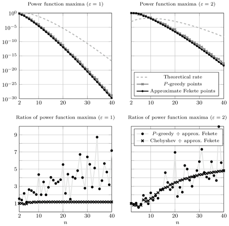
Figure 1: Top: Power function maxima $\max_{x\in[-1,1]}P_{\mathcal{X}_{n}}(x)$ approximated using a discretisation of $[-1,1]$ into 1,000 equispaced points for the approximate Fekete and $P$-greedy points of the Gaussian kernel (4.2) with $\varepsilon=1$ (left) and $\varepsilon=2$ (right). Also displayed are the (scaled) theoretical rates from Theorem 4.4. Bottom: Ratios of power function maxima for (1) $P$-greedy and approximate Fekete points and (2) Chebyshev and approximate Fekete points. These panels demonstrate that the power function for the $P$-greedy points can attain a value almost ten times that for the approximate Fekete points ($n=34$ for $\varepsilon=1$ and $n=38$ for $\varepsilon=2$) and that the approximate Fekete points are typically only marginally better than the Chebyshev points when $\varepsilon=1$ but can consistently outperform them when $\varepsilon$ is increased.

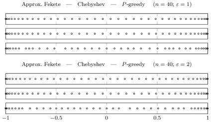
Figure 2: Approximate Fekete points (top), Chebyshev points (middle), and $P$-greedy points (bottom) on $\Omega=[-1,1]$ for the Gaussian kernel (4.2) with $\varepsilon=1$ and $\varepsilon=2$.

5.1 Power function

Figure 1 displays the maxima of power functions of the univariate Gaussian kernel (4.2) with $\varepsilon=1$ and $\varepsilon=2$ on $\Omega=[-1,1]$ for three different choices of the interpolation points:

1. The approximate Fekete points whose construction is outlined in Section 4.1.

2. The $P$-greedy points, obtained via greedy maximisation of the power function as defined in (2.9).

3. The classical Chebyshev points

   $$x_{k}=\cos\bigg{(}\frac{2k-1}{2n}\pi\bigg{)}\quad\text{ for }\quad k=1,\ldots,n$$

   which do not depend on the choice of the kernel.

The point sets are depicted in Figure 2 for $n=40$. The $P$-greedy points as well as the power function maxima were computed by discretising the interval into 1,000 equispaced points. That is, the next $P$-greedy point was always solved from

$$x_{n+1}\in\operatorname*{arg\,max}_{x\in\Omega_{h}}P_{\mathcal{X}_{n}}(x),$$ (5.1)

where $\Omega_{h}=\{-1,-1+h,\cdots,1-h,1\}$ and $h=\frac{1}{999}$, is a uniform discretisation of $[-1,1]$. The results show that the approximate Fekete points outperform the $P$-greedy points and the Chebyshev points. Given Remark 4.2 it is not surprising that the approximate Fekete points are only marginally better than the Fekete points when the relatively small value $\varepsilon=1$ is used. We also see that the approximate Fekete points are very close, but not identical, to the Chebyshev points when $\varepsilon=1$ and that they cover the domain more uniformly than the $P$-greedy points for the both values of $\varepsilon$ used.

As proved in Proposition 4.1, the approximate Fekete points are solved from a convex optimisation problem. Computing the next $P$-greedy point in (5.1) requires finding the maximum of $P_{\mathcal{X}_{n}}$ on the finite set $\Omega_{h}$, and $P_{\mathcal{X}_{n}}$ can be updated to step $n+1$ on $\Omega_{h}$ at a computational cost of $\mathcal{O}(n^{2}\mathinner{\lvert\Omega_{h}\rvert})$. On the downside, it should be noted that the power function quickly becomes numerically unstable due to severe ill-conditioning of the kernel matrix of the Gaussian kernel. The superiority of the the approximate Fekete points from computational perspective is demonstrated by our implementation which used MATLAB’s native fmincon function to efficiently compute the approximate Fekete points without domain discretisation but had to resort to costly arbitrary-precision arithmetic (mpmath library (Johansson et al., 2018) in Python) for numerically stable computation of the $P$-greedy points (arbitrary-precision arithmetic was also used to compute the power function maxima for all point sets). This makes a straightforward comparison of computational complexities of the two methods difficult.

5.2 Specific RKHS functions

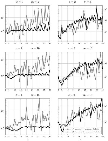
Figure 3: The ratios (5.3) of maximal errors in interpolating the function (5.2) using the kernel interpolant (2.2) based on the Gaussian kernel (4.2) with $\varepsilon=1$ (left) and $\varepsilon=2$ (right). Ratios larger than one mean that the approximate Fekete points outperform the $P$-greedy points or Chebyshev points in terms of the selected error criterion.

We use the kernel interpolant (2.2) based on the Gaussian kernel (4.2) with $\varepsilon\in\{1,2\}$ to approximate the functions

$$f_{\varepsilon,m}(x)=x^{m}\exp(x-\varepsilon^{2}x^{2})$$ (5.2)

for $m\in\{5,10,15\}$ on $\Omega=[-1,1]$. Using (4.4) and the expansion

$$f_{\varepsilon,m}(x)=x^{m}\sum_{\ell=0}^{\infty}\frac{1}{\ell!}x^{\ell}\exp(-\varepsilon^{2}x^{2})$$

we compute that

$$\mathinner{\lVert f_{\varepsilon,m}\rVert}_{\mathcal{H}_{K}(\Omega)}^{2}=\sum_{\ell=m}^{\infty}\frac{\ell!}{2^{\ell}\varepsilon^{2\ell}((\ell-m!))^{2}}=(2\varepsilon^{2})^{-m}\sum_{\ell=0}^{\infty}(2\varepsilon^{2})^{-\ell}\frac{(\ell+m)!}{(\ell!)^{2}},$$

which can be proved to converge by using, for example, the ratio test. This verifies that $f_{\varepsilon,m}\in\mathcal{H}_{K}(\Omega)$ for every $m\in\mathbf{N}$ and $\varepsilon>0$.

The results are displayed in Figure 3 in terms of the ratios of maximal interpolation errors,

$$\frac{\sup_{x\in[-1,1]}\mathinner{\lvert f_{\varepsilon,m}(x)-s_{f_{\varepsilon,m}}(x)\rvert}}{\sup_{x\in[-1,1]}\mathinner{\lvert f_{\varepsilon,m}(x)-s_{f_{\varepsilon,m}}^{*}(x)\rvert}},$$ (5.3)

where the interpolant in the numerator uses either the $P$-greedy points or the Chebyshev points and the interpolant in the denominator uses the approximate Fekete points. As in Section 5.1, the suprema were approximated using the 1,000-point equispaced discretisation of the interval and arbitrary-precision arithmetic. The results show that the approximate Fekete points fairly consistently outperform the two alternatives, particularly when the number of points and the scale parameter are large ($n\geq 15$ and $\varepsilon=2$). The results for $\varepsilon=1$ closely mirror those for the power function in Section 5.1 in that the improvement over the Chebyshev points is only marginal.

References

• Arcangéli et al. (2007) Arcangéli, R., de Silanes, M. C. L., and Torrens, J. J. (2007). An extension of a bound for functions in Sobolev spaces, with applications to $(m,s)$-spline interpolation and smoothing. Numerische Mathematik, 107(2):181–211.
• Beatson (2010) Beatson, R. (2010). Error bounds for anisotropic RBF interpolation. Journal of Approximation Theory, 162(3):512–527.
• Belhadji et al. (2019) Belhadji, A., Bardenet, R., and Chainais, P. (2019). Kernel quadrature with DPPs. In Advances in Neural Information Processing Systems, volume 32, pages 12907–12917.
• Berlinet and Thomas-Agnan (2004) Berlinet, A. and Thomas-Agnan, C. (2004). Reproducing Kernel Hilbert Spaces in Probability and Statistics. Springer.
• Bos and De Marchi (2011) Bos, L. and De Marchi, S. (2011). On optimal points for interpolation by univariate exponential functions. Dolomites Research Notes on Approximation, 4:8–12.
• Bos et al. (2010) Bos, L., De Marchi, S., Sommariva, A., and Vianello, M. (2010). Computing multivariate Fekete and Leja points by numerical linear algebra. SIAM Journal on Numerical Analysis, 48(5):1984–1999.
• Bos and Maier (2002) Bos, L. P. and Maier, U. (2002). On the asymptotics of Fekete-type points for univariate radial basis interpolation. Journal of Approximation Theory, 119(2):252–270.
• Briani et al. (2012) Briani, M., Sommariva, A., and Vianello, M. (2012). Computing Fekete and Lebesgue points: Simplex, square, disk. Journal of Computational and Applied Mathematics, 236(9):2477–2486.
• De Marchi and Schaback (2009) De Marchi, S. and Schaback, R. (2009). Nonstandard kernels and their applications. Dolomites Research Notes on Approximation, 2:16–43.
• De Marchi and Schaback (2010) De Marchi, S. and Schaback, R. (2010). Stability of kernel-based interpolation. Advances in Computational Mathematics, 32:155–161.
• De Marchi et al. (2005) De Marchi, S., Schaback, R., and Wendland, H. (2005). Near-optimal data-independent point locations for radial basis function interpolation. Advances in Computational Mathematics, 23(3):317–330.
• Fasshauer et al. (2012) Fasshauer, G., Hickernell, F., and Woźniakowski, H. (2012). On dimension-independent rates of convergence for function approximation with Gaussian kernels. SIAM Journal on Numerical Analysis, 50(1):247–271.
• Fasshauer and McCourt (2015) Fasshauer, G. and McCourt, M. (2015). Kernel-based Approximation Methods Using MATLAB. Number 19 in Interdisciplinary Mathematical Sciences. World Scientific Publishing.
• Fasshauer (2007) Fasshauer, G. E. (2007). Meshfree Approximation Methods with MATLAB. Number 6 in Interdisciplinary Mathematical Sciences. World Scientific Publishing.
• Fasshauer and McCourt (2012) Fasshauer, G. E. and McCourt, M. J. (2012). Stable evaluation of Gaussian radial basis function interpolants. SIAM Journal on Scientific Computing, 34(2):A737–A762.
• Gautier et al. (2019) Gautier, G., Bardenet, R., and Valko, M. (2019). On two ways to use determinantal point processes for Monte Carlo integration. In Advances in Neural Information Processing Systems, volume 32, pages 7768–7777.
• Johansson et al. (2018) Johansson, F. et al. (2018). mpmath: a Python library for arbitrary-precision floating-point arithmetic (version 1.10). http://mpmath.org/.
• Karvonen and Särkkä (2020) Karvonen, T. and Särkkä, S. (2020). Worst-case optimal approximation with increasingly flat Gaussian kernels. Advances in Computational Mathematics. Published online (doi.org/10.1007/s10444-020-09767-1).
• Lee et al. (2007) Lee, Y. J., Yoon, G. J., and Yoon, J. (2007). Convergence of increasingly flat radial basis interpolants to polynomial interpolants. SIAM Journal on Mathematical Analysis, 39(2):537–553.
• Minh (2010) Minh, H. Q. (2010). Some properties of Gaussian reproducing kernel Hilbert spaces and their implications for function approximation and learning theory. Constructive Approximation, 32(2):307–338.
• Müller (2009) Müller, S. (2009). Komplexität und Stabilität von kernbasierten Rekonstruktionsmethoden. PhD thesis, Institut für Numerische und Angewandte Mathematik, Georg-August-Universität Göttingen.
• Narcowich et al. (2006) Narcowich, F. J., Ward, J. D., and Wendland, H. (2006). Sobolev error estimates and a Bernstein inequality for scattered data interpolation via radial basis functions. Constructive Approximation, 24(2):175–186.
• Paulsen and Raghupathi (2016) Paulsen, V. I. and Raghupathi, M. (2016). An Introduction to the Theory of Reproducing Kernel Hilbert Spaces. Number 152 in Cambridge Studies in Advanced Mathematics. Cambridge University Press.
• Rieger and Zwicknagl (2010) Rieger, C. and Zwicknagl, B. (2010). Sampling inequalities for infinitely smooth functions, with applications to interpolation and machine learning. Advances in Computational Mathematics, 32:103–129.
• Rieger and Zwicknagl (2014) Rieger, C. and Zwicknagl, B. (2014). Improved exponential convergence rates by oversampling near the boundary. Constructive Approximation, 39(2):323–341.
• Robbins (1955) Robbins, H. (1955). A remark on Stirling’s formula. The American Mathematical Monthly, 62(1):26–29.
• Santin and Haasdonk (2017) Santin, G. and Haasdonk, B. (2017). Convergence rate of the data-independent $P$-greedy algorithm in kernel-based approximation. Dolomites Research Notes on Approximation, 10:68–78.
• Schaback (1999) Schaback, R. (1999). Improved error bounds for scattered data interpolation by radial basis functions. Mathematics of Computation, 68(225):201–216.
• Schaback (2000) Schaback, R. (2000). A unified theory of radial basis functions: Native Hilbert spaces for radial basis functions II. Journal of Computational and Applied Mathematics, 121(1–2):165–177.
• Schaback (2005) Schaback, R. (2005). Multivariate interpolation by polynomials and radial basis functions. Constructive Approximation, 21(3):293–317.
• Schaback (2018) Schaback, R. (2018). Superconvergence of kernel-based interpolation. Journal of Approximation Theory, 235:1–19.
• Schaback and Wendland (2000) Schaback, R. and Wendland, H. (2000). Adaptive greedy techniques for approximate solution of large RBF systems. Numerical Algorithms, 24(3):239–254.
• Sloan and Woźniakowski (2018) Sloan, I. H. and Woźniakowski, H. (2018). Multivariate approximation for analytic functions with Gaussian kernels. Journal of Complexity, 45:1–21.
• Steinwart et al. (2006) Steinwart, I., Hush, D., and Scovel, C. (2006). An explicit description of the reproducing kernel Hilbert spaces of Gaussian RBF kernels. IEEE Transactions on Information Theory, 52(10):4635–4643.
• Sun (2005) Sun, H. (2005). Mercer theorem for RKHS on noncompact sets. Journal of Complexity, 21(3):337–349.
• Tanaka (2019) Tanaka, K. (2019). Generation of point sets by convex optimization for interpolation in reproducing kernel Hilbert spaces. Numerical Algorithms. Published online (doi:10.1007/s11075-019-00792-w).
• Tanaka and Sugihara (2019) Tanaka, K. and Sugihara, M. (2019). Design of accurate formulas for approximating functions in weighted Hardy spaces by discrete energy minimization. IMA Journal of Numerical Analysis, 39(4):1957–1984.
• Wendland (2005) Wendland, H. (2005). Scattered Data Approximation. Number 17 in Cambridge Monographs on Applied and Computational Mathematics. Cambridge University Press.
• Wendland and Rieger (2005) Wendland, H. and Rieger, C. (2005). Approximate interpolation with applications to selecting smoothing parameters. Numerische Mathematik, 101(4):729–748.
• Wirtz and Haasdonk (2013) Wirtz, D. and Haasdonk, B. (2013). A vectorial kernel orthogonal greedy algorithm. Dolomites Research Notes on Approximation, 6:83–100.