Regularity versus smoothness of measures

Abstract

The Assouad and lower dimensions and dimension spectra quantify the regularity of a measure by considering the relative measure of concentric balls. On the other hand, one can quantify the smoothness of an absolutely continuous measure by considering the $L^{p}$ norms of its density. We establish sharp relationships between these two notions. Roughly speaking, we show that smooth measures must be regular, but that regular measures need not be smooth.

Mathematics Subject Classification 2010: primary: 28A80; secondary: 37C45.

Key words and phrases: Assouad dimension, Assouad spectrum, lower dimension, lower spectrum, $L^{p}$-spaces.

1 Introduction and preliminaries.

1.1 Assouad type dimensions and spectra of measures.

The Assouad and lower dimensions of measures, also known as the regularity dimensions, are important notions in dimension theory and geometric measure theory. They capture extremal scaling behaviour of measures by considering the relative measure of concentric balls and have a strong connection to doubling properties. A fundamental result is that a measure has finite Assouad dimension if and only if it is doubling and that a measure has positive lower dimensions if and only if it is inverse doubling, see e.g. [KL17, KLV13]. As such, these dimensions quantify the regularity of a measure. The Assouad and lower spectrum provide a more nuanced analysis along these lines by fixing the relationship between the radii of the concentric balls according to a parameter $\theta\in(0,1)$ which is then varied to produce the spectra. Motivated by progress on Assouad type dimensions and spectra for sets, the analogues for measure were investigated in [KL17, KLV13, FH18, HHT19, HT18].

Throughout we assume that $\mu$ is a Borel probability measure on a compact metric space $(X,d)$. These assumptions can be weakened in places but we make them for expository reasons. We write $\operatorname{supp}\mu$ for the support of $\mu$. The Assouad dimension of $\mu$ is defined as

$$\operatorname{\dim_{\mathrm{A}}}\mu\ =\ \inf\Bigg{\{}\alpha\ :\ (\exists\,C>0)\,(\forall\,0<r<R<1)\,(\forall x\in\operatorname{supp}\mu),\ \frac{\mu(B(x,R))}{\mu(B(x,r))}\ \leqslant\ C\bigg{(}\frac{R}{r}\bigg{)}^{\alpha}\Bigg{\}}.$$

Its dual, the lower dimension, is defined analogously as

$$\operatorname{\dim_{\mathrm{L}}}\mu\ =\ \sup\Bigg{\{}\alpha\ :\ (\exists\,C>0)\,(\forall\,0<r<R<1)\,(\forall x\in\operatorname{supp}\mu),\ \frac{\mu(B(x,R))}{\mu(B(x,r))}\ \geqslant\ C\bigg{(}\frac{R}{r}\bigg{)}^{\alpha}\Bigg{\}}.$$

The Assouad spectrum is the function defined by

$$\theta\ \mapsto\ \operatorname{{\dim}_{\mathrm{A}}^{\theta}}\mu\ =\ \inf\bigg{\{}\alpha\ :\ (\exists C>0)\,(\forall 0<R<1)\,(\forall x\in\operatorname{supp}\mu),\\ \frac{\mu(B(x,R))}{\mu(B(x,R^{1/\theta}))}\ \leqslant\ C\left(\frac{R}{R^{1/\theta}}\right)^{\alpha}\bigg{\}},$$

where $\theta$ varies over $(0,1)$. The related quasi-Assouad dimension can be defined by

$$\operatorname{{\dim}_{\mathrm{qA}}}\mu\ =\ \lim_{\theta\to 1}\operatorname{{\dim}_{\mathrm{A}}^{\theta}}\mu$$

when it is finite. This is not the original definition, which stems from [LX16], but a convenient equivalent formulation which was established in [HT18, Proposition 6.2], following [FHHTY18]. Similarly, the lower spectrum is defined by

$$\theta\ \mapsto\ \operatorname{{\dim}_{\mathrm{L}}^{\theta}}\mu\ =\ \sup\bigg{\{}\alpha\ :\ (\exists C>0)\,(\forall 0<R<1)\,(\forall x\in\operatorname{supp}\mu),\\ \frac{\mu(B(x,R))}{\mu(B(x,R^{1/\theta}))}\ \geqslant\ C\left(\frac{R}{R^{1/\theta}}\right)^{\alpha}\bigg{\}}$$

and the quasi-lower dimension by

$$\operatorname{{\dim}_{\mathrm{qL}}}\mu\ =\ \lim_{\theta\to 1}\operatorname{{\dim}_{\mathrm{L}}^{\theta}}\mu.$$

The Assouad and lower spectra (of sets) were defined in [FY18] and are designed to extract finer geometric information than the Assouad, lower, and box-counting dimensions considered in isolation. See the survey [F19] for more on this approach to dimension theory.

These Assouad-type dimensions and spectra are related by

$$\operatorname{\dim_{\mathrm{L}}}\mu\leqslant\operatorname{{\dim}_{\mathrm{qL}}}\mu\leqslant\operatorname{{\dim}_{\mathrm{L}}^{\theta}}\mu \leqslant\inf_{x\in\operatorname{supp}\mu}\underline{\dim}_{\mathrm{loc}}\mu(x)$$

$$\leqslant\sup_{x\in\operatorname{supp}\mu}\overline{\dim}_{\mathrm{loc}}\mu(x)\leqslant\operatorname{{\dim}_{\mathrm{A}}^{\theta}}\mu\leqslant\operatorname{{\dim}_{\mathrm{qA}}}\mu\leqslant\operatorname{\dim_{\mathrm{A}}}\mu,$$

where $\overline{\dim}_{\mathrm{loc}}\mu(x)$ and $\underline{\dim}_{\mathrm{loc}}\mu(x)$ are the upper and lower local dimensions of $\mu$ at a point $x$. We do not use the local dimensions but mention them here to emphasise that the Assouad and lower dimensions are extremal, since most familiar notions of dimensions for measures lie in between the infimal and supremal lower dimensions, e.g. the Hausdorff dimension. For more information, including basic properties, concerning Assouad-type dimensions of measures, see [FH18, HHT19, HT18, KL17, KLV13].

1.2 $L^{p}$ properties of measures.

A probability measure $\mu$ supported on a compact subset $X\subset\mathbb{R}^{d}$ is absolutely continuous (with respect to the Lebesgue measure), if all Lebesgue null sets are given zero $\mu$ measure. In particular, this means that there is a Lebesgue integrable function $f$, the density or Radon-Nikodym derivative, such that

$$\mu(E)=\int_{E}f(x)\,dx$$

for all Borel sets $E$. Given $p\geqslant 1$, the space $L^{p}(X)$ is defined to consist of all integrable functions $g$ such that

$$\|g\|_{p}:=\left(\int_{X}g(x)^{p}\,dx\right)^{1/p}<\infty.$$

The space $L^{\infty}(X)$ denotes the space of essentially bounded functions. In a slight abuse of notation, we say $\mu\in L^{p}(X)$ if $\mu$ is absolutely continuous with density $f\in L^{p}$. Given an absolutely continuous measure $\mu$, we can thus understand how smooth $\mu$ is by determining precisely for which $p$ we have $\mu\in L^{p}(X)$. Since we assume $\mu$ is compactly supported, $\mu\in L^{p_{2}}(X)$ implies $\mu\in L^{p_{1}}(X)$ for all $1\leqslant p_{1}\leqslant p_{2}\leqslant\infty$ and therefore it is harder for the $\mu$ to be in $L^{p}(X)$ as $p$ increases. We think of measures being smoother if they lie in $L^{p}(X)$ for larger $p$ and $L^{\infty}(X)$ as consisting of the smoothest measures possible, according to this analysis.

One can consider absolute continuity with respect to arbitrary reference measures in place of the Lebesgue measure. Much of our work would also apply in this setting, but we focus on $X=[a,b]\subset\operatorname{\mathbb{R}}$ with the Lebesgue measure as the reference measure and write $L^{p}$ instead of $L^{p}([a,b])$. Our results also easily extend to higher dimensions, that is, when the reference measure is $d$-dimensional Lebesgue measure. We focus on the 1-dimensional case with Lebesgue measure as the reference measure since this is the most natural and important case and also to simplify our exposition.

It will also be useful to consider ‘inverse $L^{p}$ spaces’. We write $f\in L^{-p}$ if the set $E=\{x\in X:f(x)=0\}\subset X$ is of Lebesgue measure zero and

$$\left(\int_{X\setminus E}1/f(x)^{p}dx\right)^{1/p}<\infty.$$

Analogous to above we write $\mu\in L^{-p}$ if $\mu$ is absolutely continuous with density in $L^{-p}$.

2 Main results: smoothness versus regularity.

The objective of this article is to investigate the relationships between regularity and smoothness, as described by Assouad type dimensions and spectra and $L^{p}$ properties, respectively.

First, we remark that for an absolutely continuous measure $\mu$, the condition that $\mu\in L^{p}$ does not guarantee that $\operatorname{\dim_{\mathrm{L}}}\mu>0$ or $\operatorname{\dim_{\mathrm{A}}}\mu<\infty$. All one can conclude is that $0\leqslant\operatorname{\dim_{\mathrm{L}}}\mu\leqslant 1\leqslant\operatorname{\dim_{\mathrm{A}}}\mu\leqslant\infty$. Even the strong assumption that the density of a measure is bounded, does not guarantee a measure is doubling, take for instance the density on $[-1,1]$ defined by

$$f(x)=\begin{cases}2^{-k}&\text{ if }2^{-k}\leqslant x<2^{-k+1}\\ \frac{2}{3}&\text{ otherwise}\end{cases}$$

for $k\in\operatorname{\mathbb{N}}$. One can check that $\int_{-1}^{1}f(x)dx=1$ and thus $\mu$ is a probability measure. The ball $B(2^{-k},2^{-k})$ has measure $4/3\cdot 4^{-k}$, whereas $\mu(B(2^{-k},2^{-k+1}))=2/3\cdot 2^{-k}+4/3\cdot 4^{-k+1}$ and therefore

$$\frac{\mu(B(2^{-k},2^{-k+1}))}{\mu(B(2^{-k},2^{-k}))}\ \geqslant\ 2^{k-1}\to\infty.$$

Therefore, the measure is not doubling and, in particular, $\operatorname{\dim_{\mathrm{A}}}\mu=\infty$. Bounded density is also not enough to say something about the quasi-Assouad dimension or Assouad spectrum, see below. It turns out we need to be able to control the density from both sides in order to get good estimates for the Assouad type dimensions. Our main result establishes a sharp correspondence along these lines.

Theorem 2.1.

Suppose $p_{1},p_{2}\in[1,\infty]$ are such that $\mu\in L^{p_{1}}\cap L^{-p_{2}}$. If $p_{1},p_{2}<\infty$, then

$$\operatorname{{\dim}_{\mathrm{A}}^{\theta}}\mu\leqslant 1+\frac{p_{1}+\theta p_{2}}{p_{1}p_{2}(1-\theta)}\quad\text{and}\quad\operatorname{{\dim}_{\mathrm{L}}^{\theta}}\mu\geqslant 1-\frac{\theta p_{1}+p_{2}}{p_{1}p_{2}(1-\theta)}.$$ (2.1)

If $\mu\in L^{\infty}\cap L^{-\infty}$, then $\mu$ is 1-Ahlfors regular and $\operatorname{\dim_{\mathrm{A}}}\mu=\operatorname{\dim_{\mathrm{L}}}\mu=1$ and if $\mu\in L^{p_{1}}\cap L^{-\infty}$ or $\mu\in L^{\infty}\cap L^{-p_{2}}$, then one can obtain bounds by taking the limit as $p_{1}$ or $p_{2}$ tends to infinity in (2.1). Moreover, all of these bounds are sharp.

The fact that these bounds above are sharp shows that knowledge of $L^{p}$-smoothness and inverse $L^{p}$-smoothness are not sufficient to give bounds on the regularity as measured by the quasi-Assouad and Assouad dimensions, or the quasi-lower and lower dimensions. This is seen by letting $\theta\to 1$.

2.1 Proof of Theorem 2.1.

Throughout the rest of the paper we write $A\lesssim B$ to mean there exists a uniform constant $c>0$ such that $A\leqslant cB$. Similarly, we write $A\gtrsim B$ to mean $B\lesssim A$ and $A\approx B$ if $A\lesssim B$ and $A\gtrsim B$.

2.1.1 Establishing the bounds.

The proof uses Hölder’s inequality and the reverse Hölder inequality. That is, for all $p>1$ and $q$ such that $1/p+1/q=1$ and measurable functions $f,g$ we have

$$\lVert fg\rVert_{1}\leqslant\lVert f\rVert_{p}\lVert g\rVert_{q}\quad\text{and}\quad\lVert fg\rVert_{1}\geqslant\lVert f\rVert_{-p}\lVert g\rVert_{p/(p+1)},$$

where for the latter we also require that $f(x)\neq 0$ for almost every $x$. We note that $\lVert f\rVert_{-p}$ and $\lVert g\rVert_{p/(p+1)}$ are not norms but convenient notation for

$$\lVert f\rVert_{-p}=\left(\int f(x)^{-p}dx\right)^{-1/p}\quad\text{and}\qquad\lVert g\rVert_{p/(p+1)}=\left(\int f(x)^{p/(p+1)}dx\right)^{(p+1)/p},$$

respectively. We use the above inequalities to estimate

$$\frac{\mu(B(x,R))}{\mu(B(x,r))}=\frac{\lVert f\cdot\chi_{B(x,R)}\rVert_{1}}{\lVert f\cdot\chi_{B(x,R)}\rVert_{1}},$$ (2.2)

where $f$ is the density of $\mu$ and $\chi_{A}$ is the indicator function associated with a set $A$.

Fix $\theta\in(0,1)$ and let $r=R^{1/\theta}$. Write $q_{1}\in(1,\infty)$ for the Hölder conjugate of $p_{1}$, that is the unique value satisfying $1/p_{1}+1/q_{1}=1$. Noting that $\frac{\lVert f\rVert_{p_{1}}}{\lVert f\rVert_{-p_{2}}}\in(0,\infty)$ is a constant independent of $R$, we can bound (2.2) from above by

$$\frac{\mu(B(x,R))}{\mu(B(x,r))}\leqslant\frac{\lVert f\rVert_{p_{1}}\lVert\chi_{B(x,R)}\rVert_{q_{1}}}{\lVert f\rVert_{-p_{2}}\lVert\chi_{B(x,r)}\rVert_{p_{2}/(1+p_{2})}} \lesssim\frac{\left(\int\chi_{B(x,R)}^{q_{1}}d\mu\right)^{1/q_{1}}}{\left(\int\chi_{B(x,r)}^{p_{2}/(1+p_{2})}d\mu\right)^{1+1/p_{2}}}$$

$$\lesssim\dfrac{R^{1-1/p_{1}}}{r^{1+1/p_{2}}}$$

$$=\left(\frac{R}{r}\right)^{\frac{1-1/p_{1}-1/\theta(1+1/p_{2})}{1-1/\theta}}.$$

Therefore,

$$\operatorname{{\dim}_{\mathrm{A}}^{\theta}}\mu\leqslant\frac{1-1/p_{1}-1/\theta(1+1/p_{2})}{1-1/\theta}=1+\frac{p_{1}+\theta p_{2}}{p_{1}p_{2}(1-\theta)},$$

as required.

We can bound (2.2) from below similarly by

$$\frac{\mu(B(x,R))}{\mu(B(x,r))}\geqslant\frac{\lVert f\rVert_{-p_{2}}\lVert\chi_{B(x,R)}\rVert_{p_{2}/(1+p_{2})}}{\lVert f\rVert_{p_{1}}\lVert\chi_{B(x,r)}\rVert_{q_{1}}} \gtrsim\dfrac{R^{1+1/p_{2}}}{r^{1-1/p_{1}}}$$

$$=\left(\frac{R}{r}\right)^{\frac{1+1/p_{2}-1/\theta(1-1/p_{1})}{1-1/\theta}}.$$

Therefore,

$$\operatorname{{\dim}_{\mathrm{L}}^{\theta}}\mu\geqslant\frac{1+1/p_{2}-1/\theta(1-1/p_{1})}{1-1/\theta}=1-\frac{\theta p_{1}+p_{2}}{p_{1}p_{2}(1-\theta)},$$

as required.

Finally, note that if $\mu\in L^{\infty}\cap L^{-\infty}$, then

$$\|f\|_{-\infty}\cdot r\leqslant\mu(B(x,r))\leqslant\|f\|_{\infty}\cdot r$$

for all $x$ in the support of $\mu$ and all $r\in(0,1)$. Therefore $\mu$ is $1$-Ahlfors regular. The fact that the estimates are sharp is proved in the following subsections.

2.1.2 Sharpness for the Assouad spectrum.

The following lemma shows that the estimate for the Assouad spectrum in Theorem 2.1 is sharp for all $\theta\in(0,1)$. Moreover, this shows that a measure can belong to $L^{p_{1}}\cap L^{-p_{2}}$ whilst being non-doubling (that is, $\operatorname{\dim_{\mathrm{A}}}\mu=\infty$) and even have infinite quasi-Assouad dimension.

Lemma 2.2.

The bounds on the Assouad spectrum in Theorem 2.1 are sharp. That is, given $p_{1},p_{2}\in(1,\infty]$ there exists a probability measure $\mu$ such that $\mu\in L^{p_{1}^{\prime}}\cap L^{-p_{2}^{\prime}}$ for all $p_{1}^{\prime}<p_{1}$ and $p_{2}^{\prime}<p_{2}$, and

$$\operatorname{{\dim}_{\mathrm{A}}^{\theta}}\mu=1+\frac{p_{1}+\theta p_{2}}{p_{1}p_{2}(1-\theta)}$$

for all $\theta\in(0,1)$.

Proof.

Let $p_{1},p_{2}\in(1,\infty]$ and let $\mu$ be the probability measure supported on $[-1,1]$ with density

$$f(x)=\begin{cases}Cx^{-1/p_{1}}&0<x\leqslant 1\\ C(-x)^{1/p_{2}}&-1\leqslant x\leqslant 0\end{cases},$$

where $C$ is chosen such that $\int f(x)dx=1$, see Figure 1. We adopt the natural convention that $1/\infty=0$. It is easily checked that $f\in L^{p_{1}^{\prime}}\cap L^{-p_{2}^{\prime}}$ for $p_{1}^{\prime}<p_{1}$ and $p_{2}^{\prime}<p_{2}$, but that $f\notin L^{p_{1}^{\prime\prime}}\cap L^{-p_{2}^{\prime\prime}}$ if either $p_{1}^{\prime\prime}=p_{1}$ or $p_{2}^{\prime\prime}=p_{2}$.

In order to bound the Assouad spectrum from below it suffices to find points such that the relative measure of balls centred at that point is large. To this end, let $R\in(0,1)$, $r=R^{1/\theta}$ and consider the point $-r$, where we find

$$\frac{\mu(B(-r,R))}{\mu(B(-r,r))}=\frac{\int_{-r-R}^{0}(-x)^{1/p_{2}}dx+\int_{0}^{R-r}x^{-1/p_{1}}dx}{\int_{-2r}^{0}(-x)^{1/p_{2}}dx} \approx\frac{(R+r)^{1+1/p_{2}}+(R-r)^{1-1/p_{1}}}{r^{1+1/p_{2}}}$$

$$\gtrsim\frac{R^{1-1/p_{1}}}{r^{1+1/p_{2}}}$$

$$\gtrsim\left(\frac{R}{r}\right)^{\frac{1-1/p_{1}-1/\theta(1+1/p_{2})}{1-1/\theta}}.$$

This shows that

$$\operatorname{{\dim}_{\mathrm{A}}^{\theta}}\mu\geqslant\frac{1-1/p_{1}-1/\theta(1+1/p_{2})}{1-1/\theta}=1+\frac{p_{1}+\theta p_{2}}{p_{1}p_{2}(1-\theta)}$$

and

$$\operatorname{{\dim}_{\mathrm{qA}}}\mu=\operatorname{\dim_{\mathrm{A}}}\mu=\infty.$$

In fact, applying Theorem 2.1 to this example we see that

$$\operatorname{{\dim}_{\mathrm{A}}^{\theta}}\mu=1+\frac{p_{1}+\theta p_{2}}{p_{1}p_{2}(1-\theta)}$$

for all $\theta\in(0,1)$. ∎

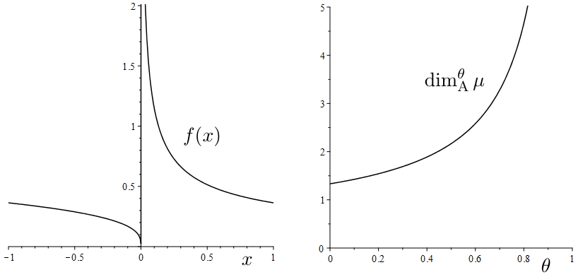
Figure 1: A sharp example for the Assouad spectrum, with $p_{1}=2$, $p_{2}=3$ and $C=4/11$. The density is plotted on the left and the Assouad spectrum is plotted on the right.

2.1.3 Sharpness for the lower spectrum.

The following lemma shows that the estimate for the lower spectrum in Theorem 2.1 is sharp for all $\theta\in(0,1)$. Moreover, this shows that a measure can belong to $L^{p_{1}}\cap L^{-p_{2}}$ whilst being non-inverse doubling (that is, $\operatorname{\dim_{\mathrm{L}}}\mu=0$) and even have quasi-lower dimension equal to 0.

Lemma 2.3.

The bounds on the lower spectrum in Theorem 2.1 are sharp. That is, given $p_{1},p_{2}\in(1,\infty]$ there exists a probability measure $\mu$ such that $\mu\in L^{p_{1}^{\prime}}\cap L^{-p_{2}^{\prime}}$ for all $p_{1}^{\prime}<p_{1}$ and $p_{2}^{\prime}<p_{2}$, and

$$\operatorname{{\dim}_{\mathrm{L}}^{\theta}}\mu=\max\left\{1-\frac{\theta p_{1}+p_{2}}{p_{1}p_{2}(1-\theta)},\ 0\right\}$$

for all $\theta\in(0,1)$.

Proof.

Let $p_{1},p_{2}\in(1,\infty]$ and $\theta_{i}$ ($i\geqslant 1$) be an enumeration of $\operatorname{\mathbb{Q}}\cap(0,1)$ such that for every rational $q\in\operatorname{\mathbb{Q}}\cap(0,1)$ there are infinitely many $i\in\operatorname{\mathbb{N}}$ such that $\theta_{i}=q$. Let $x_{i}=2^{-i}+2^{-(i+1)}$ and $\mu$ be the probability measure supported on $[0,1]$ with density

$$f(x)=\begin{cases}C2^{i/(\theta_{i}p_{1})}&x\in B(x_{i},2^{-(i+1)/\theta_{i}})\\ C2^{-i/p_{2}}&x\in B(x_{i},2^{-(i+1)})\setminus B(x_{i},2^{-(i+1)/\theta_{i}})\\ 0&\textup{otherwise}\end{cases},$$

where $C$ is chosen such that $\int f(x)dx=1$ and the balls are assumed to be open, see Figure 2. We adopt the natural convention that $1/\infty=0$. Moreover, by construction, the balls $B(x_{i},2^{-(i+1)})$ are pairwise disjoint subsets of $[0,1]$ and so $f$ is well-defined.

There exists a constant $c>0$ such that $c^{-1}x^{1/p_{2}}\leqslant f(x)$ and therefore $\mu\in L^{-p_{2}^{\prime}}$ for $p_{2}^{\prime}<p_{2}$. Moreover, for $p_{1}^{\prime}<p_{1}$ we have

$$\int f(x)^{p_{1}^{\prime}}dx\lesssim\sum_{i}2^{ip_{1}^{\prime}/(\theta_{i}p_{1})}2^{-i/\theta_{i}}\leqslant\sum_{i}2^{i(p_{1}^{\prime}/p_{1}-1)}<\infty$$

and therefore $\mu\in L^{p_{1}^{\prime}}$.

In order to bound the lower spectrum from above it suffices to find points such that the relative measure of balls centred at that point is small. To this end, fix $\theta\in\operatorname{\mathbb{Q}}\cap(0,1)$ and a subsequence of the $\theta_{i}$, which we denote by $\theta_{k}$, such that $\theta_{k}=\theta$ for all $k$. Along this sequence, let $R_{k}=2^{-(k+1)}$, $r_{k}=R_{k}^{1/\theta}$ and consider the points $x_{k}=2^{-k}+2^{-(k+1)}$, where we find

$$\frac{\mu(B(x_{k},R_{k}))}{\mu(B(x_{k},r_{k}))}\lesssim\frac{r_{k}2^{k/(\theta p_{1})}+R_{k}2^{-k/p_{2}}}{r_{k}2^{k/(\theta p_{1})}}\approx\frac{R_{k}^{1/\theta-1/(\theta p_{1})}+R_{k}^{1+1/p_{2}}}{R_{k}^{1/\theta-1/(\theta p_{1})}}.$$ (2.3)

Provided $1/\theta-1/(\theta p_{1})>1+1/p_{2}$ this gives an upper bound of

$$\lesssim\frac{R_{k}^{1+1/p_{2}}}{R_{k}^{1/\theta-1/(\theta p_{1})}}=\left(\frac{R_{k}}{r_{k}}\right)^{\frac{1+1/p_{2}-1/\theta+1/(\theta p_{1})}{1-1/\theta}}$$

for (2.3). This shows

$$\operatorname{{\dim}_{\mathrm{L}}^{\theta}}\mu\leqslant\frac{1+1/p_{2}-1/\theta+1/(\theta p_{1})}{1-1/\theta}=1-\frac{\theta p_{1}+p_{2}}{p_{1}p_{2}(1-\theta)}.$$

On the other hand, if $1/\theta-1/(\theta p_{1})\leqslant 1+1/p_{2}$, this gives an upper bound of $\lesssim 1$ for (2.3), which implies $\operatorname{\dim_{\mathrm{L}}}\mu\leqslant 0$. Putting these two cases together we get

$$\operatorname{{\dim}_{\mathrm{L}}^{\theta}}\mu\leqslant\max\left\{1-\frac{\theta p_{1}+p_{2}}{p_{1}p_{2}(1-\theta)},\ 0\right\}$$

for all rational $\theta\in(0,1)$. Since the lower spectrum is continuous in $\theta\in(0,1)$, we therefore conclude this upper bound for all $\theta\in(0,1)$. Moreover, we get

$$\operatorname{{\dim}_{\mathrm{qL}}}\mu=\operatorname{\dim_{\mathrm{L}}}\mu=0.$$

In fact, applying Theorem 2.1 we get

$$\operatorname{{\dim}_{\mathrm{L}}^{\theta}}\mu=\max\left\{1-\frac{\theta p_{1}+p_{2}}{p_{1}p_{2}(1-\theta)},\ 0\right\}$$

for all $\theta\in(0,1)$.∎

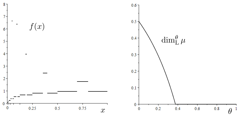
Figure 2: A sharp example for the lower spectrum, with $p_{1}=2$ and $p_{2}=3$. The density is plotted on the left and the Assouad spectrum is plotted on the right. The density is not drawn to scale and is mostly for illustrative purposes.

3 Piecewise monotonic densities.

Given that the Assouad and lower spectra are dual notions, it is quite striking how different the examples in the previous section are. In particular, the measure exhibiting sharpness of the Assouad spectrum bound in Theorem 2.1 has a piecewise monotonic density (Section 2.1.2 and Figure 1), whereas the measure exhibiting sharpness of the lower spectrum bound does not, and is rather more complicated to construct (Section 2.1.3 and Figure 2). This turns out to be no coincidence. Here, and in what follows, piecewise means with finitely many pieces.

Theorem 3.1.

Suppose $p_{1},p_{2}\in[1,\infty)$ are such that $\mu\in L^{p_{1}}\cap L^{-p_{2}}$. If $\mu$ has a monotonic density, then

$$\operatorname{{\dim}_{\mathrm{A}}^{\theta}}\mu\leqslant\max\left\{1+\frac{1}{p_{2}(1-\theta)},\ 1+\frac{\theta}{p_{1}(1-\theta)}\right\}$$

and

$$\operatorname{{\dim}_{\mathrm{L}}^{\theta}}\mu\geqslant\min\left\{1-\frac{\theta}{p_{2}(1-\theta)},\ 1-\frac{1}{p_{1}(1-\theta)}\right\}.$$

If $\mu$ has a piecewise monotonic density, then

$$\operatorname{{\dim}_{\mathrm{A}}^{\theta}}\mu\leqslant 1+\frac{p_{1}+\theta p_{2}}{p_{1}p_{2}(1-\theta)}$$

and

$$\operatorname{{\dim}_{\mathrm{L}}^{\theta}}\mu\geqslant\min\left\{1-\frac{\theta}{p_{2}(1-\theta)},\ 1-\frac{1}{p_{1}(1-\theta)}\right\}.$$

Moreover, all of these bounds are sharp.

3.1 Proof of Theorem 3.1.

3.1.1 Establishing the bounds.

We begin with the case when $\mu$ has a monotonic density, which we denote by $f$. It follows that for all sufficiently small $R>0$ (depending on $f$) and all $x$, at least one of the following is satisfied:

1. $f$ is bounded above by 2 on $B(x,R)$

2. $f$ is bounded below by 2 on $B(x,R)$

3. $f$ is bounded above by 3 and below by 1 on $B(x,R)$

In each of these cases we follow the proof of Theorem 2.1 but we can obtain better estimates. In Case 1 we have

$$\frac{\mu(B(x,R))}{\mu(B(x,r))}\leqslant\frac{2\lVert\chi_{B(x,R)}\rVert_{1}}{\lVert f\rVert_{-p_{2}}\lVert\chi_{B(x,r)}\rVert_{p_{2}/(1+p_{2})}}\lesssim\frac{R}{r^{1+1/p_{2}}}=\left(\frac{R}{r}\right)^{\frac{1-1/\theta(1+1/p_{2})}{1-1/\theta}},$$

in Case 2 we have

$$\frac{\mu(B(x,R))}{\mu(B(x,r))}\leqslant\frac{\lVert f\rVert_{p_{1}}\lVert\chi_{B(x,R)}\rVert_{q_{1}}}{(1/2)\lVert\chi_{B(x,r)}\rVert_{1}}\lesssim\dfrac{R^{1-1/p_{1}}}{r}\\ =\left(\frac{R}{r}\right)^{\frac{1-1/p_{1}-1/\theta}{1-1/\theta}},$$

and in Case 3

$$\frac{\mu(B(x,R))}{\mu(B(x,r))}\leqslant\frac{3\lVert\chi_{B(x,R)}\rVert_{1}}{\lVert\chi_{B(x,r)}\rVert_{1}}\lesssim\frac{R}{r}.$$

The estimate in the theorem follows. The lower spectrum case is similar and omitted.

We now consider the case when $\mu$ has a piecewise monotonic density, which we denote by $f$. This is similar to the monotonic case, but an interesting phenomenon happens allowing us to improve the general estimate for the lower spectrum in a way we cannot for the Assouad spectrum.

The upper bound for the Assouad spectrum is provided by Theorem 2.1 and the fact that this is sharp is shown by the example in Section 2.1.2. Therefore we may consider only the lower spectrum. Since $f$ is piecewise monotonic it follows that for all sufficiently small $R>0$ (depending on $f$) and all $x$, at least one of the following is satisfied:

1. $f$ is bounded above by 2 on $B(x,R)$

2. $f$ is bounded below by 2 on $B(x,R)$

3. $f$ is bounded above by 3 and below by 1 on $B(x,R)$

4. $B(x,R)$ can be written as a disjoint union of two intervals $I_{1}\cup I_{2}$ such that $f$ is bounded above by 1 on $I_{1}$ and below by $1$ on $I_{2}$. One of the intervals $I_{1}$ or $I_{2}$ may be empty and they can be closed, open or half open.

In each of these cases we follow the proof of Theorem 2.1 but we can obtain better estimates. Cases 1-3 are covered above. In Case 4, either $B(x,r)\subseteq I_{1}$ or not. If $B(x,r)\subseteq I_{1}$, then

$$\frac{\mu(B(x,R))}{\mu(B(x,r))}\geqslant\frac{\lVert f\rVert_{-p_{2}}\lVert\chi_{B(x,R)}\rVert_{p_{2}/(1+p_{2})}}{\lVert\chi_{B(x,r)}\rVert_{1}}\gtrsim\dfrac{R^{1+1/p_{2}}}{r}=\left(\frac{R}{r}\right)^{\frac{1+1/p_{2}-1/\theta}{1-1/\theta}}.$$

If $B(x,r)$ is not completely contained inside $I_{1}$, then there must be an interval of length $R-r\gtrsim R$ contained in $I_{2}$ in which case

$$\frac{\mu(B(x,R))}{\mu(B(x,r))}\geqslant\frac{\mu(I_{2})}{\mu(B(x,r))}\geqslant\frac{\lVert\chi_{I_{2}}\rVert_{1}}{\lVert f\rVert_{p_{1}}\lVert\chi_{B(x,r)}\rVert_{q_{1}}}\gtrsim\dfrac{R}{r^{1-1/p_{1}}}=\left(\frac{R}{r}\right)^{\frac{1-1/\theta(1-1/p_{1})}{1-1/\theta}}.$$

The estimate in the theorem follows.

3.1.2 Sharpness.

It remains to show that the estimates in Theorem 3.1 are sharp. This requires only one further example, where $\mu$ is the measure on $[0,2]$ with density

$$f(x)=\begin{cases}Cx^{-1/p_{1}}&0<x\leqslant 1\\ C(2-x)^{1/p_{2}}&1<x\leqslant 2\end{cases},$$

where $C$ is chosen such that $\int f(x)dx=1$. Minor adaptations of the above arguments yield

$$\operatorname{{\dim}_{\mathrm{A}}^{\theta}}\mu=\max\left\{1+\frac{1}{p_{2}(1-\theta)},\ 1+\frac{\theta}{p_{1}(1-\theta)}\right\}$$

and

$$\operatorname{{\dim}_{\mathrm{L}}^{\theta}}\mu=\max\left\{\min\left\{1-\frac{\theta}{p_{2}(1-\theta)},\ 1-\frac{1}{p_{1}(1-\theta)}\right\},\ 0\right\}.$$

as required.

Note that for this family of sharp examples, the Assouad spectrum will exhibit a phase transition at $\theta=p_{1}/p_{2}$ provided $p_{1}<p_{2}$ and the lower spectrum is constantly equal to 0 for

$$\theta>\min\left\{\frac{p_{2}}{1+p_{2}},\frac{p_{1}-1}{p_{1}}\right\}.$$

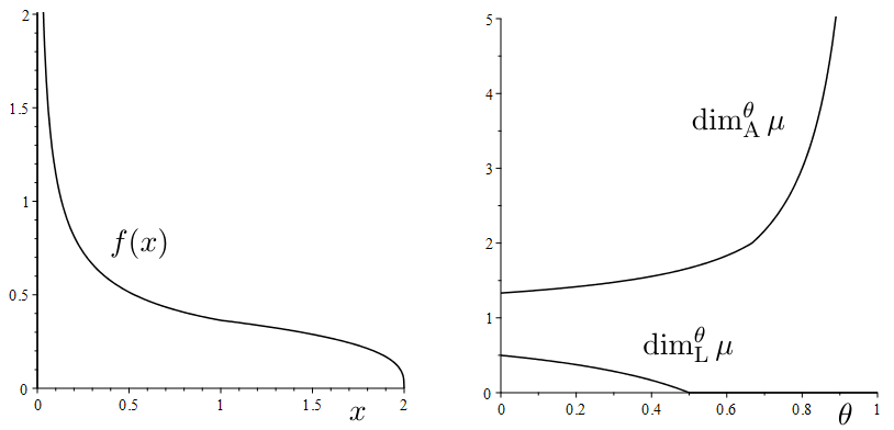
Figure 3: A sharp example in the monotonic case, where $p_{1}=2,p_{2}=3$ and $C=4/11$. The density is plotted on the left and the Assouad and lower spectra are plotted on the right. Note that the Assouad spectrum has a phase transition at $\theta=2/3$ and the lower spectrum has a phase transition at $\theta=1/2$.

4 A relationship in the opposite direction?

So far we have proved results of the form: if a measure is smooth, then it is also regular. In this section we investigate the reverse phenomenon and discover that such a concrete connection is not possible.

4.1 A measure with Assouad dimension $1$ but only $L^{1}$ smoothness.

Our first result in this direction shows that the strongest possible assumption on the Assouad dimension of a measure yields no information about its smoothness.

Theorem 4.1.

There exists a compactly supported measure $\mu\in L^{1}$ with $\operatorname{\dim_{\mathrm{A}}}\mu=1$ but which is not in $L^{p}$ for $p>1$.

Proof.

Let $p\in(1,1.5]$ and $\mu_{p}$ be the measure supported on a subset of $[0,1]$ with density

$$f_{p}(x)=\begin{cases}2^{-1}\left(2^{k}/k\right)^{1/(p-1)}&x\in B\left(2^{-k},\left(k2^{-pk}\right)^{1/(p-1)}\right)\\ 0&\textup{otherwise}\end{cases}.$$

This is well-defined since the balls $B\left(2^{-k},\left(k2^{-pk}\right)^{1/(p-1)}\right)$ are pairwise disjoint and a probability measure since

$$\int f_{p}(x)dx=\sum_{k=1}^{\infty}\left(2^{k}/k\right)^{1/(p-1)}\left(k2^{-pk}\right)^{1/(p-1)}=\sum_{k=1}^{\infty}2^{-k}=1.$$

Moreover,

$$\int f_{p}(x)^{p}dx=\sum_{k=1}^{\infty}\left(2^{k}/k\right)^{p/(p-1)}\left(k2^{-pk}\right)^{1/(p-1)}=\sum_{k=1}^{\infty}k^{-1}=\infty$$

and so $\mu_{p}\notin L^{p}$. However, $\mu$ is very regular since $\operatorname{\dim_{\mathrm{A}}}\mu_{p}=1$. To see this let $x$ be in the support of $\mu_{p}$ and $0<r<R$. We have

$$\mu_{p}(B(x,R))\leqslant\sum_{k=m}^{\infty}2^{-k}\lesssim 2^{-m},$$

where $m$ is the largest integer such that $2^{-m}>x+R$ and

$$\mu_{p}(B(x,r))\gtrsim 2^{-n},$$

where $n$ is the largest integer such that $2^{-m}<x+r$. In particular,

$$\frac{\mu_{p}(B(x,R))}{\mu_{p}(B(x,r))}\leqslant\left(\frac{2^{-m}}{2^{-n}}\right)\lesssim\left(\frac{x+R}{x+r}\right)\leqslant\left(\frac{R}{r}\right).$$

This shows that $\operatorname{\dim_{\mathrm{A}}}\mu_{p}=\operatorname{{\dim}_{\mathrm{qA}}}\mu_{p}=\operatorname{{\dim}_{\mathrm{A}}^{\theta}}\mu_{p}=1$ for all $\theta\in(0,1)$. Moreover, let $\mu$ be defined by

$$\mu=\sum_{k=1}^{\infty}2^{-k}T_{k}(\mu_{1+2^{-k}}),$$

where $T_{k}(y)=2^{-2^{k}}y+2^{-k}$. Immediately we see that $\mu\notin L^{p}$ for $p>1$. Moreover, $\operatorname{\dim_{\mathrm{A}}}\mu=1$, which can be seen by modifying an argument in [FH18, Theorem 2.7(2)], which considered the measure $\nu=\sum_{k}2^{-k}\delta_{2^{-k}}$ and proved that it has Assouad dimension 1. The idea here is that for a given pair of scales $0<r<R$, either the measure $\mu$ looks like the measure $\nu$ or like one of the $\mu_{p}$, due to the super-exponential scaling of $T_{k}$. ∎

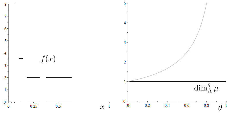
Figure 4: The density $f_{p}$ with $p=1.5$ is plotted on the left and the Assouad spectrum of $\mu_{p}$ is plotted on the right (constant) along with the upper bound from Theorem 2.1 for reference (grey).

4.2 A measure with lower dimension 1 but not in $L^{-1}$.

It is very straightforward to construct a measure with lower dimension equal to 1, but which fails to be in $L^{-1}$. For example, consider the measure with density $f(x)=2x$ on $[0,1]$. For any ball $B(x,r)$ with $0<r<1/2$ we have

$$\mu(B(x,r))=\int_{B(x,r)}f=\int_{\max\{0,x-r\}}^{\min\{1,x+r\}}2ydy=\min\{1,x+r\}^{2}-\max\{0,x-r\}^{2}\approx\begin{cases}r^{2}&x<r\\ xr&r\leqslant x\end{cases}$$

Therefore

$$R/r\lesssim\frac{\mu(B(x,R)}{\mu(B(x,r)}\lesssim(R/r)^{2}$$

with the lower bound attained at $x=1$ and the upper bound attained at $x=0$. This shows $\operatorname{\dim_{\mathrm{L}}}\mu=1<\operatorname{\dim_{\mathrm{A}}}\mu=2$. Further $f\in L^{\infty}([0,1])$ but $f^{-1}(x)=1/x$ and so $f\not\in L^{-1}([0,1])$.

4.2.1 A stronger result for monotonic densities and further work.

Assuming $\mu$ has a monotonic density we can get an implication that is dual to our main theorem (letting $\theta\to 0$).

Proposition 4.2.

Suppose $\mu$ is absolutely continuous with monotonic density $f$ supported on $[0,1]$. If $\operatorname{\dim_{\mathrm{L}}}\mu\geqslant 1-1/p$ for some $p>1$, then $f\in L^{p^{\prime}}([0,1])$ for $1\leqslant p^{\prime}<p$.

Proof.

Without loss of generality we may assume that $f(x)>0$ on $(0,1)$ and non-increasing. Let $0<s<1-1/p<1$, $x=0$ and $0<r<R=1$. Then,

$$C\left(\frac{1}{r}\right)^{s}\leqslant\frac{\int_{B(x,R)}f(x)dx}{\int_{B(x,r)}f(x)dx}=\frac{\int_{0}^{1}f(x)dx}{\int_{0}^{r}f(x)dx}=\frac{1}{\int_{0}^{r}f(x)dx}$$

and so $F(y)=\int_{0}^{y}f(x)dx\leqslant C^{-1}y^{s}$ and, since $f$ is non-increasing, $f(y)\lesssim y^{s-1}$. Therefore

$$\|f\|_{p^{\prime}}\lesssim\int_{0}^{1}x^{p^{\prime}(s-1)}dx<\infty$$

provided $p^{\prime}(1-s)<1$ and therefore $f\in L^{p^{\prime}}([0,1])$ for $p^{\prime}<p$. ∎

It is easily seen that this cannot hold for arbitrary measures. The balanced Bernoulli measure on the Cantor middle third set has lower dimension $\log 2/\log 3$ but is not even absolutely continuous. We do not know if such a result can be proved for absolutely continuous measures.

Question 4.3.

If $\mu\in L^{1}$ and $\operatorname{\dim_{\mathrm{L}}}\mu>0$, then is it true that $\mu\in L^{p}$ for some $p>1$ depending on $\operatorname{\dim_{\mathrm{L}}}\mu$?

One might conjecture the following.

Conjecture 4.4.

If $\mu\in L^{1}$ and $\operatorname{\dim_{\mathrm{L}}}\mu>1-1/p$, then $\mu\in L^{p}$ for $1\leqslant p^{\prime}<p$.

A proof of this conjecture would require finer detail on the implications of measure decay than we were able to establish. Consider, for instance, the following straightforward lemma.

Lemma 4.5.

Let $\mu$ be an absolutely continuous probability measure supported on $[0,1]$ with density $f$. Assume that there exists $C>0$ and $p>1$ such that for all $0<r<R<1$ and $x$ in the support of $\mu$,

$$\frac{\mu(B(x,R))}{\mu(B(x,r))}\geqslant C\left(\frac{R}{r}\right)^{1-1/p}.$$ (4.1)

Let $I_{1}$ and $I_{2}$ be two disjoint intervals of lengths $l_{1}$ and $l_{2}$, respectively, that are separated by an interval of length $d>0$. Then

$$\mu(B(x_{0},R))\geqslant C^{2}\left(\frac{2R}{l_{1}+l_{2}}\right)^{1-1/p}\mu(I_{1}\cup I_{2})$$ (4.2)

for $2R\geqslant l_{1}+l_{2}+2d$ and $x_{0}=a-l_{1}/(l_{1}+l_{2})+d+(l_{1}+l_{2})/2$, where $a$ is the left-hand endpoint of the leftmost of the intervals.

Proof.

Let $x_{1}$ and $x_{2}$ be the midpoints of $I_{1}$ and $I_{2}$, respectively. Without loss of generality we assume $x_{1}<x_{2}$. Let $B_{1}=B(x_{1},l_{1}+d\,l_{1}/(l_{1}+l_{2}))$ and $B_{2}=B(x_{2},l_{2}+dl_{2}/(l_{1}+l_{2}))$ and note that $B_{1}\cap B_{2}=\varnothing$ and $\operatorname{cl}(B_{1})\cup\operatorname{cl}(B_{2})$ is a closed interval containing $I_{1}$ and $I_{2}$ with midpoint $x_{0}$. Here $\operatorname{cl}(\cdot)$ denotes the closure.

Using (4.1), we see that

$$\mu(B_{1}\cup B_{2}) =C\left(\frac{l_{1}+2d\frac{l_{1}}{l_{1}+l_{2}}}{l_{1}}\right)^{1-1/p}\mu(I_{1})+C\left(\frac{l_{2}+2d\frac{l_{2}}{l_{1}+l_{2}}}{l_{2}}\right)^{1-1/p}\mu(I_{2})$$

$$=C\left(1+2d\frac{1}{l_{1}+l_{2}}\right)^{1-1/p}(\mu(I_{1})+\mu(I_{2}))$$

$$=C\left(\frac{l_{1}+l_{2}+2d}{l_{1}+l_{2}}\right)^{1-1/p}\mu(I_{1}\cup I_{2}).$$

Using (4.1) once more for $2R>l_{1}+l_{2}+2d$ we obtain

$$\mu(B(x_{0},R))\geqslant C\left(\frac{2R}{l_{1}+l_{2}+2d}\right)^{1-1/p}\mu(B_{1}\cup B_{2})=C^{2}\left(\frac{2R}{l_{1}+l_{2}}\right)^{1-1/p}\mu(I_{1}\cup I_{2})$$

as required. ∎

Observe that (4.2) resembles the formula one obtains for an interval $I_{0}$ of length $l_{1}+l_{2}$ centred at $x_{0}$ with mass $\mu(I_{1}\cup I_{2})$, namely

$$\mu(B(x_{0},R))\geqslant C\left(\frac{2R}{l_{1}+l_{2}}\right)^{1-1/p}\mu(I_{1}\cup I_{2}),$$

albeit with an additional factor of $C$. This suggests that this scheme can be iterated, though the additional constant $C$ as well as the restriction $R>l_{1}+l_{2}+2d$ do not allow this directly. While we were unable to show this, we suspect that such an iteration can be used to show a statement such as

Conjecture 4.6.

Let $\mu$ and $f$ be as in Lemma 4.5 with the additional assumption that $C\geqslant 1$. Let $\{I_{i}\}$ be a finite set of pairwise disjoint intervals with $\mu(I_{i})\geqslant\varrho\lambda(I_{i})$, where $\lambda$ denotes Lebesgue measure. Then,

$$\varrho^{\,p}\lesssim\frac{1}{\sum_{i=1}^{N}\lambda(I_{i})}.$$

A special case occurs if all $N$ intervals are of equal length $l$ and equally spaced. Let $x_{i}$ be the midpoint of $I_{i}$. Then

$$1=\mu(B(\tfrac{1}{2},\tfrac{1}{2}))=\sum_{i=1}^{N}\mu(B(x_{i}))\geqslant\sum_{i=1}^{N}C\left(\frac{1/N}{l}\right)^{1-1/p}\mu(I_{i})\geqslant N\varrho\,l\left(\frac{1}{Nl}\right)^{1-1/p}=\varrho\,(N\,l)^{1/p}$$

and so $\varrho^{p}\leqslant(N\,l)^{-1}$ as required.

We can also imagine why this might not hold if $C<1$. Suppose $C<1$ and place $2^{n}$ intervals of length $l$ in a “Cantor-like” arrangement, where pairs are separated by a gap of size $\alpha$, pairs of pairs are separated by $\alpha^{2}$, and so on. Then $\alpha>1$ can be picked such that $C(\alpha l/l)^{1-1/p}=1$, implying that $f(x)=0$ and the lower dimension condition is still satisfied.

However, equipped with a statement like Conjecture 4.5 one can prove Conjecture 4.4.

Proof of Conjecture 4.4 using Conjecture 4.6.

Let $\operatorname{\mathfrak{L}}$ be the Lebesgue points of $f(x)$, i.e. the set of points $x$ where $0\leqslant f(x)<\infty$ and

$$g_{k}(x)=\frac{1}{2}\int_{B(x,2^{-k})}2^{k}|f(y)-f(x)|d\lambda(y)\to 0\qquad\text{as}\;k\to\infty.$$

Define $A_{0}=\{x\in\operatorname{\mathfrak{L}}\;:\;f(x)<1\}$ and $A_{k}=\{x\in\operatorname{\mathfrak{L}}\;:\;2^{k}\leqslant f(x)<2^{k+1}\}$ for $k\in\operatorname{\mathbb{N}}$. Note that $\lambda(\operatorname{\mathfrak{L}})=1$ and $\|f\|_{p}^{p}=\int_{[0,1]}f^{p}d\lambda=\sum_{i=0}^{\infty}\int_{A_{k}}f^{p}d\lambda$ where $\lambda$ is Lebesgue measure.

Fix $\operatorname{\varepsilon}>0$ and temporarily fix $k\in\operatorname{\mathbb{N}}_{0}$. We first show that $\int_{A_{k}}f^{p-\operatorname{\varepsilon}}d\lambda\lesssim 2^{-\operatorname{\varepsilon}k}$. If $\mu(A_{k})=0$ we are done. For $k=0$, we get the bound $\int_{A_{0}}f^{p-\operatorname{\varepsilon}}d\lambda\leqslant 1$. Hence we can assume $k\geqslant 1$ and $\mu(A_{k})\neq 0$. Let $0<\delta<\min\{2^{-pk},\mu(A_{k})\}$. Then, by Egoroff’s theorem, there exists $B_{\delta}\subseteq\operatorname{\mathfrak{L}}$ with $\lambda(B_{\delta})>1-\delta$ such that $g_{k}(x)\to 0$ uniformly over $x\in B_{\delta}$. Let $l$ be large enough such that $2^{-l}<\operatorname{\varepsilon}$ and $g_{l^{\prime}}(x)<\operatorname{\varepsilon}$ for all $l^{\prime}\geqslant l$ and $x\in B_{\delta}$. Now let $I=\bigcup_{x\in B_{\delta}\cap A_{k}}B(x,2^{-l})$ and note that $I$ is a finite collection of intervals $\{I_{i}\}$ with $\lambda(I_{i})\geqslant 2^{-l}$. We obtain

$$\int_{I}f^{p-\operatorname{\varepsilon}}d\lambda\leqslant\sum_{i=1}^{\#\{I_{i}\}}\lambda(I_{i})\left(2^{k+1}+\delta\right)^{p-\operatorname{\varepsilon}}\leqslant\sum_{i=1}^{\#\{I_{i}\}}\lambda(I_{i})2^{(k+2)(p-\operatorname{\varepsilon})}.$$

and so, using Conjecture 4.6,

$$\int_{A_{k}}f^{p-\operatorname{\varepsilon}}d\lambda\leqslant\int_{A_{k}\cap B_{\delta}}f^{p-\delta}d\lambda+\int_{A_{k}\cap([0,1]\setminus B_{\delta})}f^{p-\operatorname{\varepsilon}}d\lambda\leqslant 2^{2(p-\operatorname{\varepsilon})}2^{k(p-\operatorname{\varepsilon})}\sum_{i=1}^{\#\{I_{i}\}}\lambda(I_{i})\;+\;\lambda([0,1]\setminus B_{\delta})2^{(p-\operatorname{\varepsilon})k}\lesssim 2^{-\operatorname{\varepsilon}k}.$$

Finally,

$$\|f\|^{p-\operatorname{\varepsilon}}_{p-\operatorname{\varepsilon}}d\lambda=\sum_{k=0}^{\infty}\int_{A_{k}}f^{p-\operatorname{\varepsilon}}d\lambda\leqslant\sum_{k=0}^{\infty}2^{-\operatorname{\varepsilon}k}<\infty$$

and so $\mu\in L^{p-\operatorname{\varepsilon}}$ and letting $\operatorname{\varepsilon}\to 0$ proves Conjecture 4.4. ∎

5 Absolute continuity with general reference measures.

For completeness we include the following result which considers absolute continuity with respect to general reference measures, the proof of which is almost identical to Theorem 2.1

Theorem 5.1.

Let $\nu$ be a measure supported on a non-empty compact set $X\subseteq\operatorname{\mathbb{R}}^{d}$ and suppose $s,t\geqslant 0$ are such that for all $x\in X$ and $r>0$

$$r^{s}\lesssim\mu(B(x,r))\lesssim r^{t}.$$ (5.1)

Suppose $\mu$ is a measure that is absolutely continuous with respect to $\nu$ and suppose $p_{1},p_{2}\in[1,\infty)$ are such that

$$\lVert f\rVert_{p_{1}}=\int_{X}f^{p_{1}}d\nu<\infty\quad\text{and}\quad\lVert f\rVert_{-p_{2}}=\int_{X}f^{-p_{2}}d\nu<\infty.$$

Then

$$\operatorname{{\dim}_{\mathrm{A}}^{\theta}}\mu\leqslant\frac{s-\theta t}{1-\theta}+\frac{p_{1}s+\theta p_{2}t}{p_{1}p_{2}(1-\theta)}\quad\text{and}\quad\operatorname{{\dim}_{\mathrm{L}}^{\theta}}\mu\geqslant\frac{t-\theta s}{1-\theta}-\frac{\theta p_{1}s+p_{2}t}{p_{1}p_{2}(1-\theta)}.$$

Proof.

Fix $\theta\in(0,1)$ and $0<r=R^{1/\theta}\leqslant 1$. Write $q_{1}\in(1,\infty)$ for the Hölder conjugate of $p_{1}$. Then, by Hölder’s inequality

$$\frac{\mu(B(x,R))}{\mu(B(x,r))}\leqslant\frac{\lVert f\rVert_{p_{1}}\lVert\chi_{B(x,R)}\rVert_{q_{1}}}{\lVert f\rVert_{-p_{2}}\lVert\chi_{B(x,r)}\rVert_{p_{2}/(1+p_{2})}} \lesssim\frac{\left(\int\chi_{B(x,R)}^{q_{1}}d\nu\right)^{1/q_{1}}}{\left(\int\chi_{B(x,r)}^{p_{2}/(1+p_{2})}d\nu\right)^{1+1/p_{2}}}$$

$$\lesssim\dfrac{R^{t(1-1/p_{1})}}{r^{s(1+1/p_{2})}}\quad\text{(by \eqref{regdi})}$$

$$=\left(\frac{R}{r}\right)^{\frac{t(1-1/p_{1})-s(1+1/p_{2})/\theta}{1-1/\theta}}.$$

Therefore,

$$\operatorname{{\dim}_{\mathrm{A}}^{\theta}}\mu\leqslant\frac{t(1-1/p_{1})-s(1+1/p_{2})/\theta}{1-1/\theta}=\frac{s-\theta t}{1-\theta}+\frac{p_{1}s+\theta p_{2}t}{p_{1}p_{2}(1-\theta)},$$

as required. The estimate for the lower spectrum is similar and omitted, see the proof of Theorem 2.1. ∎

Note that, for all $\varepsilon>0$, we can always choose $s$ and $t$ in the statement of Theorem 5.1 satisfying

$$\operatorname{\dim_{\mathrm{L}}}\nu-\varepsilon\leqslant t\leqslant s\leqslant\operatorname{\dim_{\mathrm{A}}}\mu+\varepsilon$$

but better choices are sometimes possible.

References

- [F19] J. M. Fraser. Interpolating between dimensions, Proceedings of Fractal Geometry and Stochastics VI, Birkhäuser, Progress in Probability, 2019, (to appear). Preprint available at arXiv:1905.11274.
- [FHHTY18] J. M. Fraser, K. E. Hare, K. G. Hare, S. Troscheit and H. Yu. The Assouad spectrum and the quasi-Assouad dimension: a tale of two spectra, Ann. Acad. Sci. Fenn. Math., 44, (2019), 379–387.
- [FH18] J. M. Fraser and D. Howroyd. On the upper regularity dimensions of measures, Indiana Univ. Math. J., (to appear).
- [FY18] J. M. Fraser and H. Yu. New dimension spectra: finer information on scaling and homogeneity, Adv. Math., 329, (2018), 273–328.
- [HHT19] K. E. Hare, K. G. Hare, and S. Troscheit. Quasi-doubling of self-similar measures with overlaps, J. Fractal Geom., (to appear), arXiv:1807.09198.
- [HT18] K. E. Hare and S. Troscheit. Lower Assouad dimension of measures and regularity, Math. Proc. Cambridge Philos. Soc., (to appear).
- [KL17] A. Käenmäki and J. Lehrbäck. Measures with predetermined regularity and inhomogeneous self-similar sets, Ark. Mat., 33, (2017), 165–184.
- [KLV13] A. Käenmäki, J. Lehrbäck, and M. Vuorinen. Dimensions, Whitney covers, and tubular neighbourhoods, Indiana Univ. Math. J., 62, (2013), 1861–1889.
- [LX16] F. Lü and L. Xi. Quasi-Assouad dimension of fractals, J. Fractal Geom., 3, (2016), 187–215.