More Data Can Hurt for Linear Regression:
Sample-wise Double Descent

Abstract

In this expository note we describe a surprising phenomenon in overparameterized linear regression, where the dimension exceeds the number of samples: there is a regime where the test risk of the estimator found by gradient descent increases with additional samples. In other words, more data actually hurts the estimator. This behavior is implicit in a recent line of theoretical works analyzing “double descent” phenomena in linear models. In this note, we isolate and understand this behavior in an extremely simple setting: linear regression with isotropic Gaussian covariates. In particular, this occurs due to an unconventional type of bias-variance tradeoff in the overparameterized regime: the bias decreases with more samples, but variance increases.

1 Introduction

Common statistical intuition suggests that more data should never harm the performance of an estimator. It was recently highlighted in [Nakkiran et al., 2019] that this may not hold for overparameterized models: there are settings in modern deep learning where training on more data actually hurts. In this note, we analyze a simple setting to understand the mechanisms behind this behavior.

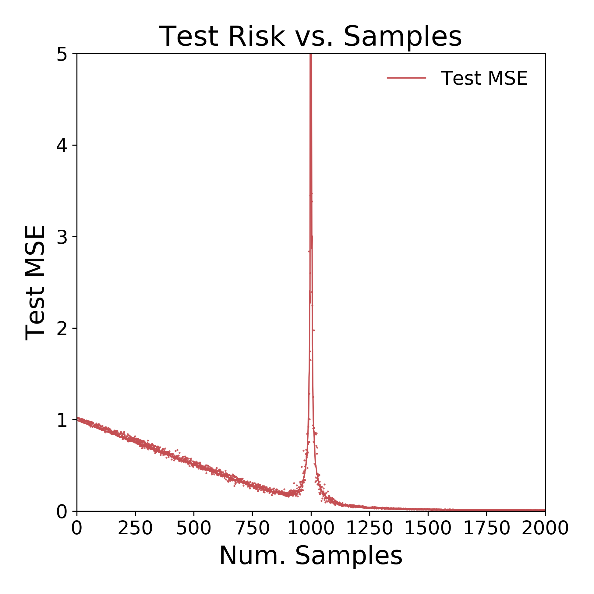
(a) Test MSE for $d=1000,\sigma=0.1$.

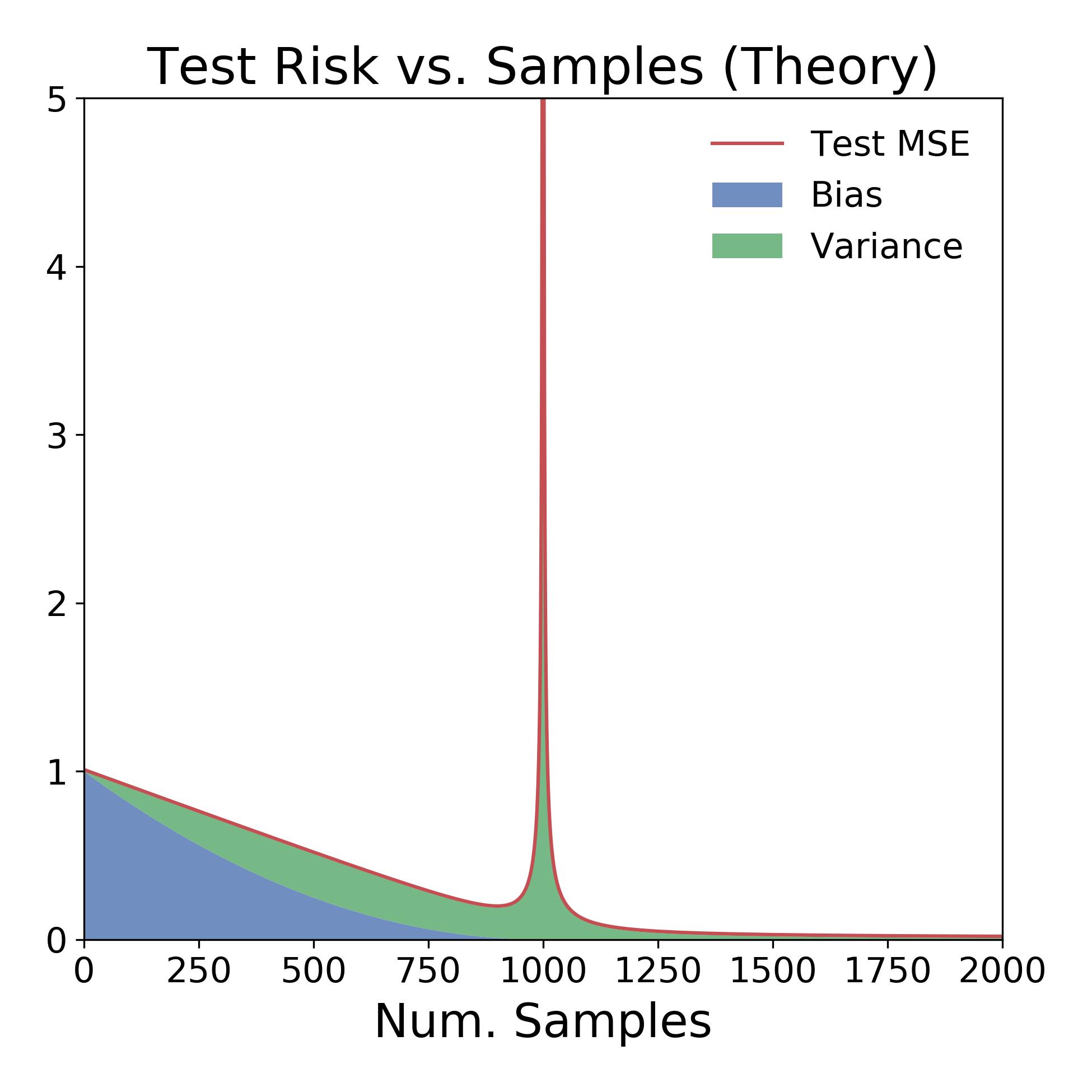
(b) Test MSE in theory for $d=1000,\sigma=0.1$

Figure 1: Test MSE vs. Num. Train Samples for the min-norm ridgeless regression estimator in $d=1000$ dimensions. The distribution is a linear model with noise: covariates $x\sim\mathcal{N}(0,I_{d})$ and response $y=\langle x,\beta\rangle+\mathcal{N}(0,\sigma^{2})$, for $d=1000,\sigma=0.1$, and $||\beta||_{2}=1$. The estimator is $\hat{\beta}=X^{\dagger}y$. Left: Solid line shows mean over 50 trials, and individual points show a single trial. Right: Theoretical predictions for the bias, variance, and risk from Claims 1 and 2.

We focus on well-specified linear regression with Gaussian covariates, and we analyze the test risk of the minimum-norm ridgeless regression estimator— or equivalently, the estimator found by gradient descent on the least squares objective. We show that as we increase the number of samples, performance is non-monotonic: The test risk first decreases, and then increases, before decreasing again.

Such a “double-descent” behavior has been observed in the behavior of test risk as a function of the model size in a variety of machine learning settings [Opper, 1995, Opper, 2001, Advani and Saxe, 2017, Belkin et al., 2018, Spigler et al., 2018, Geiger et al., 2019, Nakkiran et al., 2019]. Many of these works are motivated by understanding the test risk as function of model size, for a fixed number of samples. In this work, we take a complementary view and understand the test risk as a function of sample size, for a fixed model. We hope that understanding such simple settings can eventually lead to understanding the general phenomenon, and lead us to design learning algorithms which make the best use of data (and in particular, are monotonic in samples).

We note that similar analyses appear in recent works, which we discuss in Section 1.1– our focus is to highlight the sample non-monotonicity implicit in these works, and give intuitions for the mechanisms behind it. We specifically refer the reader to [Hastie et al., 2019, Mei and Montanari, 2019] for analysis in a setting most similar to ours.

Organization.

We first define the linear regression setting in Section 2. Then in Section 3 we state the form of the estimator found by gradient descent, and give intuitions for why this estimator has a peak in test risk when the number of samples is equal to the ambient dimension. In Section 3.1, we decompose the expected excess risk into bias and variance contributions, and we state approximate expressions for the bias, variance, and excess risk as a function of samples. We show that these approximate theoretical predictions closely agree with practice, as in Figure 1.

The peak in test risk turns out to be related to the conditioning of the data matrix, and in Section 3.2 we give intuitions for why this matrix is poorly conditioned in the “critical regime”, but well conditioned outside of it. We also analyze the marginal effect of adding a single sample to the test risk, in Section 3.3. We conclude with discussion and open questions in Section 4.

1.1 Related Works

This work was inspired by the long line of work studying “double descent” phenomena in deep and shallow models. The general principle is that as the model complexity increases, the test risk of trained models first decreases and then increases (the standard U-shape), and then decreases again. The peak in test risk occurs in the “critical regime” when the models are just barely able to fit the training set. The second descent occurs in the “overparameterized regime”, when the model capacity is large enough to contain several interpolants on the training data. This phenomenon appears to be fairly universal among natural learning algorithms, and is observed in simple settings such as linear regression, random features regression, classification with random forests, as well as modern neural networks. Double descent of test risk with model size was introduced in generality by [Belkin et al., 2018], building on similar behavior observed as early as [Opper, 1995, Opper, 2001] and more recently by [Advani and Saxe, 2017, Neal et al., 2018, Spigler et al., 2018, Geiger et al., 2019]. A generalized double descent phenomenon was demonstrated on modern deep networks by [Nakkiran et al., 2019], which also highlighted “sample-wise nonmonotonicity” as a consequence of double descent – showing that more data can hurt for deep neural networks.

A number of recent works theoretically analyze the double descent behavior in simplified settings, often for linear models [Belkin et al., 2019, Hastie et al., 2019, Bartlett et al., 2019, Muthukumar et al., 2019, Bibas et al., 2019, Mitra, 2019, Mei and Montanari, 2019, Liang and Rakhlin, 2018, Liang et al., 2019, Xu and Hsu, 2019, Dereziński et al., 2019, Lampinen and Ganguli, 2018, Deng et al., 2019]. At a high level, these works analyze the test risk of estimators in overparameterized linear regression with different assumptions on the covariates. We specifically refer the reader to [Hastie et al., 2019, Mei and Montanari, 2019] for rigorous analysis in a setting most similar to ours. In particular, [Hastie et al., 2019] considers the asymptotic risk of the minimum norm ridgeless regression estimator in the limit where dimension $d$ and number of samples $n$ are scaled as $d\to\infty,n=\gamma d$. We instead focus on the sample-wise perspective: a fixed large $d$, but varying $n$. In terms of technical content, the analysis technique is not novel to our work, and similar calculations appear in some of the prior works above. Our main contribution is highlighting the sample non-monotonic behavior in a simple setting, and elaborating on the mechanisms responsible.

While many of the above theoretical results are qualitatively similar, we highlight one interesting distinction: our setting is well-specified, and the bias of the estimator is monotone nonincreasing in number of samples (see Equation 3, and also [Hastie et al., 2019, Section 3]). In contrast, for misspecified problems (e.g. when the ground-truth is nonlinear, but we learn a linear model), the bias can actually increase with number of samples in addition to the variance increasing (see [Mei and Montanari, 2019]).

2 Problem Setup

Consider the following learning problem: The ground-truth distribution $\mathcal{D}$ is $(x,y)\in\mathbb{R}^{d}\times\mathbb{R}$ with covariates $x\sim\mathcal{N}(0,I_{d})$ and response $y=\langle x,\beta\rangle+\mathcal{N}(0,\sigma^{2})$ for some unknown, arbitrary $\beta$ such that $||\beta||_{2}\leq 1$. That is, the ground-truth is an isotropic Gaussian with observation noise. We are given $n$ samples $(x_{i},y_{i})$ from the distribution, and we want to learn a linear model $f_{\hat{\beta}}(x)=\langle x,\hat{\beta}\rangle$ for estimating $y$ given $x$. That is, we want to find $\hat{\beta}$ with small test mean squared error

$$R(\hat{\beta}) :=\mathop{\mathbb{E}}_{(x,y)\sim\mathcal{D}}[(\langle x,\hat{\beta}\rangle-y)^{2}]$$

$$=||\hat{\beta}-\beta||^{2}+\sigma^{2} x\sim\mathcal{N}(0,I_{d})$$ (for isotropic )

Suppose we do this by performing ridgeless linear regression. Specifically, we run gradient descent initialized at $0$ on the following objective (the empirical risk).

$$\min_{\hat{\beta}}||X\hat{\beta}-y||^{2}$$ (1)

where $X\in\mathbb{R}^{n\times d}$ is the data-matrix of samples $x_{i}$, and $y\in\mathbb{R}^{n}$ are the observations.

The solution found by gradient descent at convergence is $\hat{\beta}=X^{\dagger}y$, where $\dagger$ denotes the Moore–Penrose pseudoinverse. Figure 1(a) plots the expected test MSE of this estimator $\mathop{\mathbb{E}}_{X,y}[R(\hat{\beta}))]$ as we vary the number of train samples $n$. Note that it is non-monotonic, with a peak in test MSE at $n=d$.

There are two surprising aspects of the test risk in Figure 1(a), in the overparameterized regime ($n<d$):

1. The first descent: where test risk initially decreases even when we have less samples $n$ than dimensions $d$. This occurs because the bias decreases.

2. The first ascent: where test risk increases, and peaks when $n=d$. This is because the variance increases, and diverges when $n=d$.

When $n>d$, this is the classical underparameterized regime, and test risk is monotone decreasing with number of samples.

Thus overparameterized linear regression exhibits a bias-variance tradeoff: bias decreases with more samples, but variance can increase. Below, we elaborate on the mechanisms and provide intuition for this non-monotonic behavior.

3 Analysis

The solution found by gradient descent, $\hat{\beta}=X^{\dagger}y$, has different forms depending on the ratio $n/d$. When $n\geq d$, we are in the “underparameterized” regime and there is a unique minimizer of the objective in Equation 1. When $n<d$, we are “overparameterized” and there are many minimizers of Equation 1. In fact, since $X$ is full rank with probability 1, there are many minimizers which interpolate, i.e. $X\hat{\beta}=y$. In this regime, gradient descent finds the minimum with smallest $\ell_{2}$ norm $||\hat{\beta}||^{2}$. That is, the solution can be written as

$$\hat{\beta}=X^{\dagger}y=\begin{dcases}\operatorname*{argmin}_{\begin{subarray}{c}\beta:X\beta=y\end{subarray}}||\beta||^{2}&\text{when $n\leq d$ \quad{\bf(``Overparameterized'')}}\\ \operatorname*{argmin}_{\beta}||X\beta-y||^{2}&\text{when $n>d$ \quad{\bf(``Underparameterized'')}}\end{dcases}$$

The overparameterized form yields insight into why the test MSE peaks at $n=d$. Recall that the observations are noisy, i.e. $y=X\beta+\eta$ where $\eta\sim N(0,\sigma^{2}I_{n})$. When $n\ll d$, there are many interpolating estimators $\{\hat{\beta}:X\hat{\beta}=y\}$, and in particular there exist such $\hat{\beta}$ with small norm. In contrast, when $n=d$, there is exactly one interpolating estimator $(X\hat{\beta}=y)$, but this estimator must have high norm in order to fit the noise $\eta$. More precisely, consider

$$\hat{\beta} =X^{\dagger}y=X^{\dagger}(X\beta+\eta)=\underbrace{X^{\dagger}X\beta}_{\text{signal}}+\underbrace{X^{\dagger}\eta}_{\text{noise}}$$

The signal term $X^{\dagger}X\beta$ is simply the orthogonal projection of $\beta$ onto the rows of $X$. When we are “critically parameterized” and $n\approx d$, the data matrix $X$ is very poorly conditioned, and hence the noise term $X^{\dagger}\eta$ has high norm, overwhelming the signal. This argument is made precise in Section 3.1, and in Section 3.2 we give intuition for why $X$ becomes poorly conditioned when $n\approx d$.

The main point is that when $n=d$, forcing the estimator $\hat{\beta}$ to interpolate the noise will force it to have very high norm, far from the ground-truth $\beta$. (See also Corollary 1 of [Hastie et al., 2019] for a quantification of this point).

3.1 Excess Risk and Bias-Variance Tradeoffs

For ground-truth parameter $\beta$, the excess risk of an estimator $\hat{\beta}$ is:

$$\overline{R}(\hat{\beta}) :=\mathop{\mathbb{E}}_{(x,y)\sim\mathcal{D}}[(\langle x,\hat{\beta}\rangle-y)^{2}]-\mathop{\mathbb{E}}_{(x,y)\sim\mathcal{D}}[(\langle x,\beta\rangle-y)^{2}]$$

$$=\mathop{\mathbb{E}}_{x\sim\mathcal{N}(0,I),\eta\sim\mathcal{N}(0,\sigma^{2})}[(\langle x,\hat{\beta}\rangle-\langle x,\beta\rangle+\eta)^{2}]-\sigma^{2}$$

$$=||\hat{\beta}-\beta||^{2}\$$

For an estimator $\hat{\beta}_{X,y}$ that is derived from samples $(X,y)\sim\mathcal{D}^{n}$, we consider the expected excess risk of $\hat{\beta}=\hat{\beta}_{X,y}$ in expectation over samples $(X,y)$ :

$$\mathop{\mathbb{E}}_{X,y}[\overline{R}(\hat{\beta}_{X,y})]=\mathop{\mathbb{E}}_{X,y}[||\hat{\beta}-\beta||^{2}]=\underbrace{||\beta-\mathop{\mathbb{E}}[\hat{\beta}]||^{2}}_{\text{Bias }B_{n}}+\underbrace{\mathop{\mathbb{E}}[||\hat{\beta}-\mathop{\mathbb{E}}[\hat{\beta}]||^{2}]}_{\text{Variance }V_{n}}$$ (2)

Where $B_{n},V_{n}$ are the bias and variance of the estimator on $n$ samples.

For the specific estimator $\hat{\beta}=X^{\dagger}y$ in the regime $n\leq d$, the bias and variance can be written as (see Appendix A.1):

$$B_{n} =||\mathop{\mathbb{E}}_{X\sim\mathcal{D}^{n}}[\text{Proj}_{X^{\perp}}(\beta)]||^{2}$$ (3)

$$V_{n} =\underbrace{\mathop{\mathbb{E}}_{X}[||\text{Proj}_{X}(\beta)-\mathop{\mathbb{E}}_{X}[\text{Proj}_{X}(\beta)]||^{2}]}_{(A)}+\sigma^{2}\underbrace{\mathop{\mathbb{E}}_{X}[\Tr((XX^{T})^{-1})]}_{(B)}$$ (4)

where $\text{Proj}_{X}$ is the orthogonal projector onto the rowspace of the data $X\in\mathbb{R}^{n\times d}$, and $\text{Proj}_{X^{\perp}}$ is the projector onto the orthogonal complement of the rowspace.

From Equation 3, the bias is non-increasing with samples ($B_{n+1}\leq B_{n}$), since an additional sample can only grow the rowspace: $X_{n+1}^{\perp}\subseteq X_{n}^{\perp}$. The variance in Equation 4 has two terms: the first term (A) is due to the randomness of $X$, and is bounded. But the second term (B) is due to the randomness in the noise of $y$, and diverges when $n\approx d$ since $X$ becomes poorly conditioned. This trace term is responsible for the peak in test MSE at $n=d$.

We can also approximately compute the bias, variance, and excess risk.

Claim 1 (Overparameterized Risk).

Let $\gamma:=\frac{n}{d}<1$ be the underparameterization ratio. The bias and variance are:

$$B_{n} =(1-\gamma)^{2}||\beta||^{2}$$ (5)

$$V_{n} \approx\gamma(1-\gamma)||\beta||^{2}+\sigma^{2}\frac{\gamma}{1-\gamma}$$ (6)

And thus the expected excess risk for $\gamma<1$ is:

$$\mathop{\mathbb{E}}[\overline{R}(\hat{\beta})] \approx(1-\gamma)||\beta||^{2}+\sigma^{2}\frac{\gamma}{1-\gamma}$$ (7)

$$=(1-\frac{n}{d})||\beta||^{2}+\sigma^{2}\frac{n}{d-n}$$ (8)

These approximations are not exact because they hold asyptotically in the limit of large $d$ (when scaling $n=\gamma d$), but may deviate for finite samples. In particular, the bias $B_{n}$ and term (A) of the variance can be computed exactly for finite samples: $\text{Proj}_{X}$ is simply a projector onto a uniformly random $n$-dimensional subspace, so $\mathop{\mathbb{E}}[\text{Proj}_{X}(\beta)]=\gamma\beta$, and similarly $\mathop{\mathbb{E}}[||\text{Proj}_{X}(\beta)||^{2}]=\gamma||\beta||^{2}$. The trace term (B) is nontrivial to understand for finite samples, but converges to $\frac{\gamma}{1-\gamma}$ in the limit of large $n,d$ (e.g. Lemma 3 of [Hastie et al., 2019]). In Section 3.3, we give intuitions for why the trace term converges to this.

For completeness, the bias, variance, and excess risk in the underparameterized regime are given in [Hastie et al., 2019, Theorem 1] as:

Claim 2 (Underparameterized Risk, [Hastie et al., 2019]).

Let $\gamma:=\frac{n}{d}>1$ be the underparameterization ratio. The bias and variance are:

$$B_{n}=0\quad,\quad V_{n}\approx\frac{\sigma^{2}}{\gamma-1}$$

Figure 1 shows that Claims 1 and 2 agree with the excess risk experimentally even for finite $d=1000$.

3.2 Conditioning of the Data Matrix

Here we give intuitions for why the data matrix $X\in\mathbb{R}^{n\times d}$ is well conditioned for $n\ll d$, but has small singular values for $n\approx d$.

3.2.1 Near Criticality

First, let us consider the effect of adding a single sample when $n=(d-1)$. For simplicity, assume the first $(d-1)$ samples $x_{i}$ are just the standard basis vectors, scaled appropriately. That is, assume the data matrix $X\in\mathbb{R}^{(d-1)\times d}$ is

$$X=\matrixquantity[dI_{d-1}&0].$$

This has all non-zero singular values equal to $d$. Then, consider adding a new isotropic Gaussian sample $x_{n+1}\sim\mathcal{N}(0,I_{d})$. Split this into coordinates as $x_{n+1}=(g_{1},g_{2})\in\mathbb{R}^{d-1}\times\mathbb{R}$. The new data matrix is

$$X_{n+1}=\matrixquantity[dI_{d-1}&0\\ g_{1}&g_{2}]$$

We claim that $X_{n+1}$ has small singular values. Indeed, consider left-multiplication by $v^{T}:=\matrixquantity[g_{1}&-d]$:

Thus, $||v^{T}X_{n+1}||^{2}\approx d^{2}$, while $||v||^{2}\approx 2d^{2}$. Since $X_{n+1}$ is full-rank, it must have a singular value less than roughly $\frac{1}{\sqrt{2}}$. That is, adding a new sample has shrunk the minimum non-zero singular value of $X$ from $d$ to less than a constant.

The intuition here is: although the new sample $x_{n+1}$ adds rank to the existing samples, it does so in a very fragile way. Most of the $\ell_{2}$ mass of $x_{n+1}$ is contained in the span of existing samples, and $x_{n}$ only contains a small component outside of this subspace. This causes $X_{n+1}$ to have small singular values, which in turn causes the ridgeless regression estimator (which applies $X^{\dagger}$) to be sensitive to noise.

A more careful analysis shows that the singular values are actually even smaller than the above simplification suggests — since in the real setting, the matrix $X$ was already poorly conditioned even before the new sample $x_{n+1}$. In Section 3.3 we calculate the exact effect of adding a single sample to the excess risk.

3.2.2 Far from Criticality

When $n\ll d$, the data matrix $X$ does not have singular values close to $0$. One way to see this is to notice that since our data model treats features and samples symmetrically, $X$ is well conditioned in the regime $n\ll d$ for the same reason that standard linear regression works in the classical underparameterized regime $n\gg d$ (by “transposing” the setting).

More precisely, since $X$ is full rank, its smallest non-zero singular value can be written as

$$\sigma_{\text{min}}(X)=\min_{v\in\mathbb{R}^{n}:||v||_{2}=1}||v^{T}X||_{2}$$

Since $X$ has entries i.i.d $\mathcal{N}(0,1)$, for every fixed vector $v$ we have $\mathop{\mathbb{E}}_{X}[||v^{T}X||^{2}]=d||v||^{2}=d$. Moreover, for $d=\Omega(n)$ uniform convergence holds, and $||v^{T}X||^{2}$ concentrates around its expectation for all vectors $v$ in the $\ell_{2}$ ball. Thus:

$$\sigma_{\text{min}}(X)^{2}\approx\mathop{\mathbb{E}}_{X}\left[\min_{v\in\mathbb{R}^{n}:||v||_{2}=1}||v^{T}X||^{2}\right]\approx\min_{v}\mathop{\mathbb{E}}_{X}[||v^{T}X||^{2}]=d$$

3.3 Effect of Adding a Single Sample

Here we show how the trace term of the variance in Equation 4 changes with increasing samples. Specifically, the following claim shows how $\Tr((XX^{T})^{-1})$ grows when we add a new sample to $X$.

Claim 3.

Let $X\in\mathbb{R}^{n\times d}$ be the data matrix after $n$ samples, and let $x\in\mathbb{R}^{d}$ be the $(n+1)$th sample. The new data matrix is $X_{n+1}=\matrixquantity[X\\ x^{T}]$, and

$$\Tr((X_{n+1}X_{n+1}^{T})^{-1})=\Tr[(XX^{T})^{-1}]+\frac{1+||(X^{T})^{\dagger}x||^{2}}{||\mathrm{Proj}_{X^{\perp}}(x)||^{2}}$$

Proof.

By computation in Appendix A.2. ∎

If we heuristically assume the denominator concentrates around its expectation, $||\text{Proj}_{X^{\perp}}(x)||^{2}\approx d-n$, then we can use Claim 3 to estimate the expected effect of a single sample:

$$\mathop{\mathbb{E}}_{x}\Tr((X_{n+1}X_{n+1}^{T})^{-1}) \approx\Tr[(XX^{T})^{-1}]+\frac{1+\mathop{\mathbb{E}}_{x}||(XX^{T})^{-1}Xx||^{2}}{d-n}$$ (9)

$$=\Tr[(XX^{T})^{-1}]\left(1+\frac{1}{d-n}\right)+\frac{1}{d-n}$$ (10)

We can further estimate the growth by taking a continuous limit for large $d$. Let $F(\frac{n}{d}):=\mathop{\mathbb{E}}[\Tr((X_{n}X_{n}^{T})^{-1})]$. Then for $\gamma:=\frac{n}{d}$, Equation 10 yields the differential equation

$$\frac{dF(\gamma)}{d\gamma}=(1-\gamma)^{-1}F+(1-\gamma)^{-1}$$

which is solved by $F(\gamma)=\frac{\gamma}{1-\gamma}$. This heuristic derivation that $\mathop{\mathbb{E}}[\Tr(XX^{T})^{-1}]\to\frac{\gamma}{1-\gamma}$ is consistent with the rigorous asymptotics given in [Hastie et al., 2019, Lemma 3] and used in Claim 1.

4 Discussion

We hope that understanding such simple settings can eventually lead to understanding the general behavior of overparameterized models in machine learning. We consider it extremely unsatisfying that the most popular technique in modern machine learning (training an overparameterized neural network with SGD) can be nonmonotonic in samples [Nakkiran et al., 2019]. We hope that a greater understanding here could help develop learning algorithms which make the best use of data (and in particular, are monotonic in samples).

In general, we believe it is interesting to understand when and why learning algorithms are monotonic – especially when we don’t explicitly enforce them to be.

Acknowledgements

We especially thank Jacob Steinhardt and Aditi Raghunathan for discussions and suggestions that motivated this work. We thank Jarosław Błasiok, Jonathan Shi, and Boaz Barak for useful discussions throughout this work, and we thank Gal Kaplun and Benjamin L. Edelman for feedback on an early draft.

This work supported in part by supported by NSF awards CCF 1565264, CNS 1618026, and CCF 1715187, a Simons Investigator Fellowship, and a Simons Investigator Award.

Appendix A Appendix: Computations

A.1 Bias and Variance

The computations in this section are standard.

Assume the data distribution and problem setting from Section 2.

For samples $(X,y)$, the estimator is:

$$\hat{\beta}=X^{\dagger}y=\begin{cases}X^{T}(XX^{T})^{-1}y&\text{when $n\leq d$}\\ (X^{T}X)^{-1}X^{T}y&\text{when $n>d$}\end{cases}$$ (11)

Lemma 1.

For $n\leq d$, the bias and variance of the estimator $\hat{\beta}=X^{\dagger}y$ is

$$B_{n} =||\mathop{\mathbb{E}}_{X\sim\mathcal{D}^{n}}[\text{Proj}_{X^{\perp}}(\beta)]||^{2}$$

$$V_{n} =\underbrace{\mathop{\mathbb{E}}_{X}[||\text{Proj}_{X}(\beta)-\mathop{\mathbb{E}}_{X}[\text{Proj}_{X}(\beta)]||^{2}]}_{(A)}+\sigma^{2}\underbrace{\mathop{\mathbb{E}}_{X}[\Tr((XX^{T})^{-1})]}_{(B)}$$

Proof.

Bias. Note that

$$\beta-\mathop{\mathbb{E}}[\hat{\beta}] =\beta-\mathop{\mathbb{E}}_{X,\eta}[X^{T}(XX^{T})^{-1}(X\beta+\eta)]$$

$$=\mathop{\mathbb{E}}_{X}[(I-X^{T}(XX^{T})^{-1}X)\beta]$$

$$=\mathop{\mathbb{E}}_{X}[Proj_{X^{\perp}}(\beta)]$$

Thus the bias is

$$B_{n} =||\beta-\mathop{\mathbb{E}}[\hat{\beta}]||^{2}$$

$$=||E_{X_{n}}[Proj_{X_{n}^{\perp}}(\beta)]||^{2}$$

Variance.

$$V_{n} =\mathop{\mathbb{E}}_{\hat{\beta}}[||\hat{\beta}-\mathop{\mathbb{E}}[\hat{\beta}]||^{2}]$$

$$=\mathop{\mathbb{E}}_{X,\eta}[||X^{T}(XX^{T})^{-1}(X\beta+\eta)-\mathop{\mathbb{E}}_{X}[X^{T}(XX^{T})^{-1}X\beta]||^{2}]$$

$$=\mathop{\mathbb{E}}_{X,\eta}[||(S-\overline{S})\beta+X^{T}(XX^{T})^{-1}\eta||^{2}] S:=X^{T}(XX^{T})^{-1}X,\overline{S}:=\mathop{\mathbb{E}}[S]$$ ()

$$=\mathop{\mathbb{E}}_{X}[||(S-\overline{S})\beta||^{2}]+\mathop{\mathbb{E}}_{X,\eta}[||X^{T}(XX^{T})^{-1}\eta||^{2}]$$

$$=\mathop{\mathbb{E}}_{X}[||(S-\overline{S})\beta||^{2}]+\sigma^{2}Tr((XX^{T})^{-1})$$

Notice that $S$ is projection onto the rowspace of $X$, i.e. $S=Proj_{X}$. Thus,

$$V_{n}:=\mathop{\mathbb{E}}_{X}[||Proj_{X}(\beta)-\mathop{\mathbb{E}}_{X}[Proj_{X}(\beta)]||^{2}]+\sigma^{2}Tr((XX^{T})^{-1})$$

∎

A.2 Trace Computations

Proof of Claim 3.

Let $X\in\mathbb{R}^{n\times d}$ be the data matrix after $n$ samples, and let $x\in\mathbb{R}^{d}$ be the $(n+1)$th sample. The new data matrix is $X_{n+1}=\matrixquantity[X\\ x^{T}]$, and

$$X_{n+1}X_{n+1}^{T}=\matrixquantity[XX^{T}&Xx\\ x^{T}X^{T}&x^{T}x]$$

Now by Schur complements:

Thus

$$Tr((X_{n+1}X_{n+1}^{T})^{-1}) =Tr((XX^{T}-\frac{Xxx^{T}X^{T}}{||x||^{2}})^{-1})+(||x||^{2}-x^{T}X^{T}(XX^{T})^{-1}Xx)^{-1}$$

$$=Tr((XX^{T}-\frac{Xxx^{T}X^{T}}{||x||^{2}})^{-1})+(x^{T}(x-Proj_{X}(x)))^{-1}$$

$$=Tr((XX^{T}-\frac{Xxx^{T}X^{T}}{||x||^{2}})^{-1})+\frac{1}{||Proj_{X^{\perp}}(x)||^{2}}$$

By Sherman-Morrison:

$$(XX^{T}-\frac{Xxx^{T}X^{T}}{||x||^{2}})^{-1} =(XX^{T})^{-1}+\frac{(XX^{T})^{-1}Xxx^{T}X^{T}(XX^{T})^{-1}}{||x||^{2}-x^{T}X^{T}(XX^{T})^{-1}Xx}$$

$$\implies Tr(XX^{T}-\frac{Xxx^{T}X^{T}}{||x||^{2}})^{-1} =Tr[(XX^{T})^{-1}]+\frac{||(XX^{T})^{-1}Xx||^{2}}{||Proj_{X^{\perp}}(x)||^{2}}$$

Finally, we have

$$Tr((X_{n+1}X_{n+1}^{T})^{-1}) =Tr[(XX^{T})^{-1}]+\frac{1+||(XX^{T})^{-1}Xx||^{2}}{||Proj_{X^{\perp}}(x)||^{2}}$$

or equivalently:

$$Tr((X_{n+1}X_{n+1}^{T})^{-1})=Tr[(XX^{T})^{-1}]+\frac{1+||(X^{T})^{\dagger}x||^{2}}{||Proj_{X^{\perp}}(x)||^{2}}$$

or equivalently:

$$Tr((X_{n+1}X_{n+1}^{T})^{-1})=Tr[(XX^{T})^{-1}]+\frac{1+||\gamma||^{2}}{||Proj_{X^{\perp}}(x)||^{2}}\quad\text{ where }\gamma:=\operatorname*{argmin}_{v}||X^{T}v-x||^{2}$$

∎

References

- [Advani and Saxe, 2017] Advani, M. S. and Saxe, A. M. (2017). High-dimensional dynamics of generalization error in neural networks. arXiv preprint arXiv:1710.03667.
- [Bartlett et al., 2019] Bartlett, P. L., Long, P. M., Lugosi, G., and Tsigler, A. (2019). Benign overfitting in linear regression. arXiv preprint arXiv:1906.11300.
- [Belkin et al., 2018] Belkin, M., Hsu, D., Ma, S., and Mandal, S. (2018). Reconciling modern machine learning and the bias-variance trade-off. arXiv preprint arXiv:1812.11118.
- [Belkin et al., 2019] Belkin, M., Hsu, D., and Xu, J. (2019). Two models of double descent for weak features. arXiv preprint arXiv:1903.07571.
- [Bibas et al., 2019] Bibas, K., Fogel, Y., and Feder, M. (2019). A new look at an old problem: A universal learning approach to linear regression. arXiv preprint arXiv:1905.04708.
- [Deng et al., 2019] Deng, Z., Kammoun, A., and Thrampoulidis, C. (2019). A model of double descent for high-dimensional binary linear classification. arXiv preprint arXiv:1911.05822.
- [Dereziński et al., 2019] Dereziński, M., Liang, F., and Mahoney, M. W. (2019). Exact expressions for double descent and implicit regularization via surrogate random design.
- [Geiger et al., 2019] Geiger, M., Spigler, S., d’Ascoli, S., Sagun, L., Baity-Jesi, M., Biroli, G., and Wyart, M. (2019). Jamming transition as a paradigm to understand the loss landscape of deep neural networks. Physical Review E, 100(1):012115.
- [Hastie et al., 2019] Hastie, T., Montanari, A., Rosset, S., and Tibshirani, R. J. (2019). Surprises in high-dimensional ridgeless least squares interpolation.
- [Lampinen and Ganguli, 2018] Lampinen, A. K. and Ganguli, S. (2018). An analytic theory of generalization dynamics and transfer learning in deep linear networks. arXiv preprint arXiv:1809.10374.
- [Liang and Rakhlin, 2018] Liang, T. and Rakhlin, A. (2018). Just interpolate: Kernel" ridgeless" regression can generalize. arXiv preprint arXiv:1808.00387.
- [Liang et al., 2019] Liang, T., Rakhlin, A., and Zhai, X. (2019). On the risk of minimum-norm interpolants and restricted lower isometry of kernels. arXiv preprint arXiv:1908.10292.
- [Marčenko and Pastur, 1967] Marčenko, V. A. and Pastur, L. A. (1967). Distribution of eigenvalues for some sets of random matrices. Mathematics of the USSR-Sbornik, 1(4):457.
- [Mei and Montanari, 2019] Mei, S. and Montanari, A. (2019). The generalization error of random features regression: Precise asymptotics and double descent curve. arXiv preprint arXiv:1908.05355.
- [Mitra, 2019] Mitra, P. P. (2019). Understanding overfitting peaks in generalization error: Analytical risk curves for l2 and l1 penalized interpolation. ArXiv, abs/1906.03667.
- [Muthukumar et al., 2019] Muthukumar, V., Vodrahalli, K., and Sahai, A. (2019). Harmless interpolation of noisy data in regression. arXiv preprint arXiv:1903.09139.
- [Nakkiran et al., 2019] Nakkiran, P., Kaplun, G., Bansal, Y., Yang, T., Barak, B., and Sutskever, I. (2019). Deep double descent: Where bigger models and more data hurt. arXiv preprint arXiv:1912.02292.
- [Neal et al., 2018] Neal, B., Mittal, S., Baratin, A., Tantia, V., Scicluna, M., Lacoste-Julien, S., and Mitliagkas, I. (2018). A modern take on the bias-variance tradeoff in neural networks. arXiv preprint arXiv:1810.08591.
- [Opper, 1995] Opper, M. (1995). Statistical mechanics of learning: Generalization. The Handbook of Brain Theory and Neural Networks, 922-925.
- [Opper, 2001] Opper, M. (2001). Learning to generalize. Frontiers of Life, 3(part 2), pp.763-775.
- [Spigler et al., 2018] Spigler, S., Geiger, M., d’Ascoli, S., Sagun, L., Biroli, G., and Wyart, M. (2018). A jamming transition from under-to over-parametrization affects loss landscape and generalization. arXiv preprint arXiv:1810.09665.
- [Xu and Hsu, 2019] Xu, J. and Hsu, D. J. (2019). On the number of variables to use in principal component regression. In Advances in Neural Information Processing Systems, pages 5095–5104.