Resonant generation of $p$-wave Cooper pair in non-Hermitian Kitaev chain at exceptional point

Abstract

We investigate a non-Hermitian extension of Kitaev chain by considering imaginary $p$-wave pairing amplitudes. The exact solution shows that the phase diagram consists two phases with real and complex  Bogoliubov-de-gens spectra, associated with $\mathcal{PT}$-symmetry breaking, which is separated by a hyperbolic exceptional line. The exceptional points (EPs) correspond to a specific Cooper pair state $(1+c_{k}^{\dagger}c_{-k}^{\dagger})\left|0\right\rangle$ with movable $k$ when the parameters vary along the exceptional line. The non-Hermiticity around EP supports resonant generation of such a pair state from the vacuum state $\left|0\right\rangle$ of fermions via the critical dynamic process. In addition, we propose a scheme to generate a superconducting state through a dynamic method.

I Introduction

The Kitaev model is a lattice model of a $p$-wave superconducting wire, which realize Majorana zero modes at the ends of the chain Kitaev . This has been demonstrated by unpaired Majorana modes exponentially localized at the ends of open Kitaev chains Sarma ; Stern ; Alicea . The main feature of this model originates from the pairing term, which violates the conservation of the fermion number but preserves its parity, leading to the superconducting phase. The amplitudes for pair creation and annihilation plays an important role in the existence of the gapped superconducting phase. In general, most of the investigations on this model has focused on the case with a Hermitian pairing term. A non-Hermitian term is no longer forbidden both in theory and experiment since the discovery that a certain class of non-Hermitian Hamiltonians could exhibit entirely real spectra Bender ; Bender1 . The origin of the reality of the spectrum of a non-Hermitian Hamiltonian is the pseudo-Hermiticity of the Hamiltonian operator Ali1 . It motives a non-Hermitian extension of the Kitaev model. Many contributions have been devoted to non-Hermitian Kitaev models Law ; Tong ; Yuce ; You ; Klett ; Menke and Ising models ZXZ ; LCPRB within the pseudo-Hermitian framework. Also, the experimental schemes for realizing the Kitaev model and related non-Hermitian systems has been presented in Refs. Franz and Ueda , respectively. In addition, the peculiar features of a non-Hermitian system do not only manifest in statics but also dynamics. From the perspective of non-Hermitian quantum mechanics, it is also a challenge to deal with many-particle dynamics.

In this paper, we investigate a non-Hermitian extension of Kitaev chain by considering imaginary $p$-wave pairing amplitudes. Theoretically, an open system is regarded as a subsystem of an infinite Hermitian system, while a non-Hermitian Hamiltonian is introduced to describe the physics of the subsystem in a phenomenological way Rotter . Non-Hermitian $p$-wave pairing amplitudes may arise from the case, in which subsystem and the surrounding system are in the superconducting phase. When the whole system is in some non-equilibrium superconducting states, the subsystem should be effectively described by a non-Hermitian pair creation and annihilation. As a concrete step toward this, the quantum tunneling of particle pairs has been studied for two weakly interacting systems as a superconducting tunnel junction Matthews . Non-Hermitian systems exhibit many peculiar dynamic behaviors that never occurred in Hermitian systems. One of the remarkable features is the dynamics at exceptional point (EP) HeissEP ; RotterEPJPA ; HXu or spectral singularity (SS) AMprl ; SLHprb ; AAA ; BFS ; ZXZ2 , where the system has a coalescence state. In this work, we focus on the EP-related dynamic behavior for the many-body system.

Based on the exact solution, we find that the exceptional line is a hyperbolic in parameter space, which separates two regions with real and complex Bogoliubov-de-gens spectra, associated with unbroken and broken $\mathcal{PT}$-symmetric phase, respectively. The EPs move in $k$ space when the parameters vary along the exceptional line. In addition, the critical dynamics supports resonant generation of $p$-wave Cooper pair: a specific pair state $c_{k_{\mathrm{c}}}^{\dagger}c_{-k_{\mathrm{c}}}^{\dagger}\left|0\right\rangle$ with selecting opposite momentum $k_{\mathrm{c}}$ can be generated from the vacuum state $\left|0\right\rangle$ of fermions by natural time evolution. The selected $k_{\mathrm{c}}$ ranges over the Brillouin zone, determined by the parameters. The underlying mechanism stems from the critical dynamics around the EP, that projects an initial state on the coalescing state. Our work also exemplifies the dynamic nature of a non-Hermitian interacting many-particle system. As an application, it provides alternative way to generate a superconducting state from an empty state via critical dynamic process rather than cooling down the temperature.

This paper is organized as follows. In Section II, we describe the model Hamiltonian. In Section III, based on the solutions, we present the phase diagram. In Section IV, we study the dynamics in the unbroken-symmetry region, including the time evolution at exceptional line. In Section V, we focus on the critical dynamics for vacuum state as initial state. In Section VI, we propose a scheme to generate a superconducting state. Finally, we give a summary and discussion in Section VII.

II Non-Hermitian Kitaev model

We consider the following fermionic Hamiltonian on a lattice of length $N$

$$\mathcal{H} = \sum\limits_{j=1}^{N}[-Jc_{j}^{{\dagger}}c_{j+1}+\mathrm{H.c.}-i\Delta c_{j}^{{\dagger}}c_{j+1}^{{\dagger}}$$

$$-i\Delta c_{j+1}c_{j}+\mu\left(2n_{j}-1\right)],$$

where $c_{j}^{{\dagger}}$ $(c_{j})$ is a fermionic creation (annihilation) operator on site $j$, $n_{j}=c_{j}^{{\dagger}}c_{j}$, $J$ the tunneling rate, $\mu$ the chemical potential, and $i\Delta$ the strength of the $p$-wave pair creation (annihilation). We define $c_{N+1}=c_{1}$ for periodic boundary condition. The Hamiltonian (II) is known to have a rich phase diagram in its Hermitian version, i.e., $i\Delta\rightarrow\Delta$, which is a spin-polarized $p$-wave superconductor in one dimension. This system is known to have topological phases in which there is a zero energy Majorana mode at each end of a long chain. It is also the fermionized version of the familiar one-dimensional transverse-field Ising model Pfeuty , which is one of the simplest solvable models exhibiting quantum criticality and demonstrating a quantum phase transition with spontaneous symmetry breaking SachdevBook . In this work, we consider a non-Hermitian extension by imaginary pairing amplitude $i\Delta$. Comparing with the non-Hermitian Kitaev model in previous works Law ; Tong ; Yuce ; You ; Klett ; Menke ; LCPRB , the present model has parity-time-reversal ($\mathcal{PT}$) symmetry (proved below) and its non-Hermiticity arises from the imaginary pairing term rather than from the on-site potential term. We will show that the quasi-particle spectrum can have two movable EPs, resulting in some exclusive features different from its Hermitian version.

Before solving the Hamiltonian, it is profitable to investigate the symmetry of the system. By the direct derivation, we have $\left[\mathcal{PT},\mathcal{H}\right]=0$, where the antilinear time reversal operator $\mathcal{T}$ has the function $\mathcal{T}i\mathcal{T=-}i$, and $\left(\mathcal{P}\right)^{-1}c_{l}\mathcal{P}=c_{N-l+1}$. As a usual pseudo-Hermitian system Ali , the $\mathcal{PT}$ symmetry in the present model plays the same role to the phase diagram. The spectrum of $\mathcal{H}$ can be real if all the eigenstates can be written as a $\mathcal{PT}$-symmetric form, while complex when the corresponding eigenstates break the $\mathcal{PT}$-symmetry. The concept of EPs in this paper specifies the locations in the parameter space, at which the complex spectrum starts to appear (In general, an EP is any point with coalescing state). We concentrate our work on the real-spectrum (or unbroken symmetry) region, avoiding the exponentially increased Dirac probability.

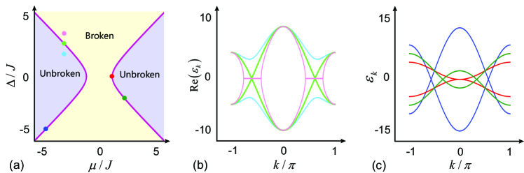
Figure 1: (a) The phase diagram of the non-Hermitian Kitaev model with imaginary p-wave pairing amplitudes. The phase boundary is a hyperbolic exceptional lines (darkmagenta), which separate two regions with real (purple) and complex (yellow) Bogoliubov-de-gens spectra, associated with unbroken $\mathcal{PT}$-symmetric phase and broken $\mathcal{PT}$-symmetric phase respectively. (b) Real part of quasi-particle spectra for three typical points indicated in (a), representing unbroken phase (lightblue), EP line (lightgreen) and broken phase (lightpink), respectively. (c) Quasi-particle spectra for three typical points at the phase boundary line indicated in (a). The corresponding EPs are movable and merges at fixed $k=0$ or $k=\pi$.

In this work, we focus on the dynamics of such a superconducting system, which motivates a more systematic study. Taking the Fourier transformation

$$c_{j}=\frac{1}{\sqrt{N}}\sum\limits_{k}e^{ikj}c_{k},$$ (2)

for the Hamiltonian (II), with wave vector $k\in(-\pi,\pi]$, we have

$$\mathcal{H} = -\sum_{k}[2\left(J\cos k-\mu\right)c_{k}^{{\dagger}}c_{k}$$ (3)

$$+\Delta\sin k(c_{-k}c_{k}+c_{-k}^{{\dagger}}c_{k}^{{\dagger}})+\mu].$$

For the convenience of further analysis, we express the Hamiltonian by using the Nambu representation

$$\mathcal{H} = \sum_{\pi>k>0}\mathcal{H}_{k},$$ (4)

$$\mathcal{H}_{k} = 2\left(\begin{array}[]{cc}c_{k}^{{\dagger}}&c_{-k}\end{array}\right)\left(\begin{array}[]{cc}\mu-J\cos k&\Delta\sin k\\ -\Delta\sin k&J\cos k-\mu\end{array}\right)\left(\begin{array}[]{c}c_{k}\\ c_{-k}^{{\dagger}}\end{array}\right),$$ (10)

where the Hamiltionian $\mathcal{H}_{k}$ in each invariant subspace satisfies the commutation relation

$$\left[\mathcal{H}_{k},\mathcal{H}_{k^{\prime}}\right]=0.$$ (12)

This allows us to treat the diagonalization and the dynamics governed by $\mathcal{H}_{k}$ individually. So far the procedure is the same as those for solving the Hermitian version of $\mathcal{H}$. To diagonalize a non-Hermitian Hamiltonian, we should introduce the Bogoliubov transformation in the complex version:

$$\left\{\begin{array}[]{l}\gamma_{k}=\cos\theta_{k}c_{k}-i\sin\theta_{k}c_{-k}^{{\dagger}},\\ \overline{\gamma}_{k}=\cos\theta_{k}c_{k}^{\dagger}+i\sin\theta_{k}c_{-k},\end{array}\right.$$ (13)

where the complex angle $\theta_{k}$ is determined by

$$\tan\left(2\theta_{k}\right)=\frac{i\Delta\sin k}{\mu-J\cos k}.$$ (14)

It is a crucial step to diagonalize a non-Hermitian Hamiltonian, which essentially establishes the biorthogonal modes. It is easy to check that the complex Bogoliubov modes $\left(\gamma_{k},\overline{\gamma}_{k}\right)$ satisfy the anticommutation relations

$$\left\{\gamma_{k},\overline{\gamma}_{k^{\prime}}\right\} = \delta_{k,k^{\prime}},$$ (15)

$$\left\{\gamma_{k},\gamma_{k^{\prime}}\right\} = \left\{\overline{\gamma}_{k},\overline{\gamma}_{k^{\prime}}\right\}=0,$$

which result in the diagonal form of the Hamiltonian

$$\mathcal{H}=\sum\limits_{k}\varepsilon_{k}\left(\overline{\gamma}_{k}\gamma_{k}-\frac{1}{2}\right).$$ (16)

Here

$$\varepsilon_{k}=2\sqrt{\left(\mu-J\cos k\right)^{2}-\Delta^{2}\sin^{2}k}.$$ (17)

is the dispersion relation of the quasiparticle. Note that the Hamiltonian $\mathcal{H}$ is still non-Hermitian due to the fact that $\overline{\gamma}_{k}\neq\gamma_{k}^{{\dagger}}$. In addition, quasi-spectrum $\varepsilon_{k}$ can be real or imaginary, but not zero since the complex Bogoliubov modes $\left(\gamma_{k},\overline{\gamma}_{k}\right)$ is not well-defined if $\varepsilon_{k}=0$, which will be discussed in next section.

III Phase diagram

According to the theory for a pseudo-Hermitian system Ali , the whole parameter space consists of two kinds of regions, symmetry-unbroken one with a fully real spectrum and symmetry-broken one with a complex spectrum, which originates from the over-threshold imaginary pairing amplitudes. The reason can be seen from the following derivation. For a given $k$, the Hamiltonian $\mathcal{H}_{k}$ in the basis ($\left|0\right\rangle_{k}\left|0\right\rangle_{-k}$, $\left|1\right\rangle_{k}\left|1\right\rangle_{-k}$, $\left|1\right\rangle_{k}\left|0\right\rangle_{-k}$, $\left|0\right\rangle_{k}\left|1\right\rangle_{-k}$) is expressed as $4\times 4$ matrix

$$\mathcal{H}_{k}=2\left(\begin{array}[]{cccc}J\cos k-\mu&-\Delta\sin k&0&0\\ \Delta\sin k&\mu-J\cos k&0&0\\ 0&0&0&0\\ 0&0&0&0\end{array}\right).$$ (18)

The eigenstates $\left|\psi_{k\mathrm{\lambda}}^{\pm}\right\rangle$ ($\mathrm{\lambda}=\mathrm{e,o}$ denotes the even/odd parity of the particle number) are

$$\left|\psi_{k\mathrm{e}}^{\pm}\right\rangle = \frac{1}{\sqrt{\Omega_{\mathrm{nh}}^{\pm}}}\left(\left|0\right\rangle_{k}\left|0\right\rangle_{-k}+\beta_{k}^{\pm}\left|1\right\rangle_{k}\left|1\right\rangle_{-k}\right),$$ (19)

$$\left|\psi_{k\mathrm{o}}^{+}\right\rangle = \left|1\right\rangle_{k}\left|0\right\rangle_{-k},\left|\psi_{k\mathrm{o}}^{-}\right\rangle=\left|0\right\rangle_{k}\left|1\right\rangle_{-k},$$ (20)

where $\Omega_{\mathrm{nh}}^{\pm}=1+\left|\beta_{k}^{\pm}\right|^{2}$ is the normalization coefficient in the context of Dirac inner product with

$$\beta_{k}^{\pm}=\frac{\Delta\sin k}{J\cos k-\mu\pm\varepsilon_{k}/2},$$ (21)

and corresponding energies are

$$\varepsilon_{k\mathrm{e}}^{\pm}=\pm\varepsilon_{k},\varepsilon_{k\mathrm{o}}^{\pm}=0.$$ (22)

We note that

$$\left\{\begin{array}[]{cc}\mathcal{PT}\left|\psi_{k\mathrm{e}}^{\pm}\right\rangle=\left|\psi_{k\mathrm{e}}^{\pm}\right\rangle,&\text{for }\left(\varepsilon_{k}\right)^{2}>0\\ \mathcal{PT}\left|\psi_{k\mathrm{e}}^{\pm}\right\rangle=\left|\psi_{k\mathrm{e}}^{\mp}\right\rangle,&\text{for }\left(\varepsilon_{k}\right)^{2}<0\end{array}\right.,$$ (23)

while

$$\mathcal{PT}\left|\psi_{k\mathrm{o}}^{\pm}\right\rangle=e^{\mp ik}\left|\psi_{k\mathrm{o}}^{\pm}\right\rangle,$$ (24)

for both unbroken and broken $\mathcal{PT}$-symmetric phases, where we used the relation

$$\left(\mathcal{PT}\right)^{-1}c_{k}^{\dagger}\mathcal{PT}=e^{-ik}c_{k}^{\dagger}.$$ (25)

As expected, the symmetry of the eigenstates is associated with the reality of the energy level. An eigenstate of $\mathcal{H}$ is constructed as the form

$$\left|\Psi\right\rangle=\prod_{\pi>k>0}\left|\varphi_{k}^{\lambda}\right\rangle,$$ (26)

where the index $\lambda=1,2,3,4$ labels the eigenstate in each $k$ sector, $\left|\varphi_{k}^{1,2}\right\rangle=\left|\psi_{k\mathrm{e}}^{+.-}\right\rangle$ and $\left|\varphi_{k}^{3,4}\right\rangle=\left|\psi_{k\mathrm{o}}^{+.-}\right\rangle$, with the eigen energy

$$E=\sum_{\pi>k>0}\epsilon_{k}^{\lambda},$$ (27)

with $\epsilon_{k}^{1,2}=\varepsilon_{k\mathrm{e}}^{+,-}$ and $\epsilon_{k}^{3,4}=0$. Therefore, the reality of $\varepsilon_{k}$ determines the reality of the spectrum of $\mathcal{H}$, since a single imaginary $\varepsilon_{k}$ can result in the complex spectrum of $\mathcal{H}$. A quantum phase transition occurs when the complex spectrum appears. Then the phase boundary of $\mathcal{H}$ locates at the touching point of curve $\varepsilon_{k}$ at $k$ axis. The phase boundary (or EP line) in parameter space ($\mu-\Delta$ plane) is determined by the equations JLPRA .

$$\varepsilon_{k_{\mathrm{c}}}=\left[\frac{\partial\varepsilon_{k}}{\partial k}\right]_{k=k_{\mathrm{c}}}=0.$$ (28)

The boundary is obtained as

$$\mu_{\mathrm{c}}^{2}-\Delta_{\mathrm{c}}^{2}=J^{2}$$ (29)

with

$$k_{\mathrm{c}}=\arccos\frac{J}{\mu_{\mathrm{c}}}.$$ (30)

In this situation, $\mathcal{H}_{k_{\mathrm{c}}}$ cannot be expressed as the complex Bogoliubov modes $\left(\gamma_{k_{\mathrm{c}}},\overline{\gamma}_{k_{\mathrm{c}}}\right)$ since the matrix of $\mathcal{H}_{k_{\mathrm{c}}}$ in even particle number sector has a Jordan block form

$$M_{\mathrm{c}}=\frac{-2\Delta_{\mathrm{c}}^{2}}{\mu_{\mathrm{c}}}\left(\begin{array}[]{cc}1&-1\\ 1&-1\end{array}\right),$$ (31)

which hence is no longer diagonalizable. Two eigenvectors of $M_{\mathrm{c}}$ coalesce to a single one $\left(1,1\right)^{\mathrm{T}}$, leading to a set of coalescing eigenstates of $\mathcal{H}$, including the coalescing groundstate. Remarkably, $\mathcal{H}_{k_{\mathrm{c}}}$ governs a peculiar dynamics, which is the focus of this work. The phase diagram on parameter $\mu-\Delta$ plane is plotted in Fig. 1(a). The real part of quasi-particle spectra for several typical points in symmetry-unbroken, broken phase phases, and on EP line are plotted in Fig. 1(b) and (c). It shows that the pair of EPs are movable and meet at a fixed point. Such a gapless phase is different from its Hermitian version, where the band touching point is degenerate point. It will result in different dynamical behavior in the non-Hermitian Kitaev model, especially near the phase boundary.

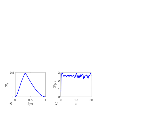
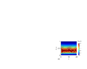
Figure 2: Plots of (a) $\overline{N}_{k}$, (b) ${\overline{N}}(t)$, and (c) $N_{k}(t)$, which is defined in Eqs. (54), (55) and (52). The parameters are $N=40$ and $(J,\Delta,\mu)=(1,\sqrt{3},2)$.

IV Dynamics

We study the dynamics in the unbroken-symmetry region, in which $\varepsilon_{k}$ is always real, including the time evolution at exceptional line. Based on the above analysis, the dynamics is governed by the time evolution operator

$$U(t)=\exp(-i\mathcal{H}t)=\prod_{\pi>k>0}U_{k}(t),$$ (32)

where

$$U_{k}(t)=\exp(-i\mathcal{H}_{k}t).$$ (33)

The explicit form of $U_{k}(t)$ is determined by the diagonal form of $\mathcal{H}_{k}$, i.e.,

$$\mathcal{H}_{k}=\varepsilon_{k}\left(\overline{\gamma}_{k}\gamma_{k}+\overline{\gamma}_{-k}\gamma_{-k}-1\right)$$ (34)

However, one of an exclusive features of a non-Hermitian system is that $\mathcal{H}_{k}$ is undiagonalizable when $k=k_{\mathrm{c}}$. Therefore, we will deal with $U_{k}(t)$ in two aspects.

(i) In the case of $k\neq k_{\mathrm{c}}$, we have

$$U_{k}(t) = 2\left[\cos\left(\varepsilon_{k}t\right)-1\right]\bar{\gamma}_{k}\gamma_{k}\bar{\gamma}_{-k}\gamma_{-k}$$

$$+\left(1-e^{i\varepsilon_{k}t}\right)\left(\bar{\gamma}_{-k}\gamma_{-k}+\bar{\gamma}_{k}\gamma_{k}\right)+e^{i\varepsilon_{k}t},$$

where we have used the identity $\left(\overline{\gamma}_{k}\gamma_{k}\right)^{2}=\overline{\gamma}_{k}\gamma_{k}$. This result is also valid for imaginary $\varepsilon_{k}$. The vacuum state of $\gamma_{k}$ is constructed as $\left|\mathrm{Vac}\right\rangle_{k}=\gamma_{k}\left|0\right\rangle$, where $\left|0\right\rangle$ is the vacuum state of $c_{k}$. Four states ($\left|00\right\rangle_{k}$, $\left|11\right\rangle_{k}$, $\left|10\right\rangle_{k}$, $\left|01\right\rangle_{k}$)=($\left|\mathrm{Vac}\right\rangle_{k}\left|\mathrm{Vac}\right\rangle_{-k}$, $\bar{\gamma}_{k}\bar{\gamma}_{-k}\left|\mathrm{Vac}\right\rangle_{k}\left|\mathrm{Vac}\right\rangle_{-k}$, $\bar{\gamma}_{k}\left|\mathrm{Vac}\right\rangle_{k}\left|\mathrm{Vac}\right\rangle_{-k}$, $\bar{\gamma}_{-k}\left|\mathrm{Vac}\right\rangle_{k}\left|\mathrm{Vac}\right\rangle_{-k}$) are both the eigenstates of $\mathcal{H}_{k}$. The time evolution of such four states are

$$U_{k}(t)\left(\begin{array}[]{c}\left|00\right\rangle_{k}\\ \left|11\right\rangle_{k}\\ \left|10\right\rangle_{k}\\ \left|01\right\rangle_{k}\end{array}\right)=\left(\begin{array}[]{c}\exp\left(i\varepsilon_{k}t\right)\left|00\right\rangle_{k}\\ \exp\left(-i\varepsilon_{k}t\right)\left|11\right\rangle_{k}\\ \left|10\right\rangle_{k}\\ \left|01\right\rangle_{k}\end{array}\right),$$ (36)

which indicates that it looks like the one in Hermitian system if $\varepsilon_{k}$ is real. The corresponding Dirac probability, $\left|U_{k}(t)\left|mn\right\rangle_{k}\right|^{2}$ ($m,n=1,0$) is conservative. However, the Dirac probability of a superposition of such two eigenstates in even particle number subspace is periodic function of time with period $\pi/\varepsilon_{k}$. It is noted that when $k$ tends to $k_{\mathrm{c}}$, this period goes to infinite (or non-period), which is one of properties of the critical dynamics.

(ii) In the case of $k=k_{\mathrm{c}}$, $\mathcal{H}_{k_{\mathrm{c}}}$ cannot be expressed as the complex Bogoliubov modes $\left(\gamma_{k_{\mathrm{c}}},\overline{\gamma}_{k_{\mathrm{c}}}\right)$. Nevertheless, we can rewrite $\mathcal{H}_{k_{\mathrm{c}}}$ in the form

$$\mathcal{H}_{k_{\mathrm{c}}}=-\frac{2\Delta_{\mathrm{c}}^{2}}{\mu_{\mathrm{c}}}\left(s_{k_{\mathrm{c}}}^{z}+is_{k_{\mathrm{c}}}^{y}\right),$$ (37)

by introducing pseudo-spin operators ZGPRL

$$s_{k}^{x} = \frac{1}{2}\left(c_{-k}^{{\dagger}}c_{k}^{{\dagger}}+c_{k}c_{-k}\right),$$

$$s_{k}^{y} = \frac{1}{2i}\left(c_{-k}^{{\dagger}}c_{k}^{{\dagger}}-c_{k}c_{-k}\right),$$

$$s_{k}^{z} = \frac{1}{2}\left(c_{k}^{{\dagger}}c_{k}+c_{-k}^{{\dagger}}c_{-k}-1\right),$$ (38)

which satisfy Lie algebra $[s_{k}^{\alpha},s_{k}^{\beta}]=i\varepsilon_{\alpha\beta\gamma}s_{k}^{\gamma}$, with $\varepsilon_{\alpha\beta\gamma}$ being the Levi-Civita symbol. The corresponding time evolution operator has the form

$$U_{k_{\mathrm{c}}}(t)=\exp(-i\mathcal{H}_{k_{\mathrm{c}}}t)=1-i\mathcal{H}_{k_{\mathrm{c}}}t,$$ (39)

based on the identity $\left(s_{k}^{z}+is_{k}^{y}\right)^{2}=0$, or $\left(\mathcal{H}_{k_{\mathrm{c}}}\right)^{2}=0$.

Obviously, the coalescing eigenstate of $\mathcal{H}_{k_{\mathrm{c}}}$ is the spin-up state in $x$ direction, $s_{k_{\mathrm{c}}}^{x}\left|x\right\rangle=\frac{1}{2}\left|x\right\rangle$, and the corresponding eigenstates are

$$\left|\pm x\right\rangle=\left|0\right\rangle_{k}\left|0\right\rangle_{-k}\pm\left|1\right\rangle_{k}\left|1\right\rangle_{-k}.$$ (40)

Then the dynamics of the Jordan block is very clear, i.e.,

$$U_{k_{\mathrm{c}}}(t)\left|x\right\rangle = \left|x\right\rangle,$$ (41)

$$U_{k_{\mathrm{c}}}(t)\left|-x\right\rangle = \left|-x\right\rangle+i4\left(\Delta_{\mathrm{c}}^{2}/\mu_{\mathrm{c}}\right)t\left|x\right\rangle.$$ (42)

Any initial state with component $\left|x\right\rangle$ obeys a non-periodic (or infinite period) dynamics, which accords with the dynamics of $\mathcal{H}_{k}$ with $k\rightarrow k_{\mathrm{c}}$. In addition, the evolved state $U_{k_{\mathrm{c}}}(t)\left|-x\right\rangle$ converges to $\left|x\right\rangle$ as time increases. This property also appears in the dynamics of $\mathcal{H}_{k}$ with $k\rightarrow k_{\mathrm{c}}$. Therefore, the system around EP should exhibit some peculiar critical dynamics. The dynamics of $\mathcal{H}_{k_{\mathrm{c}}}$ alone cannot induce any macroscopic phenomenon, while a set of $\mathcal{H}_{k}$ near EP may result in many-particle effect.

V P-wave pair generation

In this section, we investigate the critical dynamical behavior by applying the obtained $U(t)$ on a simple initial state. We start with the time evolution of the vacuum state of operators $c_{\pm k}$ as an initial state, i.e.,

$$\left|\psi_{k}(0)\right\rangle=\left|0\right\rangle_{k}\left|0\right\rangle_{-k}.$$ (43)

In the case of $k\neq k_{\mathrm{c}}$, we have

$$\left|\psi_{k}(t)\right\rangle = U_{k}(t)\left|\psi_{k}(0)\right\rangle$$

$$= \left[-2i\sin\left(\varepsilon_{k}t\right)\sin^{2}\theta_{k}+\exp\left(i\varepsilon_{k}t\right)\right]\left|0\right\rangle_{k}\left|0\right\rangle_{-k}$$

$$-\sin\left(2\theta_{k}\right)\sin\left(\varepsilon_{k}t\right)\left|1\right\rangle_{k}\left|1\right\rangle_{-k},$$

while for $k=k_{\mathrm{c}}$, we have

$$\left|\psi_{k_{\mathrm{c}}}(t)\right\rangle=\left(1+it\right)\left|0\right\rangle_{k_{\mathrm{c}}}\left|0\right\rangle_{-k_{\mathrm{c}}}-it\left|1\right\rangle_{k_{\mathrm{c}}}\left|1\right\rangle_{-k_{\mathrm{c}}}.$$ (45)

Accordingly, considering a vacuum state of all fermions (empty state) as an initial state

$$\left|\Psi(0)\right\rangle=\prod_{k>0}\left|\psi_{k}(0)\right\rangle=\prod_{k>0}\left|0\right\rangle_{k}\left|0\right\rangle_{-k},$$ (46)

we have

$$\left|\Psi(t)\right\rangle=\prod_{k>0}U_{k}(t)\left|\psi_{k}(0)\right\rangle.$$ (47)

It is expected $p$-wave pairs are generated from the empty state. We are interested in the normalized population of $p$-wave pair

$$N(t)=\frac{\left\langle\Psi(t)\right|\widehat{N}\left|\Psi(t)\right\rangle}{\left\langle\Psi(t)\right|\Psi(t)\rangle}=\sum_{k>0}\frac{\left\langle\Psi(t)\right|\widehat{N}_{k}\left|\Psi(t)\right\rangle}{\left\langle\Psi(t)\right|\Psi(t)\rangle},$$ (48)

where the total $p$-wave pair number operator is

$$\widehat{N}=\sum_{k>0}\widehat{N}_{k}=\sum_{k>0}n_{k}n_{-k}.$$ (49)

Then $N(t)$ can be evaluated from $N_{k}(t)$

$$N(t)=\sum_{k>0}N_{k}(t)=\sum_{k>0}\frac{\left\langle\psi_{k}(t)\right|\widehat{N}_{k}\left|\psi_{k}(t)\right\rangle}{\left\langle\psi_{k}(t)\right|\psi_{k}(t)\rangle},$$ (50)

and the distribution of $N_{k}(t)$ determines the property of the non-equilibrium state.

For the case of $k\neq k_{\mathrm{c}}$, we have

$$\left\langle\Psi_{k}(t)\right|\Psi_{k}(t)\rangle=2\left|\sin 2\theta_{k}\right|^{2}\sin^{2}\left(\varepsilon_{k}t\right)+1,$$ (51)

and

$$N_{k}(t)=\frac{\left[\Delta\sin k\sin\left(t\varepsilon_{k}\right)\right]^{2}}{\left(\varepsilon_{k}/2\right)^{2}+2\left[\Delta\sin k\sin\left(t\varepsilon_{k}\right)\right]^{2}},$$ (52)

which is a periodic function of time with period $T_{k}=\pi/\varepsilon_{k}$. We note that we have $\varepsilon_{k}\approx 0$ in the vicinity of $k\approx k_{\mathrm{c}}$, and the period become very long. It indicates that we always have $N_{k}(t)\approx 1/2$ except for some short intervals.

For the case of $k=k_{\mathrm{c}}$, Eq. (45) shows that the normalized pair number is

$$N_{k_{\mathrm{c}}}(t)=\frac{t^{2}}{1+2t^{2}},$$ (53)

which obeys lim${}_{t\rightarrow\infty}N_{k_{\mathrm{c}}}(t)=1/2$, which accords with the case with $k\neq k_{\mathrm{c}}$ but infinite long period. In order to demonstrate the property of the evolved state, we define the average normalized pair number distribution

$$\overline{N}_{k}=\frac{1}{T_{k}}\int_{0}^{T_{k}}N_{k}(t)\mathrm{d}t,$$ (54)

and the total average normalized pair number

$$\overline{N}\left(t\right)=\frac{1}{\pi}\int_{0}^{\pi}N_{k}(t)\mathrm{d}k.$$ (55)

We plot quantities $\overline{N}_{k}$, $\overline{N}(t)$, and $N_{k}(t)$ for a concrete cases in Fig. 2. It indicates that the majority of modes become quasi stable after a period of time. Accordingly, the evolved many-body state $\left|\Psi(t)\right\rangle$ should exhibit as a macroscopic equilibrium state. In the following section, we will investigate the possible property of such a state.

VI Dynamical generation of superconducting state

In this section, as an application of above result, we investigate the possibility of dynamical generation of superconducting state via a non-Hermitian Kitaev model. The scheme is that taking the empty state $\sum_{k>0}\left|0\right\rangle_{k}\left|0\right\rangle_{-k}$ as an initial state, the final state, which approches to the ground state of a Hermitian Kitaev Hamiltonian $H$, is acheived by a driven non-Hermitian Kitaev Hamiltonian $\mathcal{H}$ at EP. Before proceeding, we briefly review the properties of a Hermitian Kitaev model with the Hamiltonian

$$H = \sum\limits_{j=1}^{N}[-Jc_{j}^{{\dagger}}c_{j+1}+\mathrm{H.c.}-i\Delta_{\mathrm{h}}c_{j}^{{\dagger}}c_{j+1}^{{\dagger}}$$

$$+i\Delta_{\mathrm{h}}c_{j+1}c_{j}+\mu_{\mathrm{h}}\left(2n_{j}-1\right)].$$

It has been shown to have topologically non-trivial (trivial) ground state, when $\left|\mu_{\mathrm{h}}\right|<\left|J\right|$ ($\left|\mu_{\mathrm{h}}\right|>\left|J\right|$) in Ref. Kitaev . The phase diagram is plotted in Fig. 3, with H-shape boundary separating topologically non-trivial and trivial phases, characterized by winding number $\mathcal{N}$. By the similar procedure as above, we have

$$H = \sum_{\pi>k>0}H_{k},$$ (57)

$$H_{k} = 2\left(\begin{array}[]{cc}c_{k}^{{\dagger}}&c_{-k}\end{array}\right)\left(\begin{array}[]{cc}\mu_{\mathrm{h}}-J\cos k&\Delta_{\mathrm{h}}\sin k\\ \Delta_{\mathrm{h}}\sin k&J\cos k-\mu_{\mathrm{h}}\end{array}\right)\left(\begin{array}[]{c}c_{k}\\ c_{-k}^{{\dagger}}\end{array}\right),$$ (63)

where the Hamiltonian $H_{k}$ in each invariant subspace satisfies the commutation relation

$$\left[H_{k},H_{k^{\prime}}\right]=0.$$ (65)

For a given $k$, the Hamiltonian $H_{k}$ in the basis ($\left|0\right\rangle_{k}\left|0\right\rangle_{-k}$, $\left|1\right\rangle_{k}\left|1\right\rangle_{-k}$, $\left|1\right\rangle_{k}\left|0\right\rangle_{-k}$, $\left|0\right\rangle_{k}\left|1\right\rangle_{-k}$) is expressed as $4\times 4$ matrix

$$h_{k}=2\left(\begin{array}[]{cccc}J\cos k-\mu_{\mathrm{h}}&\Delta_{\mathrm{h}}\sin k&0&0\\ \Delta_{\mathrm{h}}\sin k&\mu_{\mathrm{h}}-J\cos k&0&0\\ 0&0&0&0\\ 0&0&0&0\end{array}\right).$$ (66)

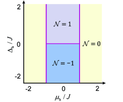
Figure 3: Phase diagram of Hermitian Kitaev model on the parameter $\mu_{h}-\Delta_{h}$ plane. The skyblue, yellow and purple regions correspond to the winding number $-1$, $0$ and $1$ respectively. Darkmagenta lines indicate the phase transition lines.

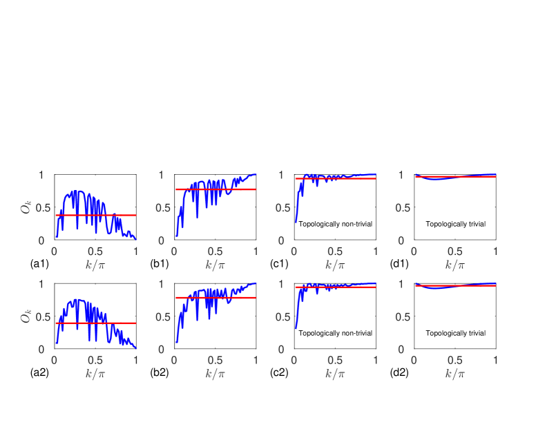
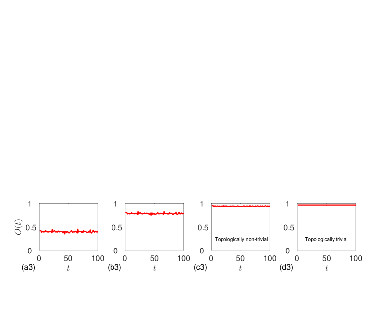
Figure 4: Numerical simulations of $O_{k}$ defined in Eq. (75), and $O\left(t\right)$ defined in Eq. (74). The four panels in first row and the second row are the plots of $O_{k}$ at time $t=50J^{-1}$ and $100J^{-1}$, respectively. The red lines represent the corresponding $O$, which are the values (a1) $0.376$, (a2) $0.390$, (b1) $0.771$, (b2) $0.780$, (c1) $0.936$, (c2) $0.939$, (d1) $0.964$, (d2) $0.964$. The four panels in third row are the plots of $O(t)$ with the same parameters in two above rows. The parameters are $N=61$, $J=1$, $\Delta=\Delta_{\mathrm{h}}=1$, and $\mu=\sqrt{J^{2}+\Delta^{2}}$. Each column of the graph has the same set of parameters, i.e., (a1-a3) $\mu_{\mathrm{h}}=-5$, (b1-b3) $\mu_{\mathrm{h}}=-0.5$, and (c1-c3) $\mu_{\mathrm{h}}=0.9$, (d1-d3) $\mu_{\mathrm{h}}=\mu$. The parameters of Hermitian Kitaev model in (c1-c3) and (d1-d3) supports topologically non-trivial and trivial superconducting ground states, respectively.

The eigenstates $\left|\varphi_{k\mathrm{\lambda}}^{\pm}\right\rangle$ ($\mathrm{\lambda}=\mathrm{e,o}$ denotes the even/odd parity of the particle number) are

$$\left|\varphi_{k\mathrm{e}}^{\pm}\right\rangle = \frac{1}{\sqrt{\Omega_{\mathrm{h}}^{\pm}}}\left(\left|0\right\rangle_{k}\left|0\right\rangle_{-k}+b_{k}^{\pm}\left|1\right\rangle_{k}\left|1\right\rangle_{-k}\right),$$ (67)

$$\left|\varphi_{k\mathrm{o}}^{+}\right\rangle = \left|1\right\rangle_{k}\left|0\right\rangle_{-k},\left|\varphi_{k\mathrm{o}}^{-}\right\rangle=\left|0\right\rangle_{k}\left|1\right\rangle_{-k},$$ (68)

where $\Omega_{\mathrm{h}}^{\pm}=1+\left|b_{k}^{\pm}\right|^{2}$ is the normalization coefficient in the context of Dirac inner product with

$$b_{k}^{\pm}=\frac{\Delta_{\mathrm{h}}\sin k}{J\cos k-\mu_{\mathrm{h}}\pm\epsilon_{k\mathrm{e}}^{\pm}/2},$$ (69)

and corresponding energies are

$$\left\{\begin{array}[]{c}\epsilon_{k\mathrm{e}}^{\pm}=\pm 2\sqrt{\left(\mu_{\mathrm{h}}-J\cos k\right)^{2}+\Delta_{\mathrm{h}}^{2}\sin^{2}k},\\ \epsilon_{k\mathrm{o}}^{\pm}=0.\end{array}\right.$$ (70)

Accordingly, the groundstate wave function can be expressed as

$$\left|\text{{G}}\right\rangle=\prod_{\pi>k>0}\left|\varphi_{k\mathrm{e}}^{-}\right\rangle.$$ (71)

We note that for a topological non-trivial ground state, we have

$$\lim_{k\rightarrow 0}\left|\varphi_{k\mathrm{e}}^{-}\right\rangle=\left|1\right\rangle_{k}\left|1\right\rangle_{-k},\lim_{k\rightarrow\pi}\left|\varphi_{k\mathrm{e}}^{-}\right\rangle=\left|0\right\rangle_{k}\left|0\right\rangle_{-k},$$ (72)

while

$$\lim_{k\rightarrow 0}\left|\varphi_{k\mathrm{e}}^{-}\right\rangle=\left|0\right\rangle_{k}\left|0\right\rangle_{-k},\lim_{k\rightarrow\pi}\left|\varphi_{k\mathrm{e}}^{-}\right\rangle=\left|0\right\rangle_{k}\left|0\right\rangle_{-k},$$ (73)

for a topological trivial ground state. On the other hand, for the non-Hermitian system, we know that there is a stable final state $\lim_{t\rightarrow\infty}\left|\psi_{k_{\mathrm{c}}}(t)\right\rangle\propto(\left|0\right\rangle_{k_{\mathrm{c}}}\left|0\right\rangle_{-k_{\mathrm{c}}}-\left|1\right\rangle_{k_{\mathrm{c}}}\left|1\right\rangle_{-k_{\mathrm{c}}})$, according to Eq. (45). If we take a matching set of parameters, the stable final state can be an eigenmode of $\left|\text{{G}}\right\rangle$ , i.e., $\left|\psi_{k_{\mathrm{c}}}(t)\right\rangle=\left|\varphi_{k_{\mathrm{c}}\mathrm{e}}^{-}\right\rangle$ after normalization. It is probably to obtain a state dynamically under the Hamiltonian $\mathcal{H}$, which is similar to a ground state of $H$. To characterize how close of an evolved state to a superconducting state we introduce a quantity

$$O(t)=\frac{1}{N}\sum_{k}O_{k}(t),$$ (74)

where

$$O_{k}(t)=\left\langle\varphi_{k\mathrm{e}}^{-}\right.\left|\psi_{k}(t)\right\rangle,$$ (75)

is the overlap of a specific topological superconducting mode $\left|\psi_{k\mathrm{e}}^{-}\right\rangle$ and a dynamically generated state $\left|\psi_{k}(t)\right\rangle$ via the non-Hermitian system.

We compute the quantity $O(t)$ for various sets of parameters $\left(J,\Delta,\mu\right)$ and $\left(J,\Delta_{\mathrm{h}},\mu_{\mathrm{h}}\right)$ to search optimal cases with large $O(t)$. We find that there are many cases with large $O(t)$. Here we take four typical cases to demonstrate our results. We plot $O(t)$ and $O_{k}$ at certain instants in Fig. 4, which show that $O(t)$ oscillates with a very small amplitude. It also indicates that through such a dynamical method, a quasi-superconducting state involving topological trivial and non-trivial can be generated from a simple initial state.

VII Summary

In summary, we have studied the non-Hermitian extension of Kitaev chain by considering imaginary $p$-wave pairing amplitudes. Based on the analysis of the exact solution we find that exceptional line is hyperbolic, which separates two regions with real and complex Bogoliubov-de-gens spectra, associated with $\mathcal{PT}$-symmetry breaking. The EPs are movable in $k$ space as the parameters vary along the exceptional line. The non-Hermiticity around EP supports resonant generation of $p$-wave Cooper pair state via the critical dynamic process. A specific pair state $(1+c_{k}^{\dagger}c_{-k}^{\dagger})\left|0\right\rangle$ with selecting momentum $k$ can be generated from the vacuum state $\left|0\right\rangle$ of fermions and be frozen forever. The remarkable result obtained by analytical approaches and numerical simulations are that the dynamically generated state via the non-Hermitian system is very close to a specific superconducting ground state, which can be topologically non-trivial or not. This finding provides alternative way to generate a superconducting state via critical dynamic process rather than cooling down the temperature.

References

- (1) A. Y. Kitaev, Unpaired Majorana fermions in quantum wires, Phys. Usp. 44, 131 (2001).
- (2) C. Nayak, S. H. Simon, A. Stern, M. Freedman, and S. D. Sarma, Non-Abelian anyons and topological quantum computation, Rev. Mod. Phys. 80, 1083 (2008).
- (3) A. Stern, Non-Abelian states of matter, Nature (London) 464, 187 (2010).
- (4) J. Alicea, New directions in the pursuit of Majorana fermions in solid state systems, Rep. Prog. Phys. 75, 076501 (2012).
- (5) C. M. Bender and S. Boettcher, Real spectra in non-Hermitian Hamiltonians having PT symmetry, Phys. Rev. Lett. 80, 5243 (1998).
- (6) C. M. Bender, D. C. Brody, and H. F. Jones, Complex extension of quantum mechanics, Phys. Rev. Lett. 89, 270401 (2002).
- (7) A. Mostafazadeh, Pseudo-Hermiticity versus PT-symmetry: The necessary condition for the reality of the spectrum of a non-Hermitian Hamiltonian, J. Math. Phys. 43, 205 (2002); Pseudo-Hermiticity versus PT symmetry: The necessary condition for the reality of the spectrum of a non-Hermitian Hamiltonian, J. Math. Phys. 43, 2814; Pseudo-Hermiticity versus PT-symmetry. II. A complete characterization of non-Hermitian Hamiltonians with a real spectrum, J. Math. Phys. 43, 3944 (2002); Pseudo-supersymmetric quantum mechanics and isospectral pseudo-Hermitian Hamiltonians, Nucl. Phys. B 640, 419 (2002); Pseudo-Hermiticity and generalized PT- and CPT-symmetries, J. Math. Phys. 44, 974 (2003).
- (8) X. J. Liu, C. L. M. Wong, and K. T. Law, Non-abelian majorana doublets in time-reversal-invariant topological superconductors, Phys. Rev. X 4, 021018 (2014).
- (9) X. H. Wang, T. T. Liu, Y. Xiong, and P. Q. Tong, Spontaneous PT-symmetry breaking in non-Hermitian Kitaev and extended Kitaev models, Phys. Rev. A 92, 012116 (2015).
- (10) C. Yuce, Majorana edge modes with gain and loss, Phys. Rev. A 93, 062130 (2016).
- (11) Q. B. Zeng, B. G. Zhu, S. Chen, L. You, and R. Lü, Non-Hermitian Kitaev chain with complex on-site potentials, Phys. Rev. A 94, 022119 (2016).
- (12) M. Klett, H. Cartarius, D. Dast, J. Main, and G. Wunner, Relation between PT-symmetry breaking and topologically nontrivial phases in the Su-Schrieffer-Heeger and Kitaev models, Phys. Rev. A 95, 053626 (2017).
- (13) H. Menke and M. M. Hirschmann, Topological quantum wires with balanced gain and loss, Phys. Rev. B 95, 174506 (2017).
- (14) C. Li, X. Z. Zhang, G. Zhang, and Z. Song, Topological phases in a Kitaev chain with imbalanced pairing, Phys. Rev. B 97, 115436 (2018); C. Li, G. Zhang, X. Z. Zhang, and Z. Song, Conventional quantum phase transition driven by a complex parameter in a non-Hermitian PT-symmetric Ising model, Phys. Rev. A 90, 012103 (2014); C. Li and Z. Song, Finite-temperature quantum criticality in a complex-parameter plane, Phys. Rev. A 92, 062103 (2015); C. Li, G. Zhang, and Z. Song, Chern number in Ising models with spatially modulated real and complex fields, Phys. Rev. A 94, 052113 (2016).
- (15) X. Z. Zhang and Z. Song, Non-Hermitian anisotropic XY model with intrinsic rotation-time-reversal symmetry, Phys. Rev. A 87, 012114 (2013).
- (16) M. Franz, Majorana’s wires, Nat. Nanotech. 8, 149–152 (2013).
- (17) Y. Ashida, S. Furukawa, and M. Ueda, Parity-time-symmetric quantum critical phenomena, Nat. Commun. 8, 15791 (2017).
- (18) I. Rotter and J. P. Bird, A review of progress in the physics of open quantum systems: theory and experiment, Rep. Prog. Phys. 78, 114001 (2015).
- (19) P. Matthews, P. Ribeiro, and A. M. García-García, Dissipation in a simple model of a topological josephson junction, Phys. Rev. Lett. 112, 247001 (2014).
- (20) W. D. Heiss, The physics of exceptional points, J. Phys. A: Math. Theor. 45, 444016 (2012).
- (21) I. Rotter, A non-Hermitian Hamilton operator and the physics of open quantum systems, J. Phys. A: Math. Theor. 42, 153001 (2009); I. Rotter and A. F. Sadreev, Avoided level crossings, diabolic points, and branch points in the complex plane in an open double quantum dot, Phys. Rev. E 71, 036227 (2005).
- (22) H. Xu, D. Mason, Luyao Jiang and J. G. E. Harris, Topological energy transfer in an optomechanical system with exceptional points, Nature 537, 80 (2016).
- (23) Boris F. Samsonov, Spectral singularities of non-Hermitian Hamiltonians and SUSY transformations, J. Phys. A: Math. Gen. 38, 571 (2005).
- (24) A. A. Andrianov, F. Cannata, and A. V. Sokolov. Spectral singularities for non-Hermitian one-dimensional Hamiltonians: puzzles with resolution of identity, J. Math. Phys. 51, 052104 (2010).
- (25) A. Mostafazadeh, Spectral singularities of complex scattering potentials and infinite reflection and transmission coefficients at real energies, Phys. Rev. Lett. 102, 220402 (2009); Optical spectral singularities as threshold resonances, Phys. Rev. A 83, 045801 (2011).
- (26) S. Longhi, Spectral singularities in a non-Hermitian Friedrichs-Fano-Anderson model, Phys. Rev. B 80, 165125 (2009); Spectral singularities and Bragg scattering in complex crystals, Phys. Rev. A 81, 022102 (2010).
- (27) X. Z. Zhang, L. Jin, and Z. Song, Perfect state transfer in PT-symmetric non-Hermitian networks, Phys. Rev. A 85, 012106 (2012).
- (28) P. Pfeuty, The one-dimensional Ising model with a transverse field, Ann. Phys. (NY) 57, 79 (1970).
- (29) S. Sachdev, Quantum Phase Transitions (Cambridge University Press, Cambridge, England, 1999).
- (30) A. Mostafazadeh, PT-symmetric cubic anharmonic oscillator as a physical model, J. Phys. A: Math. Gen. 38, 6557 (2005); Metric operator in pseudo-Hermitian quantum mechanics and the imaginary cubic potential, J. Phys. A: Math. Gen. 39, 10171 (2006); Delta-function potential with a complex coupling, J. Phys. A: Math. Gen. 39, 13495 (2006).
- (31) L. Jin and Z. Song, Solutions of PT-symmetric tight-binding chain and its equivalent Hermitian counterpart, Phys. Rev. A 80, 052107 (2009).
- (32) G. Zhang and Z. Song, Topological characterization of extended quantum Ising models, Phys. Rev. Lett. 115, 177204 (2015).