Graph-based Neural Sentence Ordering

Abstract

Sentence ordering is to restore the original paragraph from a set of sentences. It involves capturing global dependencies among sentences regardless of their input order. In this paper, we propose a novel and flexible graph-based neural sentence ordering model, which adopts graph recurrent network Zhang et al. (2018) to accurately learn semantic representations of the sentences. Instead of assuming connections between all pairs of input sentences, we use entities that are shared among multiple sentences to make more expressive graph representations with less noise. Experimental results show that our proposed model outperforms the existing state-of-the-art systems on several benchmark datasets, demonstrating the effectiveness of our model. We also conduct a thorough analysis on how entities help the performance. Our code is available at https://github.com/DeepLearnXMU/NSEG.git.

1 Introduction

Modeling the coherence in a paragraph or a long document is an important task, which contributes to both natural language generation and natural language understanding. Intuitively, it involves dealing with logic consistency and topic transitions. As a subtask, sentence ordering Barzilay and Lapata (2008) aims to reconstruct a coherent paragraph from an unordered set of sentences, namely paragraph. It has been shown to benefit several tasks, including retrieval-based question answering Yu et al. (2018) and extractive summarization Barzilay et al. (2002); Galanis et al. (2012), where erroneous sentence orderings may cause performance degradation. Therefore, it is of great importance to study sentence reordering.

Most conventional approaches Lapata (2003); Barzilay and Lapata (2008); Guinaudeau and Strube (2013) are rule-based or statistical ones, relying on handcrafted and sophisticated features. However, careful designs of these features require not only high labor costs but also rich linguistic knowledge. Thus, it is difficult to transfer these methods to new domains or languages. Inspired by the recent success of deep learning, neural networks have been introduced to this task, of which representative work includes window network Li and Hovy (2014), neural ranking model Chen et al. (2016), hierarchical RNN-based models Gong et al. (2016); Logeswaran et al. (2018), and deep attentive sentence ordering network (ATTOrderNet) Cui et al. (2018). Among these models, ATTOrderNet achieves the state-of-the-art performance with the aid of multi-head self-attention Vaswani et al. (2017) to learn a relatively reliable paragraph representation for subsequent sentence ordering.

Despite the best performance ATTOrderNet having exhibited so far, it still has two drawbacks. First, it is based on fully-connected graph representations. Although such representations enable the network to capture structural relationships across sentences, they also introduce lots of noise caused by any two semantically incoherent sentences. Second, the self-attention mechanism only exploits sentence-level information and applies the same set of parameters to quantify the relationship between sentences. Obviously, it is not flexible enough to exploit extra information, such as entities, which have proved crucial in modeling text coherence Barzilay and Lapata (2008); Elsner and Charniak (2011). Thus, we believe that it is worthy of exploring a more suitable neural network for sentence ordering.

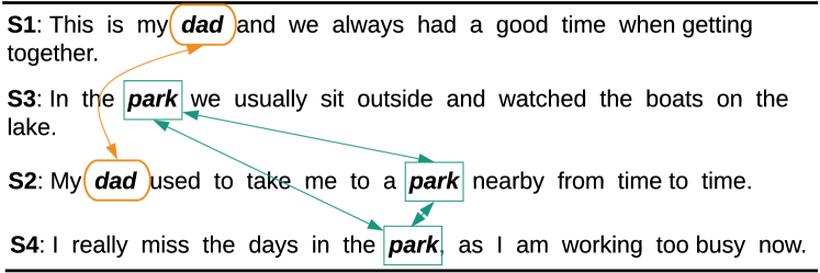
Figure 1: An example of sentence ordering, where the correct order is: S1, S2, S3, S4. S2 is more coherent with S1 than S4, as they share the same entity “dad”.

In this paper, we propose a novel graph-based neural sentence ordering model that adapts the recent graph recurrent network (GRN) Zhang et al. (2018). Inspired by Guinaudeau and Strube Guinaudeau and Strube (2013), we first represent the input set of sentences (paragraph) as a Sentence-Entity graph, where each node represents either a sentence or an entity. Each entity node only connects to the sentence nodes that contain it, and two sentence nodes are linked if they contain the same entities. By doing so, our graph representations are able to model not only the semantic relevance between coherent sentences but also the co-occurrence between sentences and entities. Here we take the example in Figure 1 to illustrate the intuition behind our representations. We can see that the sentences sharing the same entities tend to be semantically close to each other: both the sentences S1 and S2 contain the entity “dad”, and thus they are more coherent than S1 and S4. Compared with the fully-connected graph representations explored previously Cui et al. (2018), our graph representations reduce the noise caused by the edges between irrelevant sentence nodes. Another advantage is that the useful entity information can be fully exploited when encoding the input paragraph. Based on sentence-entity graphs, we then adopt GRN Zhang et al. (2018) to recurrently perform semantic transitions among connected nodes. In particular, we introduce an additional paragraph-level node to assemble semantic information of all nodes during this process, where the resulting paragraph-level representation is beneficial to information transitions among long-distance connected nodes. Moreover, since sentence nodes and entity nodes play different roles, we employ different parameters to distinguish their impacts. Finally, on the basis of the learned paragraph representation, a pointer network is used to produce the order of sentences.

The main contribution of our work lies in introducing GRN into sentence ordering, which can be classified into three sub aspects: 1) We propose a GRN-based encoder for sentence ordering. Our work is the first one to explore such an encoder for this task. Experimental results show that our model significantly outperforms the state-of-the-arts. 2) We refine vanilla GRN by modeling sentence nodes and entity nodes with different parameters. 3) Via plenty of experiments, we verify that entities are very useful in graph representations for sentence ordering.

2 Baseline: ATTOrderNet

In this section, we give a brief introduction to ATTOrderNet, which achieves state-of-the-art performance and thus is chosen as the baseline of our work. As shown in Figure 2, ATTOrderNet consists of a Bi-LSTM sentence encoder, a paragraph encoder based on multi-head self-attention Vaswani et al. (2017), and a pointer network based decoder Vinyals et al. (2015b). It takes a set of input sentences $\boldsymbol{s}=\left[s_{o_{1}},\dots,s_{o_{M}}\right]$ with the order $\boldsymbol{o}=\left[o_{1},\dots,o_{M}\right]$ as input and tries to recover the correct order $\boldsymbol{o}^{*}=\left[o_{1}^{*},\dots,o_{M}^{*}\right]$. Here $M$ denotes the number of the input sentences.

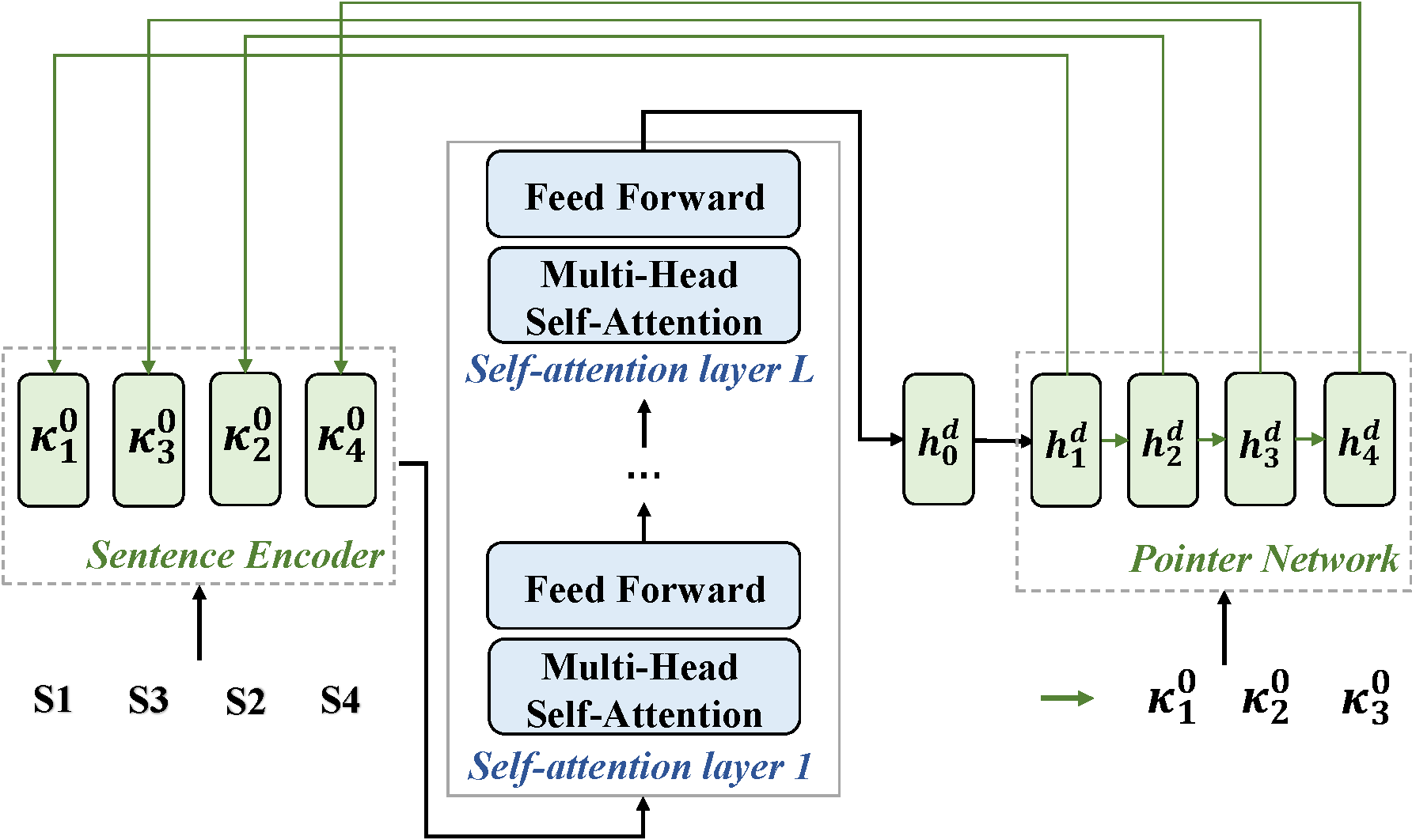
Figure 2: The architecture of ATTOrderNet.

2.1 Sentence Encoding with Bi-LSTM

The Bi-LSTM sentence encoder takes a word embedding sequence ($\boldsymbol{x}_{1},\dots,\boldsymbol{x}_{n}$) of each input sentence $s_{o_{i}}$ to produce its semantic representation. At the $j$-th step, the current states ($\overrightarrow{\boldsymbol{h}}_{j}$ and $\overleftarrow{\boldsymbol{h}}_{j}$) are generated from the previous hidden states ($\overrightarrow{\boldsymbol{h}}_{j-1}$ and $\overleftarrow{\boldsymbol{h}}_{j+1}$) and the current word embedding $\boldsymbol{x}_{j}$ as follows:

$$\overrightarrow{\boldsymbol{h}}_{j}=\text{LSTM}(\overrightarrow{\boldsymbol{h}}_{j-1},\boldsymbol{x}_{j});\overleftarrow{\boldsymbol{h}}_{j}=\text{LSTM}(\overleftarrow{\boldsymbol{h}}_{j+1},\boldsymbol{x}_{j}).$$ (1)

Finally, the sentence representation is obtained by concatenating the last states of the Bi-LSTM in both directions $\boldsymbol{\kappa}^{0}_{o_{i}}=[\overrightarrow{\boldsymbol{h}}_{n};\overleftarrow{\boldsymbol{h}}_{1}]$.

2.2 Paragraph Encoding with Multi-Head Self-Attention Network

The paragraph encoder consists of several self-attention layers followed by an average pooling layer. Given the representations for the input sentences, the initial paragraph representation $\boldsymbol{K}^{0}$ is obtained by concatenating all sentence representations $\boldsymbol{K}^{0}=[\boldsymbol{\kappa}^{0}_{o_{1}},\dots,\boldsymbol{\kappa}^{0}_{o_{M}}]$.

Next, the initial representation is fed into $L$ self-attention layers for the update. In particular, the update for layer $l$ is conducted by

$$\boldsymbol{K}^{l}=\textrm{SelfAtten}_{l}(\boldsymbol{K}^{l-1})\textrm{,}$$ (2)

where $\text{SelfAtten}_{l}$ represents the $l$-th network layer including multi-head self-attention and feed-forward networks. Finally, an average pooling layer is used to generate the final paragraph representation $\boldsymbol{g}$ from the output $K^{L}$ of the last self-attention layer $\boldsymbol{g}=\frac{1}{M}\sum_{i=1}^{M}\boldsymbol{\kappa}^{L}_{i}\textrm{,}$ where $\boldsymbol{\kappa}^{L}_{i}$ is the vector representation of $s_{o_{i}}$.

2.3 Decoding with Pointer Network

After obtaining the final paragraph representation $\boldsymbol{g}$, an LSTM-based pointer network is used to predict the correct sentence order. Formally, the conditional probability of a predicted order $\boldsymbol{o}^{\prime}$ given input paragraph $\boldsymbol{s}$ can be formalized as

$$P(\boldsymbol{o}^{\prime}|\boldsymbol{s}) =\prod_{i=1}^{M}P(o^{\prime}_{i}|\boldsymbol{o}^{\prime}_{<i},\boldsymbol{s})$$ (3)

$$P(o^{\prime}_{i}|\boldsymbol{o}^{\prime}_{<i},\boldsymbol{s}) =\textrm{softmax}(\boldsymbol{v}^{T}\tanh(\boldsymbol{W}\boldsymbol{h}_{i}^{d}+\boldsymbol{U}\boldsymbol{K}^{0})),$$

where $\boldsymbol{v}$, $\boldsymbol{W}$ and $\boldsymbol{U}$ are model parameters. During training, the correct sentence order $\boldsymbol{o}^{*}$ is known, so the sequence of decoder inputs is $\left[\boldsymbol{\kappa}^{0}_{o_{1}^{*}},\dots,\boldsymbol{\kappa}^{0}_{o_{M}^{*}}\right]$. At test time, the decoder inputs correspond to the representations of sentences in the predicted order. For each step $i$, the decoder state is updated recurrently by taking the representation of the previous sentence $\boldsymbol{\kappa}^{0}_{o^{\prime}_{i-1}}$ as the input:

$$\boldsymbol{h}_{i}^{d}=\textrm{LSTM}(\boldsymbol{h}_{i-1}^{d},\boldsymbol{\kappa}^{0}_{o^{\prime}_{i-1}}),$$ (4)

where $\boldsymbol{h}_{i}^{d}$ is the decoder state, and $\boldsymbol{h}_{0}^{d}$ is initialized as the final paragraph representation $\boldsymbol{g}$. The first-step input and initial cell memory are zero vectors.

3 Our Model

In this section, we give a detailed description to our graph-based neural sentence ordering model, which consists of a sentence encoder, a graph neural network based paragraph encoder and a pointer network based decoder. For fair comparison, our sentence encoder and decoder are identical with those of ATTOrderNet. Due to the space limitation, we only describe our paragraph encoder here, which involves graph representations and graph encoding.

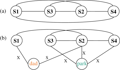
Figure 3: Comparison between (a) a fully-connected graph and (b) our sentence-entity graph for the example in Figure 1. An edge label in (b) corresponds to the syntactic role of an entity in a sentence.

3.1 Sentence-Entity Graph

To take advantage of graph neural network for encoding paragraph, we need to represent input paragraphs as graphs. Different from the fully-connected graph representations explored previously Cui et al. (2018), we follow Guinaudeau and Strube Guinaudeau and Strube (2013) to incorporate entity information into our graphs, where it can serve as additional knowledge and be exploited to alleviate the noise caused by connecting incoherent sentences. To do this, we first consider all nouns of each input paragraph as entities. Since there can be numerous entities for very long paragraphs, we remove the entities that only appear once in the paragraph. As a result, we observe that a reasonable number of entities are generated for most paragraphs, and we will show more details in the experiments.

Then, with the identified entities, we transform the input paragraph into a sentence-entity graph. As shown in Figure 3 (b), our sentence-entity graphs are undirected and can be formalized as $G=(\boldsymbol{V},\boldsymbol{\hat{V}},\boldsymbol{\mathcal{E}})$, where $\boldsymbol{V}$, $\boldsymbol{\hat{V}}$ and $\boldsymbol{\mathcal{E}}$ represent the sentence-level nodes (such as $v_{i}$), entity-level nodes (such as $\hat{v}_{j}$), and edges, respectively. Every sentence-entity graph has two types of edges, where an edge of the first type (SE) connects a sentence and an entity within it. Inspired by Guinaudeau and Strube Guinaudeau and Strube (2013), we set the label for each SE-typed edge based on the syntactic role of the entity in the sentence, which can be either a subject(S), an object(O) or other(X). If an entity appears multiple times with different roles in the same sentence, we pick the highest-rank role according to S$\succ$O$\succ$X. On the other hand, every edge of the second type (SS) connects two sentences that have common entities, and these edges are unlabeled. As a result, sentence nodes are connected to other sentence nodes and entity nodes, while entity nodes are only connected to sentence nodes.

Figure 3 compares a fully-connected graph with a sentence-entity graph for the example in Figure 1. Within the fully-connected graph, there are several unnecessary edges that introduce noise, such as the one connecting S1 and S4. Intuitively, S1 and S4 do not form a coherent context. It is probably because they do not have common entities, especially given the situation that they both share entities with other sentences. In contrast, the sentence-entity graph does not take that edge, thus it does not suffer from the corresponding noise. Another problem with the fully-connected graph is that every node is directly linked to others, thus no information can be obtained based on the graph structure. Conversely, the structure of our sentence-entity graph can provide more discriminating information.

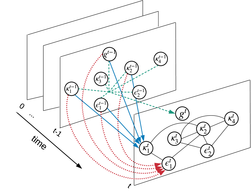
Figure 4: GRN encoding for a sentence-entity graph. The original graph structure is only drawn on step $t$ for being concise.

3.2 Encoding with GRN

To encode our graphs, we adopt GRN Zhang et al. (2018) that has been shown effective in various kinds of graph encoding tasks. GRN is a kind of graph neural network Scarselli et al. (2009) that parallelly and iteratively updates its node states with a message passing framework. For every message passing step $t$, the state update for each node $v_{i}$ mainly involves two steps: a message is first calculated from its directly connected neighbors, then the node state is updated by applying the gated operations of an LSTM step with the newly calculated message. Here we use GRU for updating node states instead of LSTM for better efficiency and fewer parameters.

Figure 4 shows the architecture of our GRN-based paragraph encoder, which adopts a paragraph-level state $\boldsymbol{g}$ in addition to the sentence states (such as $\boldsymbol{\kappa}_{i}$, we follow Section 2.2 to use $\boldsymbol{\kappa}$) and entity states (such as $\boldsymbol{\epsilon}_{j}$). We consider the sentence nodes and the entity nodes as different semantic units, since they contain different amount of information and have different types of neighbors. Therefore, we apply separate parameters and different gated operations to model their state transition processes, both following the two-step message-passing process. To update a sentence state $\boldsymbol{\kappa}_{i}^{t-1}$ at step $t$, messages from neighboring sentence states (such as $\boldsymbol{\kappa}_{i^{\prime}}^{t-1}$) and entity states (such as $\boldsymbol{\epsilon}_{j}^{t-1}$) are calculated via weighted sum:

$$\boldsymbol{m}_{i}^{t} =\sum_{v_{i^{\prime}}\in N_{i}}\boldsymbol{w}_{i,i^{\prime}}\boldsymbol{\kappa}_{i^{\prime}}^{t-1}$$ (5)

$$\boldsymbol{\tilde{m}}_{i}^{t} =\sum_{\hat{v}_{j}\in\tilde{N}_{i}}\boldsymbol{\tilde{w}}_{i,j,l}\boldsymbol{\epsilon}_{j}^{t-1}$$

where $N_{i}$ and $\tilde{N}_{i}$ denote the sets of neighboring sentences and entities of $v_{i}$, respectively. We compute gates $\boldsymbol{w}_{i,j}$ and $\boldsymbol{\tilde{w}}_{i,j,l}$ according to the edge label $l_{i,j}$ (if any) and the two associated node states using a single-layer network with a sigmoid activation. Then, $\boldsymbol{\kappa}_{i}^{t-1}$ is updated by aggregating the messages ($\boldsymbol{m}_{i}^{t}$ and$\ \boldsymbol{\tilde{m}}_{i}^{t}$) and the global state $\boldsymbol{g}^{t-1}$ via

$$\boldsymbol{\xi}_{i}^{t}=[\boldsymbol{s}_{i};\boldsymbol{m}_{i}^{t};\boldsymbol{\tilde{m}}_{i}^{t};\boldsymbol{g}^{t-1}]$$ (6)

$$\boldsymbol{r}_{i}^{t}=\sigma\left(\boldsymbol{W}^{r}\boldsymbol{\xi}_{i}^{t}+\boldsymbol{U}^{r}\boldsymbol{\kappa}_{i}^{t-1}\right)$$

$$\boldsymbol{z}_{i}^{t}=\sigma\left(\boldsymbol{W}^{z}\boldsymbol{\xi}_{i}^{t}+\boldsymbol{U}^{z}\boldsymbol{\kappa}_{i}^{t-1}\right)$$

$$\boldsymbol{u}_{i}^{t}=tanh\left(\boldsymbol{W}^{u}\boldsymbol{\xi}_{i}^{t}+\boldsymbol{U}^{u}\left(\boldsymbol{r}_{i}^{t}\odot\boldsymbol{\kappa}_{i}^{t-1}\right)\right)$$

$$\boldsymbol{\kappa}_{i}^{t}=\left(\boldsymbol{1}-\boldsymbol{z}_{i}^{t}\right)\odot\boldsymbol{u}_{i}^{t}+\boldsymbol{z}_{i}^{t}\odot\boldsymbol{\kappa}_{i}^{t-1}$$

Similarly, at step $t$, each entity state $\boldsymbol{\epsilon}_{j}^{t-1}$ is updated based on its word embedding $\boldsymbol{e}_{j}$, its directly connected sentence nodes (such as $\boldsymbol{\kappa}_{i}^{t-1}$), and the global node $\boldsymbol{g}_{t-1}$:

$$\boldsymbol{\hat{m}}_{j}^{t} =\sum_{v_{i}\in\hat{N}_{j}}\boldsymbol{\hat{w}}_{j,i,l}\boldsymbol{\kappa}_{i}^{t-1}$$ (7)

$$\boldsymbol{\hat{\xi}}_{j}^{t} =[\boldsymbol{e}_{j};\boldsymbol{\hat{m}}_{j}^{t};\boldsymbol{g}^{t-1}]$$

$$\boldsymbol{\hat{r}}_{j}^{t} =\sigma\left(\boldsymbol{\hat{W}}^{r}\boldsymbol{\hat{\xi}}_{i}^{t}+\boldsymbol{\hat{U}}^{r}\boldsymbol{\epsilon}_{i}^{t-1}\right)$$

$$\boldsymbol{\hat{z}}_{j}^{t} =\sigma\left(\boldsymbol{\hat{W}}^{z}\boldsymbol{\hat{\xi}}_{i}^{t}+\boldsymbol{\hat{U}}^{z}\boldsymbol{\epsilon}_{i}^{t-1}\right)$$

$$\boldsymbol{\hat{u}}_{j}^{t} =tanh\left(\boldsymbol{\hat{W}}^{u}\boldsymbol{\hat{\xi}}_{i}^{t}+\boldsymbol{\hat{U}}^{u}\left(\boldsymbol{\hat{r}}_{j}^{t}\odot\boldsymbol{\epsilon}_{i}^{t-1}\right)\right)$$

$$\boldsymbol{\epsilon}_{j}^{t} =\left(\boldsymbol{1}-\boldsymbol{\hat{z}}_{i}^{t}\right)\odot\boldsymbol{\hat{u}}_{i}^{t}+\boldsymbol{\hat{z}}_{i}^{t}\odot\boldsymbol{\epsilon}_{i}^{t-1}$$

Finally, the global state $\boldsymbol{g}^{t-1}$ is updated with the messages from both sentence and entity states via

$$\boldsymbol{\overline{\kappa}}^{t-1} =\frac{1}{M}\sum_{m=1}^{M}\boldsymbol{\kappa}_{m}^{t-1}$$ (8)

$$\boldsymbol{\overline{\epsilon}}^{t-1} =\frac{1}{\hat{M}}\sum_{m=1}^{\hat{M}}\boldsymbol{\epsilon}_{m}^{t-1}$$

$$\boldsymbol{r}_{g}^{t}=\sigma(\boldsymbol{W}^{sr}\boldsymbol{\overline{\kappa}}^{t-1} +\boldsymbol{W}^{er}\boldsymbol{\overline{\epsilon}}^{t-1}+\boldsymbol{U}^{gr}\boldsymbol{g}^{t-1})$$

$$\boldsymbol{z}_{g}^{t}=\sigma(\boldsymbol{W}^{sz}\boldsymbol{\overline{\kappa}}^{t-1} +\boldsymbol{W}^{ez}\boldsymbol{\overline{\epsilon}}^{t-1}+\boldsymbol{U}^{gz}\boldsymbol{g}^{t-1})$$

$$\boldsymbol{u}_{g}^{t}=tanh(\boldsymbol{W}^{su}\boldsymbol{\overline{\kappa}}^{t-1} +\boldsymbol{W}^{eu}\boldsymbol{\overline{\epsilon}}^{t-1}+\boldsymbol{U}^{gu}(\boldsymbol{r}_{g}^{t}\odot\boldsymbol{g}^{t-1}))$$

$$\boldsymbol{g}^{t}=(\boldsymbol{1}-\boldsymbol{z}_{g}^{t}) \odot\boldsymbol{u}_{g}^{t}+\boldsymbol{z}_{g}^{t}\odot\boldsymbol{g}^{t-1},$$

where $\boldsymbol{W}^{*}$ ($*$ $\in$ $\{r,z,u,sr,er,sz,ez,su,eu\}$), $\boldsymbol{U}^{*}$ ($*$ $\in$ $\{r,z,u,gr,gz,gu\}$), $\boldsymbol{\hat{W}}^{*}$ and $\boldsymbol{\hat{U}}^{*}$ ($*\in\{r,z,u\}$) are model parameters, and $\hat{M}$ is the number of entities. In this way, each node absorbs richer contextual information through the iterative encoding process and captures the logical relationships with others. After recurrent state transitions of $T$ iterations, we obtain the final paragraph state $g^{T}$, which will be used to initialize the state $\boldsymbol{h}^{d}_{0}$ of decoder (see Section 2.3).

Model	NIPS Abstract			ANN Abstract			arXiv Abstract			SIND
	Acc	$\tau$	#pm	Acc	$\tau$	#pm	PMR	$\tau$	#pm	PMR	$\tau$	#pm
LSTM+PtrNet $\dagger$	50.87	0.67	2.1M	58.20	0.69	3.0M	40.44	0.72	12.7M	12.34	0.48	3.6M
V-LSTM+PtrNet $\dagger$	51.55	0.72	26.5M	58.06	0.73	28.9M	-	-	-	-	-	-
ATTOrderNet $\dagger$	56.09	0.72	8.7M	63.24	0.73	17.9M	42.19	0.73	23.5M	14.01	0.49	14.4M
F-Graph	56.24	0.72	4.1M	63.45	0.74	9.9M	42.50	0.74	19.6M	14.48	0.50	10.6M
S-Graph	56.67	0.73	4.1M	64.09	0.76	9.9M	43.37	0.74	19.6M	15.15	0.50	10.6M
SE-Graph	57.27*	0.75*	5.0M	64.64*	0.78*	11.5M	44.33*	0.75*	21.3M	16.22*	0.52*	12.2M

Table 1: Main results on the sentence ordering task, where #pm shows the number of parameters, $\dagger$ indicates previously reported scores and * means significant at $p<0.01$ over the F-Graph on each test set. V-LSTM+PtrNet stands for Varient-LSTM+PtrNet. We conduct 1,000 bootstrap tests Koehn (2004) to measure the significance in metric score differences.

4 Experiments

4.1 Setup

Datasets.

We first compare our approach with previous methods on several benchmark datasets.

• NIPS Abstract. This dataset contains roughly 3K abstracts from NIPS papers from 2005 to 2015.

• ANN Abstract. It includes about 12K abstracts extracted from the papers in ACL Anthology Network (AAN) corpus Radev et al. (2016).

• arXiv Abstract. We further consider another source of abstracts collected from arXiv. It consists of around 1.1M instances.

• SIND. It has 50K stories for the visual storytelling task, which is in a different domain from the others. Here we use each story as a paragraph.

For data preprocessing, we first use NLTK to tokenize the sentences, and then adopt Stanford Parser to extract nouns with syntactic roles for the edge labels (S, O or X). For each paragraph, we treat all nouns appearing more than once in it as entities. On average, each paragraph from NIPS Abstract, ANN Abstract, arXiv Abstract and SIND has 5.8, 4.5, 7.4 and 2.1 entities, respectively.

Settings.

Our settings follow Cui et al., Cui et al. (2018) for fair comparison. We use 100-dimension Glove word embeddings. The hidden size of LSTM is 300 for NIPS Abstract and 512 for the others. For our GRN encoders, The state sizes for sentence and entity nodes are set to 512 and 150, respectively. The size of edge embeddings is set to 50. Adadelta Zeiler (2012) is adopted as the optimizer with $\epsilon$ = $10^{-6}$, $\rho$ = $0.95$ and initial learning rate 1.0. For regularization term, we employ L2 weight decay with coefficient $10^{-5}$ and dropout with probability 0.5. Batch size is 16 for training and beam search with size 64 is implemented for decoding.

Contrast Models.

We compare our model (SE-Graph) with the existing state of the arts, including (1) LSTM+PtrNet Gong et al. (2016), (2) Varient-LSTM+PtrNet Logeswaran et al. (2018), and (3) ATTOrderNet Cui et al. (2018). Their major difference is how to encode paragraphs: LSTM+PtrNet uses a conventional LSTM to learn paragraph representation, Varient-LSTM+PtrNet is based on a set-to-sequence framework Vinyals et al. (2015a), and ATTOrderNet adopts self-attention mechanism. Besides, in order to better study the different effects of entities, we also list the performances of two variants of our model: (1) F-Graph. Similar to ATTOrderNet, it uses a fully-connected graph to represent the input unordered paragraph, but adopts GRN rather than self-attention layers to encode the graphs. (2) S-Graph. It is a simplified version of our model by removing all entity nodes and their related edges from the original sentence-entity graphs. Correspondingly, all entity states ($\boldsymbol{\epsilon}$s in Equations 5, 6, 7 and 8) are also removed.

Evaluation Metrics.

Following previous work, we use the following three major metrics:

• Kendall’s tau ($\tau$): It ranges from -1 (the worst) to 1 (the best). Specifically, it is calculated as 1- 2$\times$(number of inversions)/$\binom{M}{2}$, where $M$ denote the sequence length and number of inversions is the number of pairs in the predicted sequence with incorrect relative order.

• Accuracy (Acc): It measures the percentage of sentences whose absolute positions are correctly predicted. Compared with $\tau$, it penalizes results that correctly preserve most relative orders but with a slight shift.

• Perfect Match Ratio (PMR): It considers each paragraph as a single unit and calculates the ratio of exactly matching orders, so no partial credit is given for any incorrect permutations.

Obviously, these three metrics evaluate the quality of sentence ordering from different aspects, and thus their combination can give us a comprehensive evaluation on this task.

4.2 Effect of Recurrent Step $t$

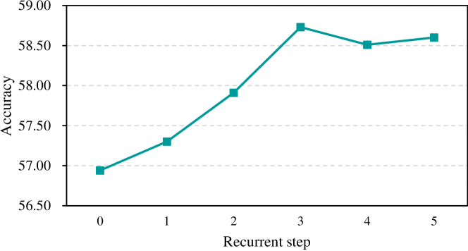
Figure 5: Results on the arXiv Abstract validation set regarding the recurrent steps $t$.

The recurrent step $t$ is an important hyperparameter to our model, thus we choose the validation set of our largest dataset (arXiv Abstract) to study its effectiveness. Figure 5 shows the results. We observe large improvements when increasing $t$ from 0 to 3, showing the effectiveness of our framework. Nevertheless, the increase of $t$ from 3 to 5 does not lead to further improvements while requiring more running time. Therefore, we set $t$=3 for all experiments thereafter.

4.3 Main Results

Table 1 reports the overall experimental results. Our model exhibits the best performance across datasets in different domains, demonstrating the effectiveness and robustness of our model. Moreover, we draw the following interesting conclusions. First, based on the same fully-connncted graph representations, F-Graph slightly outperforms ATTOrderNet on all datasets, even with fewer number of parameters and relatively fewer recurrent steps. This result proves the validity of applying GRN to encode paragraphs. Second, S-Graph shows better performance compared with F-Graph. This confirms the hypothesis that leveraging entity information can reduce the noise caused by connecting incoherent sentences. Third, SE-Graph outperforms S-Graph on all datasets across all metrics. It is because incorporating entities as extra information and modeling the co-occurrence between sentences and entities can further contribute to our neural graph model. Considering that SE-Graph has slightly more parameters than S-Graph, we make further analysis in Section 4.4 to show that the improvement given by SE-Graph is irrelevant to introducing new parameters.

Previous work has indicated that both the first and last sentences play special roles in a paragraph due to their crucial absolute positions, so we also report accuracies of our models on predicting them. Table 2 summarizes the experimental results on arXiv Abstract and SIND, where SE-Graph and its two variants also outperform ATTOrderNet, and particularly, SE-Graph reaches the best performance. Again, both results witness the advantages of our model.

Model	arXiv Abstract		SIND
	head	tail	head	tail
LSTM+PtrNet $\dagger$	90.47	66.49	74.66	53.30
ATTOrderNet $\dagger$	91.00	68.08	76.00	54.42
F-Graph	91.43	68.56	76.53	56.02
S-Graph	91.99	69.74	77.07	56.28
SE-Graph	92.28	70.45	78.12	56.68

Table 2: The ratio of correctly predicting first and last sentences on arXiv Abstract and SIND. $\dagger$ indicates previously reported scores.

4.4 Ablation Study

To investigate the impacts of entities and edges on our model, we adopt SE-Graph and S-Graph for further ablation studies, because both of them exploit entity information. Particularly, we continue to choose arXiv Abstract, the largest among our datasets, to conduct reliable analyses. The results are shown in Table 3, and we have the following observations.

First, shuffling edges significantly hurts the performances of both S-Graph and SE-Graph. The resulting PMR of S-Graph (42.41) is still comparable with the PMR of F-Graph (42.50 as shown in Table 1). Intuitively, shuffling edges can introduce a lot of noise. These facts above indicate that fully-connected graphs are also very noisy, especially because F-Graph takes the same number of parameters as S-Graph. Therefore we can confirm our previous statement again: the entities can help reduce noise. Second, removing edge labels leads to less performance drops than removing or shuffling edges. It is likely because some labels can be automatically learned by our graph encoder. Nevertheless, the labels still provide useful information. Third, there are slight decreases for S-Graph and SE-Graph, if we only remove 10% entities. Removing entities is a way to simulate syntactic parsing noise, as our entities are obtained by the parsing results. This indicates the robustness of our model against potential parsing accuracy drops on certain domains, such as medical and chemistry. On the other hand, randomly removing 50% entities causes significant performance drops. As the model size still remains unchanged, this shows the importance of introducing entities. Particularly, the result of removing 50% entities for SE-Graph is slightly worse than original model of S-Graph, demonstrating that SE-Graph’s improvement over S-Graph is not derived from simply introducing more parameters. Finally, share parameters illustrates the effect of making both GRNs (Equations 6 and 7) to share parameters. The result shows a drastic decrease on final performance, which is quite reasonable because entity nodes play fundamentally different roles from sentence nodes. Consequently, it is intuitive to model them separately.

5 Related work

Sentence Ordering.

Previous work on sentence ordering mainly focused on the utilization of linguistic features via statistical models Lapata (2003); Barzilay and Lee (2004); Barzilay and Lapata (2005, 2008); Elsner and Charniak (2011); Guinaudeau and Strube (2013). Especially, the entity based models Barzilay and Lapata (2005, 2008); Guinaudeau and Strube (2013) have shown the effectiveness of exploiting entities for this task. Recently, the studies have evolved into neural network based models, such as window network Li and Hovy (2014), neural ranking model Chen et al. (2016), hierarchical RNN-based models Gong et al. (2016); Logeswaran et al. (2018), and ATTOrderNet Cui et al. (2018). Compared with these models, we combine the advantages of modeling entities and GRN, obtaining state-of-the-art performance. Even without entity information, our model variant based on fully-connected graphs still shows better performance than the previous state-of-the-art model, indicating that GRN is a stronger alternative for this task.

Model	S-Graph		SE-Graph
	Acc	PMR	Acc	PMR
Original	58.06	43.37	58.91	44.33
Shuffle edges	57.06	42.41	57.46	42.84
Remove edge labels	—	—	58.51	43.96
Remove 50% entities	57.57	42.83	57.84	43.18
Remove 10% entities	57.79	43.26	58.67	44.17
Share parameters	—	—	55.30	40.31

Table 3: Ablation study of our graph structure on arXiv Abstract, where Share Parameters means employing the same parameters to update entity and sentence nodes.

Graph Neural Networks in NLP.

Recently, graph neural networks have been shown successful in the NLP community, such as modeling semantic graphs Beck et al. (2018); Song et al. (2018a, 2019), dependency trees Marcheggiani and Titov (2017); Bastings et al. (2017); Song et al. (2018b), knowledge graphs Wang et al. (2018) and even sentences Zhang et al. (2018); Xu et al. (2018). Particularly, Zhang et al., Zhang et al. (2018) proposed GRN to represent raw sentences by building a graph structure of neighboring words and a sentence-level node. Their model exhibit satisfying performance on several classification and sequence labeling tasks. Our work is in line with theirs for the exploration of adopting GRN on NLP tasks. To our knowledge, our work is the first attempt to investigate GRN on solving a paragraph coherence problem.

6 Conclusion

We have presented a neural graph-based model for sentence ordering. Specifically, we first introduce sentence-entity graphs to model both the semantic relevance between coherent sentences and the co-occurrence between sentences and entities. Then, GRN is adopted on the built graphs to encode input sentences by performing semantic transitions among connected nodes. Compared with the previous state-of-the-art model, ours is capable of reducing the noise brought by relationship modeling between incoherent sentences, but also fully leveraging entity information for paragraph encoding. Extensive experiments on several benchmark datasets prove the superiority of our model over the state-of-the-art and other baselines.

References

- Barzilay and Lapata [2005] Regina Barzilay and Mirella Lapata. Modeling local coherence: An entity-based approach. In ACL, pages 141–148, 2005.
- Barzilay and Lapata [2008] Regina Barzilay and Mirella Lapata. Modeling local coherence: An entity-based approach. Computational Linguistics, 34(1):1–34, 2008.
- Barzilay and Lee [2004] Regina Barzilay and Lillian Lee. Catching the drift: Probabilistic content models, with applications to generation and summarization. In NAACL, pages 113–120, 2004.
- Barzilay et al. [2002] Regina Barzilay, Noemie Elhadad, and Kathleen R. McKeown. Inferring strategies for sentence ordering in multidocument news summarization. Journal of Artificial Intelligence Research, 17:35–55, 2002.
- Bastings et al. [2017] Joost Bastings, Ivan Titov, Wilker Aziz, Diego Marcheggiani, and Khalil Sima’an. Graph convolutional encoders for syntax-aware neural machine translation. In EMNLP, pages 1957–1967, 2017.
- Beck et al. [2018] Daniel Beck, Gholamreza Haffari, and Trevor Cohn. Graph-to-sequence learning using gated graph neural networks. In ACL, pages 273–283, 2018.
- Chen et al. [2016] Xinchi Chen, Xipeng Qiu, and Xuanjing Huang. Neural sentence ordering. CoRR, abs/1607.06952, 2016.
- Cui et al. [2018] Baiyun Cui, Yingming Li, Ming Chen, and Zhongfei Zhang. Deep attentive sentence ordering network. In EMNLP, pages 4340–4349, 2018.
- Elsner and Charniak [2011] Micha Elsner and Eugene Charniak. Extending the entity grid with entity-specific features. In ACL, pages 125–129, 2011.
- Galanis et al. [2012] Dimitrios Galanis, Gerasimos Lampouras, and Ion Androutsopoulos. Extractive multi-document summarization with integer linear programming and support vector regression. In COLING, pages 911–926, 2012.
- Gong et al. [2016] Jingjing Gong, Xinchi Chen, Xipeng Qiu, and Xuanjing Huang. End-to-end neural sentence ordering using pointer network. CoRR, abs/1611.04953, 2016.
- Guinaudeau and Strube [2013] Camille Guinaudeau and Michael Strube. Graph-based local coherence modeling. In ACL, pages 93–103, 2013.
- Koehn [2004] Philipp Koehn. Statistical significance tests for machine translation evaluation. In EMNLP, pages 388–395, 2004.
- Lapata [2003] Mirella Lapata. Probabilistic text structuring: Experiments with sentence ordering. In ACL, 2003.
- Li and Hovy [2014] Jiwei Li and Eduard H. Hovy. A model of coherence based on distributed sentence representation. In EMNLP, pages 2039–2048, 2014.
- Logeswaran et al. [2018] Lajanugen Logeswaran, Honglak Lee, and Dragomir R. Radev. Sentence ordering and coherence modeling using recurrent neural networks. In AAAI Conference on Artificial Intelligence, pages 5285–5292, 2018.
- Marcheggiani and Titov [2017] Diego Marcheggiani and Ivan Titov. Encoding sentences with graph convolutional networks for semantic role labeling. In EMNLP, pages 1506–1515, 2017.
- Radev et al. [2016] Dragomir R. Radev, Mark Thomas Joseph, Bryan R. Gibson, and Pradeep Muthukrishnan. A bibliometric and network analysis of the field of computational linguistics. JASIST, 67(3):683–706, 2016.
- Scarselli et al. [2009] Franco Scarselli, Marco Gori, Ah Chung Tsoi, Markus Hagenbuchner, and Gabriele Monfardini. The graph neural network model. IEEE Trans. Neural Networks, 20(1):61–80, 2009.
- Song et al. [2018a] Linfeng Song, Yue Zhang, Zhiguo Wang, and Daniel Gildea. A graph-to-sequence model for amr-to-text generation. In ACL, pages 1616–1626, 2018.
- Song et al. [2018b] Linfeng Song, Yue Zhang, Zhiguo Wang, and Daniel Gildea. N-ary relation extraction using graph-state lstm. In EMNLP, pages 2226–2235, 2018.
- Song et al. [2019] Linfeng Song, Daniel Gildea, Yue Zhang, Zhiguo Wang, and Jinsong Su. Semantic neural machine translation using amr. CoRR, abs/1902.07282, 2019.
- Vaswani et al. [2017] Ashish Vaswani, Noam Shazeer, Niki Parmar, Jakob Uszkoreit, Llion Jones, Aidan N. Gomez, Lukasz Kaiser, and Illia Polosukhin. Attention is all you need. In NIPS, pages 6000–6010, 2017.
- Vinyals et al. [2015a] Oriol Vinyals, Samy Bengio, and Manjunath Kudlur. Order matters: Sequence to sequence for sets. In ICLR, 2015.
- Vinyals et al. [2015b] Oriol Vinyals, Meire Fortunato, and Navdeep Jaitly. Pointer networks. In NIPS, pages 2692–2700, 2015.
- Wang et al. [2018] Zhichun Wang, Qingsong Lv, Xiaohan Lan, and Yu Zhang. Cross-lingual knowledge graph alignment via graph convolutional networks. In EMNLP, pages 349–357, 2018.
- Xu et al. [2018] Kun Xu, Lingfei Wu, Zhiguo Wang, Yansong Feng, Michael Witbrock, and Vadim Sheinin. Graph2seq: Graph to sequence learning with attention-based neural networks. CoRR, abs/1804.00823, 2018.
- Yu et al. [2018] Adams Wei Yu, David Dohan, Minh-Thang Luong, Rui Zhao, Kai Chen, Mohammad Norouzi, and Quoc V. Le. Qanet: Combining local convolution with global self-attention for reading comprehension. In ICLR, 2018.
- Zeiler [2012] Matthew D. Zeiler. ADADELTA: an adaptive learning rate method. CoRR, abs/1212.5701, 2012.
- Zhang et al. [2018] Yue Zhang, Qi Liu, and Linfeng Song. Sentence-state lstm for text representation. In ACL, pages 317–327, 2018.