Rényi divergences from Euclidean quenches

Abstract

We study the generalisation of relative entropy, the Rényi divergence $D_{\alpha}(\rho||\rho_{\beta})$ in 2$d$ CFTs between an excited state density matrix $\rho$, created by deforming the Hamiltonian, and the thermal density matrix $\rho_{\beta}$. Using the path integral representation of this quantity as a Euclidean quench, we obtain the leading contribution to the Rényi divergence for deformations by scalar primaries and by conserved holomorphic currents in conformal perturbation theory. Furthermore, we calculate the leading contribution to the Rényi divergence when the conserved current perturbations have inhomogeneous spatial profiles which are versions of the sine-square deformation (SSD). The dependence on the Rényi parameter ($\alpha$) of the leading contribution have a universal form for these inhomogeneous deformations and it is identical to that seen in the Rényi divergence of the simple harmonic oscillator perturbed by a linear potential. Our study of these Rényi divergences shows that the family of second laws of thermodynamics, which are equivalent to the monotonicity of Rényi divergences, do indeed provide stronger constraints for allowed transitions compared to the traditional second law.

1 Introduction

The application of ideas from information theory has led to important insights in quantum field theory, holography and black hole physics. The most well studied measure is that of entanglement entropy which is defined as the von-Neumann entropy of the reduced density matrix on a spatial region. Entanglement entropy and its holographic realization in terms of the minimal surface Ryu:2006bv has been the key ingredient for the recent developments in AdS/CFT and black holes. Another concept which has recently received attention is the relative entropy of two density matrices which is defined as

$$S(\rho_{1}||\rho_{2})={\rm Tr}(\rho_{1}\log\rho_{1})-{\rm Tr}(\rho_{1}\log\rho_{2})~{}.$$ (1)

Relative entropy assigns a positive number given two density matrices and therefore can be used as a measure of distance in the space of density matrices. It was introduced in the holographic context in Blanco:2013joa and has subsequently found several applications Bousso:2014sda ; Jafferis:2015del . For an introduction to information theoretic measures and their applications in quantum field theory see Witten:2018lha .

Just as the Rényi entropies are a one parameter generalisation of the von-Neumann entropy, relative entropy also admits one parameter generalisations. The focus of this paper is the generalization known as Rényi divergence, also known as the Petz entropy PETZ198657 . This is defined as

$$D_{\alpha}(\rho_{1}||\rho_{2})=\frac{{\rm sgn}(\alpha)}{\alpha-1}\log{\rm Tr[\rho^{\alpha}_{1}\rho_{2}^{1-\alpha}]}~{},$$ (2)

where $\rho_{1},\rho_{2}$ are normalized density matrices. This quantity forms an important distance measure in information theory. In Bernamonti:2018vmw Rényi divergence between a state $\rho$ deformed from the thermal state $\rho_{\beta}$ at the temperature $\beta$ with respect to a given Hamiltonian $H$ was used to study additional second law like constraints which can govern the out of equilibrium state $\rho$ as it evolves to the thermal state $\rho_{\beta}$ by the Hamiltonian $H$. The excited state $\rho$ considered in Bernamonti:2018vmw is also a thermal state but under a deformed Hamiltonian $H_{\rm def}=H+\mu{\cal O}$ where ${\cal O}$ is the deforming operator. For this class of excited states, Bernamonti:2018vmw showed that one can evaluate the Rényi divergences using its path integral as a Euclidean quench. The Euclidean quench was also used to develop a method to evaluate Rényi divergences holographically. In the cases where $H$ describes a $2$-dimensional conformal field theory and ${\cal O}$ a conformal primary of dimensions $\Delta<1$, it was shown that there are indeed situations where constraints are stronger than the conventional second law. These additional constraints resulted from the monotonicity of Rényi divergences.

In this paper we study more properties of Rényi divergences in $2$-dimensional conformal field theory. The formulation of Rényi divergence as a Euclidean quench presents us with the interesting problem of calculating a new class of generalized partition functions

$$\mathcal{Z}_{\alpha}(\tau,\mu)=\text{Tr}\left[q^{\alpha H_{\rm def}(\mu)}q^{(1-\alpha)H_{\rm CFT}}\right].$$ (3)

Here, $H_{\rm def}(\mu)=H_{\rm CFT}+\mu\mathcal{O}$. After a review of the formulation of Rényi divergence as a Euclidean quench, we re-visit the evaluation of the leading contribution to Rényi divergences for excited states created by deforming the Hamiltonian by a scalar primary of weight $\Delta$. We obtain an analytical expression for the Rényi divergence in terms of an infinite series. The representation in terms of infinite series is obtained for all values of $\Delta$ provided the integral resulting from conformal perturbation theory is regulated. For the case $\Delta=1$ we obtain a closed form expression in terms of known functions.

When $\mathcal{O}$ commutes with the Hamiltonian, as is the case with conserved current deformations, the above quantity can be calculated from the knowledge of the deformed partition function $\text{Tr}\left[q^{H_{\rm def}(\alpha\mu)}\right]$. We consider the cases of $U(1)$, the stress tensor and the spin-3 current deformations. We obtain the generalised partition function (3) partition function for these cases in the closed form by considering the perturbative expansion in the coupling $\mu$. For carrying out the conformal perturbation theory we used the methods developed earlier in Datta:2014ska ; Datta:2014uxa ; Datta:2014zpa . The prescription adopted for carrying out the integrals that arise in conformal perturbation theory ensure that each integral is finite despite the fact the conformal dimension of the current is such that $\Delta\geq 1$. These methods enable us to evaluate the Rényi divergences, $D_{\alpha}(\rho||\rho_{\beta})$, where $\rho$ is the excited state obtained by adding conserved currents to the Hamiltonian.

When $\mathcal{O}$ does not commute with $H_{\rm CFT}$, calculating $\mathcal{Z}_{\alpha}$ is not straightforward. The effective Hamiltonian $H_{\rm eff}$, defined as $q^{H_{\rm eff}}=q^{\alpha H_{\rm def}(\mu)}q^{(1-\alpha)H_{\rm CFT}}$, then involves an appropriate re-summation of the Baker-Campbell-Hausdorff series. We note that ${H_{\rm eff}}$ is also the Floquet Hamiltonian governing the dynamics if the system is evolved alternatively using $H_{\rm CFT}$ and $H_{\rm def}$. Some progress in finding closed form expressions for $H_{\rm eff}$ has been made in floquet:replica . To render the problem tractable we work with the situation that the deforming operator $\mathcal{O}$ is still constructed from conserved currents, but $\mu$ acquires a spatial profile. Taking the spatial directions to be compact and choosing periodic functions in space one can obtain deforming operators $\mathcal{O}$ which do not commute with Hamiltonian $H_{\rm{CFT}}$. For the case of the stress tensor, a special class of deformations was considered earlier in ishibashi:ssd ; wen:floquet ; wen:ssd ; vishwanath:ssd ; chitra:ssd called sine-square deformation (SSD). This name is derived from the fact the spatial dependence of the envelope function is a sine-squared profile. We generalise this envelope function introducing a parameter $\mu$ which controls the amplitude of the deformation. The deforming operator is then proportional to combination of Virasoro generators, $L_{1}+L_{-1}$. We also generalise to the cases when the deforming operator is constructed from higher spin currents. We call these the higher spin SSD deformations. Analogous to the Virasoro case, the deforming operator is given by $V^{(s)}_{-k}+V^{(s)}_{k}$, where $k$ is the mode number of the the spin-$s$ current and $V^{(s)}$ is the generator of higher spin symmetries.

We set up Hamiltonian perturbation theory in $\mu$ and evaluate the generalised partition function (3) and the corresponding Rényi divergences. For the SSD and its higher spin generalization we find that the $\alpha$ dependence of the leading contribution to the Rényi divergence takes the following universal form

$$D_{\alpha}(\rho_{\mu}||\rho_{\beta})=\mu^{2}\frac{\sinh(\frac{\pi(\alpha-1)k\beta}{L})\sinh(\frac{\pi\alpha k\beta}{L})}{(\alpha-1)}f(\beta,L)+O(\mu^{4})~{}.$$ (4)

Here $k$ is the mode number of the deforming operator, $V^{(s)}_{-k}+V^{(s)}_{k}$ and $L$ is the size of the spatial circle. We also show that this dependence on $\alpha$ is remarkably identical to the Rényi divergence of the simple harmonic oscillator deformed by a linear potential. For the case of the simple harmonic oscillator, the Rényi divergence in (4) is exact to all orders in $\mu$ and $\frac{\beta}{L}$ is replaced by $\omega\beta$ where $\omega$ is the frequency of the oscillator. We show the universality in Rényi divergence is the consequence of the same nature of commutation relations of the deforming operator with the undeformed Hamiltonian. These operators satisfy the Heisenberg algebra.

Armed with these results for Rényi divergences, we examine the constraints for non-equilibrium transitions arising from generalized second laws put forward in Bernamonti:2018vmw . We see that for open systems, indeed monotonicity of Rényi divergences place more constraints on allowed transitions than the conventional second law. These observations generalise those found in Bernamonti:2018vmw . Due to the analytical nature of our result we are able to translate the constraints from the generalised second laws to domains in the deforming parameter $\mu$ for which non-equilibrium transitions are allowed. These domains turn out to be more restrictive than those allowed by the traditional second law.

The organization of the paper is as follows. In section 2, we review the formulation of Rényi divergences in terms of the Euclidean quench and also discuss some of its properties. In section 3, we evaluate Rényi divergences for deformations due to scalar primaries of dimension $\Delta$. In section 4, we consider situations with $\mu$ constant and the deforming operators are the $U(1)$ currents, stress tensor, spin-3 currents and evaluate the corresponding Rényi divergences in closed form using conformal perturbation theory. In section 5, we first consider the case of the simple Harmonic oscillator deformed by the linear potential and show using the path integral that the Rényi divergence is exactly given by (4). We then evaluate the Rényi divergences of the SSD deformation and its higher spin analogues using Hamiltonian perturbation theory and how that to the leading order the $\alpha$ dependence of the Rényi divergence is given by the universal form in (4). In section 6, we use our results and show that generalized second laws for non-equlibrium transitions based on Rényi divergences do indeed place additional constrains compared to the conventional second law. Section 7 contains our conclusions. Appendix A contains details of conformal perturbation theory for spin-2 and spin-3 deformation. Appendix B and Appendix C contains evaluation of partition functions and the details of the Hamiltonian perturbation theory for the SSD deformation and its higher spin generalizations.

2 Rényi divergence as Euclidean quench

In this section we review the evaluation of Rényi divergences using its path integral representation as an Euclidean quench put forward in Bernamonti:2018vmw . The Rényi divergence between two density matrices $\rho$ and $\rho_{\beta}$ is defined as

$$D_{\alpha}(\rho||\rho_{\beta})=\frac{1}{\alpha-1}\log\frac{\rm Tr[\rho^{\alpha}\rho_{\beta}^{1-\alpha}]}{\rm Tr{[\rho]}^{\alpha}~{}\rm Tr{[\rho_{\beta}]}^{1-\alpha}}~{}.$$ (5)

Here, $\rho$ is an excited state obtained by deforming the Hamiltonian corresponding to the thermal density matrix $\rho_{\beta}$. Therefore, the path integral representation of $\rho_{\beta}$ is the path integral of the conformal field theory with action $S_{\rm CFT}$ over a cylinder of circumference $\beta$. We write this formally

$$\rho_{\beta}=\int[d\phi]\exp(-S_{\rm CFT}(\phi))~{},$$ (6)

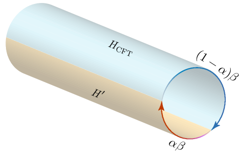
Figure 1: The Euclidean quench setup for Rényi divergence.

In the operator language the thermal density matrix can be written as

$$\rho_{\beta}=e^{-\beta H_{\rm CFT}},$$ (7)

where $H_{\rm CFT}$ is the Hamiltonian which generates translations along the thermal circle. The deformed density matrix $\rho$ is then defined by the path integral

$$\rho=\int[d\phi]\exp\left[-S_{\rm CFT}(\phi)-\int dzd\bar{z}\,\mu\,{\cal O}_{\Delta}(z,\bar{z})\right],$$ (8)

where ${\cal O}_{\Delta}(z,\bar{z})$ is a conformal primary of weight $(h,\bar{h})$ with $\Delta=h+\bar{h}$. In the Hamiltonian form, the excited state $\rho$ can be thought of a thermal state defined with respect to a new Hamiltonian given by

$$H^{\prime}=H_{\rm CFT}+\mu{\cal O}_{\Delta}~{},$$ (9)

and therefore $\rho=e^{-\beta H^{\prime}}$.

Now, the path integral representation of the trace appearing in the numerator of the definition of the Rényi divergence in (5) can be summarised in Fig. 1. Essentially we sew the regions of the path integral given in (6) and (8). Thus the entire path integral can be thought of as performing the path integral on the thermal cylinder with the Hamiltonian $H_{\rm CFT}$ deformed by the operator ${\cal O}$ coupled to a time dependent source given by

$$\mu(\tau)=(\theta(\tau)-\theta(\tau-\alpha\beta))\mu~{}.$$ (10)

Here $\theta(\tau)$ refers to the Heaviside step function defined by

$$\theta(\tau)=\left\{\begin{array}[]{ll}1&\mbox{ for }\;\tau\geq 0,\\ 0&\mbox{ for }\;\tau<1.\end{array}\right.$$ (11)

Since the deformation is turned on at $\tau=0$ and turned off at $\tau=\alpha\beta$, this formulation of the Rényi divergence is also called the Euclidean quench. The factors in the denominator in (5) can be evaluated using the path integral (6) and (8).

It is clear from this formulation for evaluating Rényi divergences that we are restricted to the specific class of excited states which are obtained by deforming the original Hamiltonian $H_{\rm CFT}$. As in Bernamonti:2018vmw we wish to think of these as excited states within the theory in which the evolution is determined by $H_{\rm CFT}$. Also the path integral formulation allows the evaluation of the Rényi divergence for the range $0\leq\alpha<1$.

The work Bernamonti:2018vmw focused on deformation by relevant scalar primaries, in this paper we first revisit these deformations. We then focus on deformation by conserved currents and also evaluate Rényi divergences when the perturbations in $\mu$ have inhomogenous spatial profiles which specifically correspond to the sine-squared deformation (SSD).

Before we go ahead let us also recall a few properties Rényi divergences van_Erven_2014 . One simple check we perform in the next section is that we verify these properties are true for all the cases for which we have evaluated the Rényi divergences.

1. Positivity: $D_{\alpha}\geq 0$.

2. Monotonicity in $\alpha$: $D_{\alpha_{1}}\geq D_{\alpha_{2}}$ for $\alpha_{1}>\alpha_{2}$.

3. Continuity in $\alpha$.

4. Concavity: $(1-\alpha)D_{\alpha}$ is concave in $\alpha$.

5. Relation to relative entropy in the $\alpha\rightarrow 1$ limit:

   $$D_{1}(\rho||\rho_{\beta})={\rm Tr}(\rho\log\rho)-{\rm Tr}(\rho\log\rho_{\beta}).$$ (12)

   Furthermore it can be shown that relative entropy can be written in terms of the differences in free energies of the density matrices $\rho$ and $\rho_{\beta}$

   $$D_{1}(\rho||\rho_{\beta})=\beta(F(\rho)-F(\rho_{\beta})).$$ (13)

   It is important to realise that in this equation, the free energy of the excited state is given by

   $$F(\rho)={\rm Tr}[\hat{\rho}H]+{\rm Tr}[\hat{\rho}\log\hat{\rho}].$$ (14)

   Note that the expectation value of the energy is that of the undeformed Hamiltonian in the excited state $\rho$ and $\hat{\rho}$ is the normalized density matrix given by

   $$\hat{\rho}=\frac{\rho}{{\rm Tr}[\rho]}$$ (15)

   The definition of $F(\rho_{\beta})$ is the same as that of (14) with $\rho$ replaced by $\rho_{\beta}$.

It is useful to obtain an expression for the free energy of excited state in terms of the partition function the excited state. Consider the un-normalized density matrix of the excited state which is given by

$$\rho=e^{-\beta(H-\mu{\cal O})}.$$ (16)

where ${\cal O}^{\prime}$ is the operator which corresponds to the deformation in the Hamiltonian picture. From this definition (16) it is easy to see that

$${\rm Tr}[H\hat{\rho}]=\frac{\mu}{\beta}\frac{\partial}{\partial\mu}\log({\rm Tr}[\rho])-\frac{\partial}{\partial\beta}\log({\rm Tr}[\rho]),$$ (17)

Note that on the LHS $\hat{\rho}$ refers to the normalized density matrix and $H$ refers to the undeformed Hamiltonian. We also have the equation

$$\frac{1}{\beta}{\rm Tr}(\hat{\rho}\log\hat{\rho})=-T\frac{\partial}{\partial T}(T\log{\rm Tr}[\rho]).$$ (18)

Both the equations (17) and (18) are functions of the deformed partition function $\mathcal{Z}[\mu]={\rm Tr}[\rho]$. The free energy of the unperturbed CFT is given by

$$F(\rho_{\beta})=-\frac{1}{\beta}\log{\rm Tr}[\rho_{\beta}]=-\frac{\pi cL}{6\beta^{2}}.$$ (19)

Now using (17), (18) and (19), it can be seen that the difference in free energy (14) can be expressed entirely in terms of the partition function of the excited state $\mathcal{Z}[\mu]=\text{Tr}[\rho]$. Therefore, the relative entropy is

$$D_{1}(\rho||\rho_{\beta}) = \beta(F(\rho)-F(\rho_{\beta})),$$

$$= \mu\frac{\partial}{\partial\mu}\log{\rm Tr}[\rho]-\log{\rm Tr}[\rho]+\frac{\pi cL}{6\beta}.$$

Additionally, using $\rho_{\beta}=e^{-\beta H}$ and $\rho=e^{-\beta(H+\mu\mathcal{O})}$ and the Golden-Thompson inequality, $\text{Tr}[e^{A}e^{B}]\geq\text{Tr}[e^{A+B}]$, we obtain that the Rényi divergence (5) is bounded from above by the following combination of the deformed and undeformed partition functions

$$D_{\alpha}(\rho||\rho_{\beta})\leq\frac{1}{\alpha-1}\log\frac{\mathcal{Z}[\alpha\mu]}{\mathcal{Z}[\mu]^{\alpha}\mathcal{Z}[0]^{1-\alpha}},\quad\text{where }\mathcal{Z}[\mu]\equiv\text{Tr}[{e^{-\beta(H+\mu\mathcal{O})}}].$$ (21)

for $0\leq\alpha<1$. This inequality is saturated if and only if the deforming operator $\mathcal{O}$ commutes with the Hamiltonian.

3 Deformations by scalar primaries

In this section we revisit the evaluation of the Rényi divergences for which the excited state is that obtained by a scalar primary ${\cal O}$ of weight $\Delta$ to the quadratic order in the amplitude. This problem was addressed in Bernamonti:2018vmw where the integral resulting from conformal perturbation theory was evaluated numerically and for $\Delta<\frac{1}{2}$, the integral was written in terms of a series. In this section we show that the Rényi divergences can be written as a series for all $\Delta$. Further more for the case of $\Delta=1$, we obtain the Rényi divergences in closed form.

Let us consider the Euclidean quench by a scalar primary, the action is deformed by

$$S_{\rm CFT}\mapsto S_{\rm CFT}+\mu\int d^{2}w[\theta(\tau)-\theta(\tau-\alpha\beta)]{\cal O}(w,\bar{w})~{}.$$ (22)

The leading contribution to the quenched partition function begins at the quadratic order in $\mu$ and is given by

$$\log{\rm Tr}(\rho^{\alpha}\rho^{(1-\alpha)})=\frac{\pi cL}{6\beta}+\mu^{2}\int_{0}^{\alpha\beta}\int_{0}^{\alpha\beta}d\tau_{1}d\tau_{2}\int_{-\infty}^{\infty}\int_{-\infty}^{\infty}d\sigma_{1}d\sigma_{2}\langle{\cal O}(w_{1},\bar{w}_{1}){\cal O}(w_{2},\bar{w}_{2})\rangle+\cdots$$ (23)

The normalized two point function of the primary on the cylinder is given by

$$\langle{\cal O}(w_{1},\bar{w}_{1}){\cal O}(w_{2},\bar{w}_{2})\rangle=\left(\frac{\pi}{\beta}\right)^{2\Delta}\left(\frac{1}{\sinh\frac{\pi}{\beta}(w_{1}-w_{2})\sinh\frac{\pi}{\beta}(\bar{w}_{1}-\bar{w}_{2})}\right)^{\Delta}.$$ (24)

After a change of variable and simple manipulations we obtain

$$\log{\rm Tr}(\rho^{\alpha}\rho^{(1-\alpha)})=\frac{\pi cL}{6\beta}+\frac{\pi L}{\beta}\left(\frac{\pi}{\beta}\right)^{(2\Delta-4)}I(\Delta,\alpha)+\cdots,$$ (25)

where

$$I(\alpha,\Delta)=2^{\Delta-2}\int_{0}^{2\pi\alpha}dp\int_{0}^{\infty}d\sigma\frac{2(2\pi\alpha-p)}{(\cosh\sigma-\sqrt{1-\epsilon^{2}}\cos p)^{\Delta}}.$$ (26)

We have cut off the second spatial integral to a size of length $L$. After a change of variables we have performed the integrals over one of the temporal directions. The integral is regulated following Bernamonti:2018vmw . Using (5), the Rényi divergence is then given by

$$D_{\alpha}(\rho||\rho_{\beta})=\mu^{2}\frac{\pi L}{\beta}\left(\frac{\pi}{\beta}\right)^{(2\Delta-4)}\frac{I(\alpha,\Delta)-\alpha(1,\Delta)}{\alpha-1}+O(\mu^{3}).$$ (27)

We now evaluate the integral in (26) by expanding the denominator using the binomial expansion

$$I(\alpha,\Delta)=2^{\Delta-2}\sum_{n=0}^{\infty}\frac{\Gamma(\Delta+n)}{\Gamma(\Delta)\Gamma(n+1)}(1-\epsilon^{2})^{\frac{n}{2}}\int_{0}^{2\pi\alpha}dp\int_{0}^{\infty}d\sigma\frac{2(2\pi\alpha-p)(\cos p)^{n}}{(\cosh\sigma)^{n+\Delta}}.$$

For a finite $\epsilon$, this expansion is uniformly convergent and we have interchanged the sum and the integral. Now the functions that occur in the integral are elementary and we can integrate term by term. We obtain

$$I(\alpha,\Delta) = I(\alpha,\Delta)_{\text{even}}+I(\alpha,\Delta)_{\text{odd}},$$ (29)

$$I(\alpha,\Delta)_{\text{even}} = 2^{2\Delta-3}\sum_{m=0}^{\infty}\Gamma_{m}(\Delta)\,(1-\epsilon^{2})^{m}\left[\sum_{k=0}^{m-1}\binom{2m}{k}s(m-k)+\binom{2m}{m}2\pi^{2}\alpha^{2}\right],$$

$$I(\alpha,\Delta)_{\text{odd}} = 2^{2\Delta-3}\sum_{m=1}^{\infty}\Gamma_{m-\frac{1}{2}}(\Delta)\,(1-\epsilon^{2})^{\frac{2m-1}{2}}\sum_{k=0}^{m-1}4\binom{2m-1}{k}s(m-k-\tfrac{1}{2}),$$

where we have defined the quantities $s(x)=\sin^{2}[2\pi\alpha x]/x^{2}$ and $\Gamma_{m}(\Delta)=\Gamma(m+\Delta/2)^{2}/(\Gamma(2m+1)\Gamma(\Delta))$.

The integral is convergent for $0<\Delta<1$, therefore we can set $\epsilon=0$ and we can plot the Rényi divergences given by (27) and (29) In figures 2(a) and 2(b), we have plotted these Rényi divergences for various values of $\Delta$ for 1000 terms in the series. It can be seen that the properties discussed in section 2 hold. We checked the convergence of the series by evaluating the Rényi divergences by taking different the number of terms in the series. For instance changing the number of terms from 800 to 1000 results in changes of less than equal to $0.04$ to the Rényi divergences. The changes kept decreasing as we increased the number of terms. We have also seen by using the ratio test to a series which bounds the one given in (29), that the sum is convergent for any $\Delta$ given a finite $\epsilon$. In (Bernamonti:2018vmw, , Appendix A, equation A.19) a series form of the integral was obtained for strictly $\epsilon=0$ and was valid for $0<\Delta<1/2$, the series we have incorporates the cut off and is convergent for any $\Delta$ given a finite $\epsilon$.

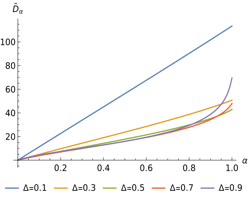
(a)

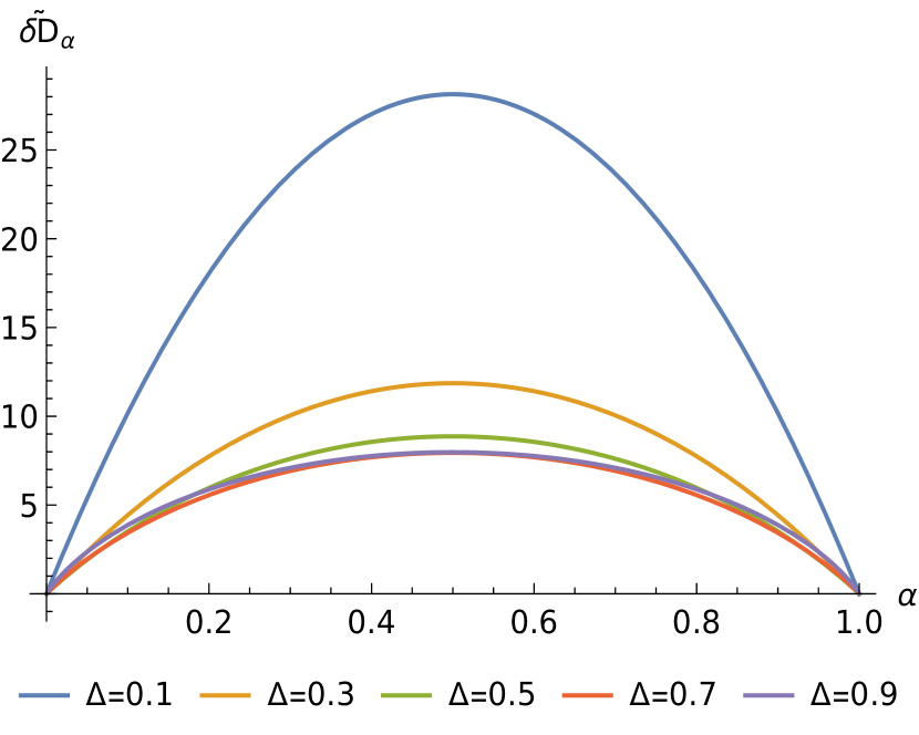
(b)

Figure 2: (Left) Plot of $\tilde{D}_{\alpha}=[\mu^{2}\frac{\pi L}{\beta}(\frac{\pi}{\beta})^{(2\Delta-4)}]^{-1}D_{\alpha}(\rho_{1}||\rho_{2})$ vs $\alpha$. (Right) Plot of $(1-\alpha)\tilde{D}_{\alpha}(\rho_{1}||\rho_{2})$ vs $\alpha$ . In both the plots the values of $\Delta$ for the curves decrease from $0.1$ to $0.9$ from top to bottom. We have taken 1000 terms in the series given in (29).

As a check of our method of integration, we consider the case of $\Delta=1$, for which the integral can be obtained in terms of known functions for $\epsilon=0$. We perform the spatial integral first

$$\int_{0}^{\infty}d\sigma\frac{1}{\cosh\sigma-\cos p}=2\frac{\tan^{-1}(\cot\frac{p}{2})}{\sin p}=\frac{\pi-p}{\sin p}.$$ (30)

Note that we have chosen the branch so that the resulting integral is positive for $p$ in the range $0$ to $2\pi\alpha$. The temporal integral is given by

$$I(\alpha,1)=\int_{0}^{2\pi\alpha}F(p)dp,\qquad\qquad F(p)=\frac{(2\pi\alpha-p)(\pi-p)}{\sin p}.$$ (31)

This integrand is obviously divergent at $p=0$, we can regulate this integral by shifting the contour and considering

$$I(\alpha,1)=\lim_{\epsilon\rightarrow 0}\int_{0}^{2\pi\alpha}\frac{1}{2}(F(p+i\epsilon)+F(p-i\epsilon))dp.$$ (32)

Performing this integral and then evaluating the Rényi divergence we obtain

$$D_{\alpha}(\rho,\rho_{\beta}) = \mu^{2}\frac{\beta L}{\pi}\frac{1}{4(\alpha-1)}\left[i\pi^{3}(2\alpha-1)+2i\pi(2\alpha-1)\left(-4{\rm Li}_{2}(e^{2\mathrm{i}\pi\alpha})+{\rm Li}_{2}(e^{4i\pi\alpha})\right)\right.$$ (33)

$$\hskip 85.35826pt\left.+16{\rm Li}_{3}(e^{2i\pi\alpha})-2{\rm Li}_{3}(e^{4{i}\pi\alpha})-14\zeta(3)\right].$$

Note that though the result in (33) is not manifestly real, it can be seen real by examining the numerical values of the function in the figures 3(a) and 3(b).

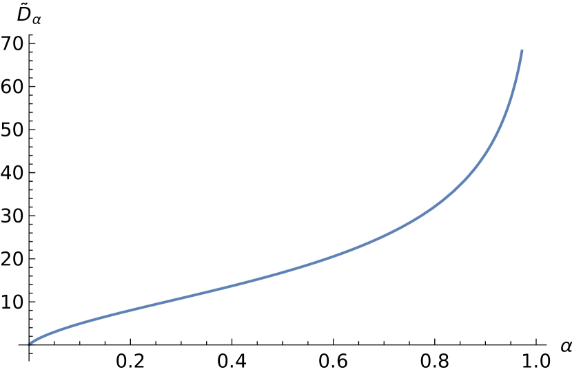
(a)

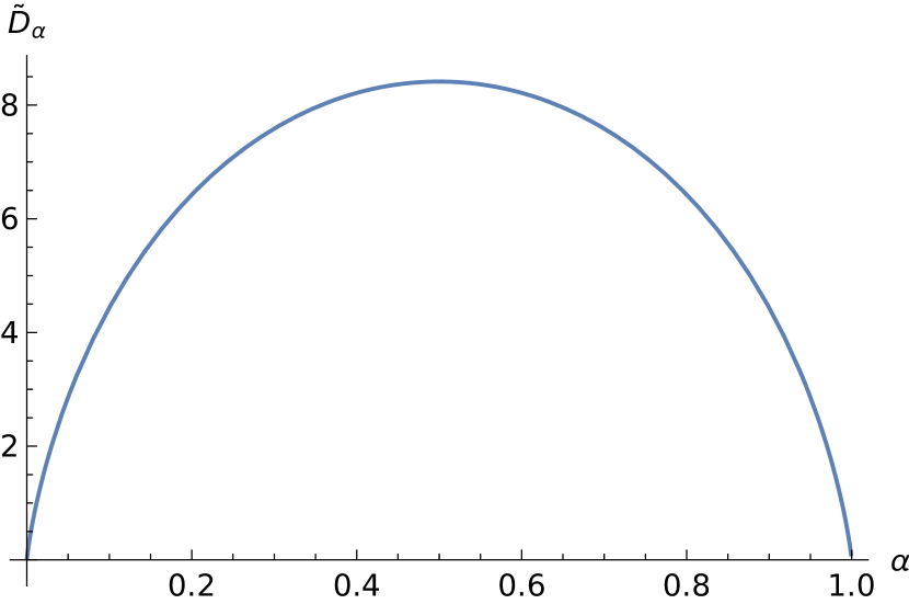
(b)

Figure 3: (Left) Plot of $\tilde{D}_{\alpha}=\frac{1}{\mu^{2}(\beta L/\pi)}D_{\alpha}(\rho_{1}||\rho_{2})$ vs $\alpha$. (Right) Plot of $(1-\alpha)\tilde{D}_{\alpha}(\rho_{1}||\rho_{2})$ vs $\alpha$

We can use the closed form answer at $\Delta=1$ given in (33) to check the efficiency of the series obtained in (Bernamonti:2018vmw, , Appendix A, equation (A.19)) extrapolated to $\Delta=1$. First we note the normalizations of the integral in (26) and that in Bernamonti:2018vmw are related by $I(\alpha,\Delta)_{\rm ours}=2^{\Delta-3}I_{\rm theirs}$. Let us call the Rényi divergence obtained by the series for $\Delta=1$ in (29) as ‘series 1’ and that obtained in Bernamonti:2018vmw after taking into account the normalizations, ‘series 2’. In figure 4(a) we have plotted the closed form result for the Rényi divergences from (33) and ‘series 1’ and ‘series 2’ for 1000 terms in the series. In figure 4(b) we plot the differences between the closed from result and ‘series 1’ and ‘series 2’ taking 1000 terms. As expected the closed form result is always larger, however we can see the ‘series 1’ obtained is this paper has smaller differences and therefore converges faster to the closed form answer.

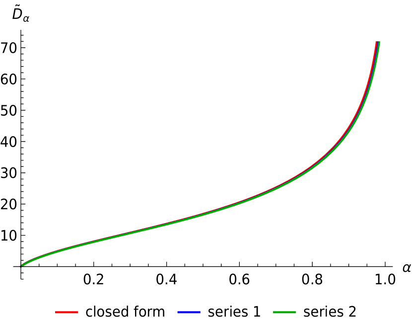
(a)

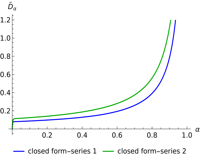
(b)

Figure 4: (Left) Plots of $\tilde{D}_{\alpha}=\frac{1}{\mu^{2}(\beta L/\pi)}D_{\alpha}(\rho_{1}||\rho_{2})$ vs $\alpha$ for $\Delta=1$. The closed form in (33) is shown as a continuous curve, ‘series 1’ constructed in this paper and ‘series 2’ of Bernamonti:2018vmw are as dashed curves of yellow and green respectively. We have taken 1000 terms from each of the series. (Right) Plots of $\tilde{D}_{\alpha}$ for differences: (closed form $-$ ‘series 1’) and (closed form $-$ ‘series 2’). It is seen that the series (29) constructed has smaller differences to the closed form result.

As another consistency check, we consider the limit $\alpha\to 1$ of the integral $I(\alpha,\Delta)$ with $\Delta<1$ for covergence so that we can set $\epsilon=0$. The integral then becomes

$$I(1,\Delta)=2^{\Delta-2}\int_{0}^{2\pi}dp\int_{0}^{\infty}\frac{2(2\pi-p)}{(\cosh\sigma-\cos p)^{\Delta}}.$$ (34)

We can now compare this integral done in (Berenstein:2014cia, , equation (13)) for $d=2$ (also obtained for conformal perturbation theory)

$$C_{\Delta} = \int_{-\infty}^{\infty}d\tau\int_{0}^{\pi}d\theta~{}{\rm Vol}(S_{0})~{}\frac{1}{2^{\Delta}(\cosh\tau-\cos\theta)^{\Delta}}.$$ (35)

This integral was evaluated with the result

$$C_{\Delta} = \pi^{\frac{3}{2}}2^{1-\Delta}\left[\frac{\Gamma(1-\Delta)\Gamma(\frac{\Delta}{2})}{\Gamma(1-\frac{\Delta}{2})^{2}\Gamma(\frac{1}{2}+\frac{\Delta}{2})}\right].$$ (36)

Now using the following identity for every integer $n$

$$\int_{0}^{2\pi}dp(2\pi-p)(\cos p)^{n}=2\pi\int_{0}^{\pi}d\theta(\cos p)^{n}.$$ (37)

and comparing the integrals in (34) and (35), we expect

$$I(1,\Delta)=4^{\Delta-1}\pi C_{\Delta}~{}.$$ (38)

Let us now evaluate $I(1,\Delta)$. From the series representation of the integral (29) is easy to see that the result is

$$I(1,\Delta) = 2^{2\Delta-2}\sum_{m=0}^{\infty}\frac{\Gamma\left(\frac{2m+\Delta}{2}\right)^{2}}{\Gamma(2m+1)\Gamma(\Delta)}\binom{2m}{m}\pi^{2}=\frac{2^{(2\Delta-2)}\pi^{2}\Gamma(1-\Delta)\Gamma(\frac{\Delta}{2})^{2}}{\Gamma(\frac{2-\Delta}{2})^{2}\Gamma(\Delta)}.$$ (39)

Evaluating the ratio from (35) and (39) we indeed see that the ratio is precisely as expected and is given by

$$\frac{I(1,\Delta)}{C_{\Delta}}=4^{\Delta-1}\pi~{}.$$ (40)

We also see that, as expected for $\alpha=1$ the result in (39) is $2^{\Delta-3}$ times the result evaluated using the series in Bernamonti:2018vmw .

4 Homogenous deformations by conserved currents

In this section we study Rényi divergence when the source $\mu$ is spatially uniform and the operator ${\cal O}$ are conserved currents. Thus the deformation we consider are

$$S_{\rm{CFT}}(\phi)\mapsto S_{\rm{CFT}}(\phi)+\mu\int d^{2}z\left({\cal O}(z)+{\bar{\cal O}}(\bar{z})\right)$$ (41)

In the subsequent subsections we consider ${\cal O}(z)$ to be spin-1, spin-2, spin-3 currents and show that the Rényi divergences for these deformations can be obtained in closed form to all orders in conformal perturbation theory. Note that all these operators have dimensions $\Delta\geq 1$. It was noted in Bernamonti:2018vmw , that for primaries with conformal dimensions $\Delta\geq 1$ and $h=\bar{h}$, there are divergences in conformal perturbation theory. On the contrary, we will see that in the case of holomorphic currents the prescription developed in Datta:2014ska ; Datta:2014uxa ; Datta:2014zpa to evaluate the integrals that occur in conformal perturbation theory leads to finite answers for Rényi divergences.

4.1 $U(1)$ current

Let us consider the following deformation of the CFT action by a $U(1)$ current

$$S_{\rm{CFT}}(\phi)\mapsto S_{\rm{CFT}}(\phi)+\mu\int d^{2}z\left({j}(z)+{\bar{j}}(\bar{z})\right).$$ (42)

The $U(1)$ current admits the following OPE

$$j(z)j(w)\sim-\frac{\kappa}{(z-w)^{2}},$$ (43)

where $\kappa$ is the level of the current algebra. We focus on the holomorphic perturbation. The analysis for the anti-holomorphic perturbation proceeds identically and we can then add its contribution. The correlators of the anti-holomorphic $U(1)$ current with the holomorphic current factorise except for contact-terms which involve delta functions. In the prescription of doing the resulting integrals we ignore all such contact-terms (see Datta:2014zpa for details). Therefore the contribution from the anti-holomorphic sector can be taken into account by doubling the contribution of the holomorphic sector.

To proceed let us study the leading correction to the partition function: we evaluate

$${\rm Tr}(\rho)=\mathcal{Z}[\mu]=\int[D\phi]\exp\left(-S[\phi]-\mu\int d^{2}w\,j(w)\right)~{}.$$ (44)

This path integral is evaluated on a cylinder of length $L$ with circumference $\beta$. $w$ is the co-ordinate on the cylinder which is related to the co-ordinate on the plane by the map $z=e^{{2\pi w}/{\beta}}~{}.$ Expanding the partition function as a series in $\mu$, we obtain

$$\frac{\mathcal{Z}[\mu]}{\mathcal{Z}[0]}=1-\mu\int d^{2}w\langle j(w)\rangle+\frac{\mu^{2}}{2}\int d^{2}w_{1}d^{2}w_{2}\langle j(w_{1})j(w_{2})\rangle+\cdots.$$ (45)

Here the expectation values refer to correlators evaluated on the cylinder. Since $j(w)$ is a conformal primary, is expectation value on the cylinder vanishes. The two-point function of the currents on the cylinder is given by

$$\langle j(w_{1})j(w_{2})\rangle=-\kappa\left(\frac{\pi}{\beta}\right)^{2}\frac{1}{\sinh^{2}\frac{\pi}{\beta}(w_{1}-w_{2})}.$$ (46)

To perform the integral we adopt the prescription developed in Datta:2014ska ; Datta:2014uxa ; Datta:2014zpa . The spatial integrals are done first followed by the temporal integrals. Furthermore the last spatial integral is cut off by the length $L$ of cylinder and it gives rise to the extensivity of the free energy. Let us see this in detail for the $\mu^{2}$ term in (45)

$$-\frac{1}{2}\mu^{2}\kappa\int_{0}^{\beta}d\tau_{2}\int_{-L/2}^{L/2}d\sigma_{2}\int_{0}^{\beta}d\tau_{1}\int_{-\infty}^{\infty}d\sigma_{1} \left(\frac{\pi}{\beta}\right)^{2}\frac{1}{\sinh^{2}\frac{\pi}{\beta}(\sigma_{1}-\sigma_{2}+i(\tau_{1}-\tau_{2}))}$$

$$=\pi\kappa\mu^{2}L\beta~{}.$$ (47)

Here we have used $w=\sigma+i\tau$ where $\sigma$ is the non-compact spatial direction and $\tau$, the compact temporal direction. Notice that in this prescription the integrals over the temporal directions are trivial. This is because performing the spatial integral first picks out the conserved charge. As we will see, the fact that the temporal integrals are trivial plays an important role for evaluating when this deformation occurs as a Euclidean quench.

For the $U(1)$ current, all $n$-point functions (on the cylinder) where $n$ is odd vanish, and for even $n$ they factorise into two-point functions. Using this and the integral in (4.1) we can exponentiate all the terms in the expansion (45) to obtain

$$\mathcal{Z}[\mu] = \mathcal{Z}[{0}]\times\exp{(2\pi\kappa\mu^{2}L\beta)}.$$ (48)

Here we have included the contributions from the anti-holomorphic sector. The undeformed CFT partition function is easily evaluated using the high temperature limit, since the length of the cylinder is large. Thus we have

$${\rm Tr}[\rho_{\beta}]=\mathcal{Z}[0]=\exp\left(\frac{\pi cL}{6\beta}\right),$$ (49)

where $c$ is the central charge of the CFT. Combining (48) and (49), we obtain at high temperatures

$${\rm Tr}[\rho]=\mathcal{Z}[\mu]=\exp{\left(\frac{\pi cL}{6\beta}+2\pi\kappa\mu^{2}L\beta\right)}.$$ (50)

This result is also consistent with the modular transformation of the torus partition function in the Hamiltonian formalism. The grand-canonical partition function at low temperatures receives dominant contribution from the uncharged vacuum

$$\mathcal{Z}(\tau,\nu)=\text{Tr}\left[q^{L_{0}-c/24}{\bar{q}}^{\bar{L}_{0}-c/24}y^{J_{0}}{\bar{y}}^{\bar{J}_{0}}\right],\qquad\mathcal{Z}_{\rm low}(\tau,\nu)\approx\exp\left(\frac{\pi c\beta}{6L}\right),$$ (51)

here, $q=e^{2\pi i\tau}$, $y=e^{2\pi i\nu}$ and we chose $\tau=i\beta/L$. Under modular transformations, the above partition function transforms as

$$\mathcal{Z}\left(\frac{a\tau+b}{c\tau+d},\frac{\nu}{c\tau+d}\right)=\exp\left[\frac{ic\pi\kappa\nu^{2}}{c\tau+d}-\frac{ic\pi\kappa\bar{\nu}^{2}}{c\bar{\tau}+d}\right]~{}\mathcal{Z}(\tau,\nu).$$ (52)

Using the S-modular transformation, we can obtain the high temperature behaviour of the partition function

$$\mathcal{Z}_{\rm high}(\tau,\nu)\approx\exp{\left(\frac{\pi cL}{6\beta}+{2\pi\kappa\nu^{2}L\over\beta}\right)}.$$ (53)

Upon identifying $\nu=\mu\beta$, this agrees precisely with the result (50) obtained using the Lagrangian/path-integral formalism. This provides a verification of the integration prescription being used here.

Let us now turn to the Euclidean quench, the deformation is now given by

$$S_{\rm{CFT}}(\phi)\mapsto S_{\rm{CFT}}(\phi)+\mu\int d^{2}z[\theta(\tau)-\theta(\tau-\alpha\beta)]\left({j}(z)+{\bar{j}}(\bar{z})\right).$$ (54)

Evaluating the path integral with this action results in ${\rm Tr}[\rho^{\alpha}\rho_{\beta}^{1-\alpha}]$. It is easy to carry out the integrations using the prescription just described. Since the temporal integrals are trivial, performing the two temporal integrals in the case of the Euclidean quench just results in the replacement $\beta^{2}\mapsto\alpha^{2}\beta^{2}$. Therefore the result for the partition function of the quenched theory is given by

$${\rm Tr}(\rho^{\alpha}\rho_{\beta}^{1-\alpha})=\exp{\left(\frac{\pi cL}{6\beta}+2\pi\kappa\alpha^{2}\mu^{2}L\beta\right)}.$$ (55)

Note that due to the triviality of the temporal integrals, the result for the Euclidean quench can be easily obtained from the knowledge of the deformed partition function (50); equivalently this causes a rescaling of the coupling $\mu\mapsto\alpha\mu$. We will see that this property is true for all uniform holomorphic deformations. In the Hamiltonian version this fact can be seen as follows. The partition function for the Euclidean quench setup is

$${\rm Tr}(\rho^{\alpha}\rho_{\beta}^{1-\alpha})=\text{Tr}\left[q^{\alpha(L_{0}-{c\over 24}+{\nu\over\tau}J_{0})}{\bar{q}}^{\alpha(\bar{L}_{0}-{c\over 24}+{\bar{\nu}\over\bar{\tau}}J_{0})}q^{(1-\alpha)(L_{0}-{c\over 24})}{\bar{q}}^{(1-\alpha)(\bar{L}_{0}-{c\over 24})}\right].$$ (56)

Now since $[L_{0},J_{0}]=0$, the product of the operator exponentials can be trivially simplified to yield

$${\rm Tr}(\rho^{\alpha}\rho_{\beta}^{1-\alpha})=\text{Tr}\left[q^{L_{0}-{c\over 24}+{\alpha\nu\over\tau}J_{0}}{\bar{q}}^{\bar{L}_{0}-{c\over 24}+{\alpha\bar{\nu}\over\bar{\tau}}J_{0}}\right]=\text{Tr}\left[q^{L_{0}-{c\over 24}}{\bar{q}}^{\bar{L}_{0}-{c\over 24}}y^{\alpha J_{0}}{\bar{y}}^{\alpha\bar{J}_{0}}\right].$$ (57)

Comparing this to (51) this is a simple rescaling of the chemical potential, $\nu\mapsto\alpha\nu$, and this is also reflected in (55). This feature is universally true for all deformations that commute with the Hamiltonian. This aspect turns out to be very different when we deal with inhomogenous deformations or deformations by primary operators.

Now using (49), (50) and (55) in the definition of Rényi divergence (5) we obtain

$$D_{\alpha}(\rho||\rho_{\beta})=2\pi\alpha\mu^{2}\kappa L\beta.$$ (58)

It is easy to see that this simple linear function in $\alpha$ satisfies all the properties of Rényi divergences listed in Section 2 (for $\kappa>0$).

4.2 Stress tensor

Next we consider the deformation by the stress tensor

$$S_{\rm{CFT}}(\phi)\mapsto S_{\rm{CFT}}(\phi)+\mu\int d^{2}z\left({T}(z)+{\bar{T}}(\bar{z})\right).$$ (59)

As we have seen from the $U(1)$ deformation, the first step is to study the deformed partition function. In Datta:2014zpa , it was seen that using that such a deformation of a CFT defined on a torus leads to a shift in the temperature. This was seen till the quadratic order in perturbation theory where the resulting integrals was carried out by the same prescription of performing the spatial integrals first and then the temporal integrals. Here, we will verify that the deformation given in (59) on the cylinder indeed shifts the temperature to the fourth order in perturbation theory.

Let us begin by considering the expansion of the partition function to $O(\mu^{2})$. We first focus only on the perturbation by the holomorphic stress tensor $T(z)$. As mentioned for the $U(1)$ current, the correlators between the holomorphic stress tensor and its anti-holomorphic counterpart factorise with the exception of delta-function contact terms. Our integration prescription ignores all contact terms and, as before, the anti-holomorphic contribution can be accounted for by doubling the contribution of the holomorphic sector. Till the second order in conformal perturbation theory, we have

$$\log\frac{\mathcal{Z}[\mu]}{\mathcal{Z}[0]} = -\mu\int d^{2}w_{1}\langle T(w_{1})\rangle+\frac{\mu^{2}}{2}\int d^{2}w_{1}d^{2}w_{2}\langle T(w_{1})T(w_{1})\rangle$$

$$-\frac{\mu^{2}}{2}\left(\int d^{2}w_{1}\langle T(w_{1})\rangle\right)^{2}+\cdots.$$

To evaluate the correlators on the cylinder we use the following relation satisfied by the stress tensor under conformal transformation

$$T(w)=\Big{(}\frac{dz}{dw}\Big{)}^{2}T(z)+\frac{c}{12}\{z,w\}$$ (61)

and

$$\{z,w\}=\frac{2z^{\prime\prime\prime}z^{\prime}-3z^{\prime\prime^{2}}}{2z^{\prime^{2}}},$$ (62)

is the Schwarzian of the transformation. We can take $z,w$ are the co-ordinates on the plane and the cylinder which are related by the map

$$z=\exp\left(2\pi\frac{w}{\beta}\right)~{}.$$ (63)

Using this, the 1-point and 2-point functions of the stress tensor on the cylinder are given by

$$\langle T(\omega)\rangle = \frac{c}{12}\Big{(}-\frac{2\pi^{2}}{\beta^{2}}\Big{)},$$ (64)

$$\langle T(\omega_{1})T(\omega_{2})\rangle = \frac{c}{2}\Big{(}\frac{\pi}{\beta}\Big{)}^{4}\Big{[}\frac{1}{\sinh[\pi/\beta(\omega_{2}-\omega_{1})]}\Big{]}^{4}+4\Big{(}\frac{\pi}{\beta}\Big{)}^{4}\Big{(}\frac{c}{12}\Big{)}^{2}~{}.$$

We now have to perform the integrals over the cylinder. Performing the integral for the 1-point function is trivial, it just involves multiplying the 1-point function with the volume of the cylinder $\beta L$. The first non-trivial integral occurs at the quadratic order, it involves the 2-point function

$$\int_{0}^{\beta}d\tau_{1}\int_{0}^{\beta}d\tau_{2}\int_{-\frac{L}{2}}^{\frac{L}{2}}d\sigma_{2}\int_{-\infty}^{\infty}d\sigma_{1}\frac{c}{2}\Big{(}\frac{\pi}{\beta}\Big{)}^{4}\Big{[}\frac{1}{\sinh[\pi/\beta(w_{2}-w_{1})]}\Big{]}^{4}=\frac{2cL\pi^{3}}{3\beta}~{}.$$ (65)

where $w_{i}=\sigma_{i}+i\tau_{i}$. We have used the same recipe to perform the integrals as in the $U(1)$ case. Note that the disconnected term involving the square of the one point function cancels with the constant term which arises from the Schwarzian transformation in (64). This ensures that the free energy is extensive. The result for the partition function to $O(\mu^{2})$ is given by

$$\log\frac{\mathcal{Z}[\mu]}{\mathcal{Z}[0]}=\frac{\pi cL}{6\beta}\left(2\pi\mu+(2\pi\mu)^{2}+\cdots\right)~{}.$$ (66)

Here we have included the contribution from the anti-holomorphic sector.

We have performed the perturbative expansion to $O(\mu^{4})$. The details of the integrals involved are provided in Appendix A.1. The final result to this order is given by

$$\log(\mathcal{Z}[\mu])=\frac{\pi cL}{6\beta}\left(1+2\pi\mu+(2\pi\mu)^{2}+(2\pi\mu)^{3}+(2\pi\mu)^{4}+\cdots\right).$$ (67)

In the above, the high temperature limit of the undeformed CFT partition function has been used

$$\log\mathcal{Z}[0]=\log{\rm Tr}(\rho_{\beta})=\frac{\pi cL}{6\beta}.$$ (68)

On examining the series in (67) it is easy to note that the perturbed partition function can be obtained by shifting the temperature

$$\beta\rightarrow\beta^{\prime}=\beta(1-2\pi\mu).$$ (69)

Thus the partition function is given by

$$\log(\mathcal{Z}[\mu])=\log({\rm Tr}\rho)=\frac{\pi cL}{6\beta(1-2\pi\mu)}.$$ (70)

This is because the prescription of performing the spatial integrals first picks out the conserved charge. For the stress tensor deformation, the conserved charge is the original Hamiltonian (or energy) itself. Therefore, the stress tensor deformation can be thought of as a shift in temperature. This observation also indicates that the range of $\mu$ is restricted to

$$\mu<\frac{1}{2\pi}.$$ (71)

This constraint enforces positivity of the rescaled effective temperature, $\beta^{\prime}$, from equation (69).

Now we can address the Euclidean quench with the above ingredients; the deformation is given by

$$S_{\rm{CFT}}(\phi)\mapsto S_{\rm{CFT}}(\phi)+\mu\int d^{2}z[\theta(\tau)-\theta(\tau-\alpha\beta)]\left({T}(z)+{\bar{T}}(\bar{z})\right).$$ (72)

Going through the steps of expanding the path integral with this deformation in powers of $\mu$ and performing the resulting integrals we arrive at

$$\log\left[{\rm Tr}(\rho^{\alpha}\rho_{\beta}^{1-\alpha})\right]=\frac{\pi cL}{6\beta}\left(1+2\pi\alpha\mu+(2\pi\alpha\mu)^{2}+(2\pi\alpha\mu)^{3}+(2\pi\alpha\mu)^{4}+\cdots\right).$$ (73)

Note that the coupling $\mu$ is replaced by $\alpha\mu$ in the expansion. The reason for this is the same as that observed for the $U(1)$ deformation. Performing the integrals over the spatial co-ordinates first renders the integrations over the temporal co-ordinates trivial and therefore each temporal integral gets multiplied by a factor of $\alpha$ resulting in the expression in (73). Again, the same reasoning holds to all orders in perturbation theory and therefore we obtain

$$\log\left[{\rm Tr}(\rho^{\alpha}\rho_{\beta}^{1-\alpha})\right]=\frac{\pi cL}{6\beta(1-2\pi\alpha\mu)}.$$ (74)

We can now evaluate the Rényi divergences, substituting (68), (70) and (74) into the definition (5), we obtain

$$D_{\alpha}(\rho||\rho_{\beta})=\frac{\pi cL}{6\beta}\frac{4\pi^{2}\alpha\mu^{2}}{(1-2\pi\mu)(1-2\pi\alpha\mu)}.$$ (75)

We can easily check that the above result for the Rényi divergence satisfies the first 4 properties listed in Section 1. It is instructive to check the relation to the relative entropy at $\alpha=1$. In this limit the Rényi divergence becomes

$$D_{1}(\rho||\rho_{\beta})=\frac{\pi cL}{6\beta}\frac{4\pi^{2}\mu^{2}}{(1-2\pi\mu)^{2}}.$$ (76)

It can be verified that the difference in free energies of the excited state $\rho$ and the state $\rho_{\beta}$ using (2) results precisely in (76). This check not only confirms that the relation in (13) holds but also the fact that the undeformed Hamiltonian $H$ determines dynamics.

4.3 Spin-3

Our final example is the deformation by the spin-3 current, $W(z)$

$$S_{\rm{CFT}}(\phi)\mapsto S_{\rm{CFT}}(\phi)+\mu\int d^{2}z\left({W}(z)+{\bar{W}}(\bar{z})\right)~{}.$$ (77)

Such a deformation was studied in Datta:2014ska ; Datta:2014uxa ; Datta:2014zpa to evaluate higher spin corrections to entanglement entropy. In Datta:2014ska , the corrections to the partition function to $O(\mu^{2})$ was also evaluated.

We restrict our attention to the free boson CFT, but it will be clear from our analysis that the evaluation of Rényi divergences can be extended any CFT which admits ${\cal W}_{3}$ within its chiral-algebra. Consider $N$ complex free bosons $\phi_{i}$ which obey the OPE

$$\bar{\phi}_{i}(z,\bar{z})\phi^{j}(w,\bar{w})\sim-\delta^{j}_{i}\log|z-w|^{2}.$$ (78)

This theory admits a spin-3 current conserved current which is given by

$$W(z)=\sqrt{\frac{5}{12\pi^{2}}}\sum_{i=1}^{\frac{c}{2}}:(\partial^{2}\bar{\phi}_{i}(z)\partial\phi_{i}(z)-\partial\bar{\phi}_{i}(z)\partial^{2}\phi_{i}(z)):~{}.$$ (79)

This current is a conformal primary and its leading OPE is given by

$$W(z)W(0)\sim-\frac{5c}{6\pi^{2}z^{6}}+\cdots,$$ (80)

where $c=2N$. Let us again focus on only the holomorphic correction to the partition function. To order $\mu^{4}$ we have the following expansion

$$\log\frac{\mathcal{Z}[\mu]}{\mathcal{Z}[0]}=\, \frac{\mu^{2}}{2}\int d^{2}w_{1}d^{2}w_{2}\langle W(w_{1})W(w_{2})\rangle$$ (81)

$$+\frac{\mu^{4}}{4!}\left[\int d^{2}w_{1}d^{2}w_{2}d^{2}w_{3}d^{2}w_{4}\langle W(w_{1})W(w_{2})W(w_{3})W(w_{3})\rangle\right.$$

$$\qquad\quad\left.-3\left(\int d^{2}w_{1}d^{2}w_{2}\langle W(w_{1})W(w_{2})\rangle\right)^{2}\right]+\cdots.$$

The correlators involving an odd number of insertions of $W$’s vanish. We follow the same prescription to evaluate the integrals as discussed for the $U(1)$ current and the spin-2 deformation. The correlators can be evaluated by Wick contractions; on the cylinder they are given by

$$\langle W(w_{1})W(w_{2})\rangle = -\frac{5c}{6\pi^{2}}\left(\frac{\pi}{\beta\sinh\frac{\pi}{\beta}(w_{1}-w_{2})}\right)^{6},$$ (82)

$$\langle W(w_{1})W(w_{2})W(w_{3})W(w_{4})\rangle = \frac{25c^{2}}{36\pi^{4}}\left(\frac{\pi^{2}}{\beta^{2}\sinh\frac{\pi}{\beta}(w_{1}-w_{2})\sinh\frac{\pi}{\beta}(w_{3}-w_{4})}\right)^{6}$$

$$\left[1+\tfrac{18}{c}\eta+\tfrac{75}{c}\eta^{2}+(2+\tfrac{54}{c})\eta^{3}+9(1+\tfrac{2}{c})\eta^{4}+6\eta^{5}+\eta^{6}\right]~{}.$$

where $\eta$ is the related to the cross ratio by

$$\eta=x+\frac{1}{x}-2,\qquad x=\frac{\sinh\frac{\pi}{\beta}(w_{1}-w_{3})\sinh\frac{\pi}{\beta}(w_{2}-w_{4})}{\sinh\frac{\pi}{\beta}(w_{1}-w_{4})\sinh\frac{\pi}{\beta}(w_{2}-w_{3})}.$$ (83)

We can perform the integrals in the expansion (81) using the same prescription discussed earlier for the spin-1 and spin-2 deformations. The result for the integral which occurs at the $\mu^{2}$ order is

$$\int_{0}^{\beta}d\tau_{2}\int_{0}^{\beta}d\tau_{1}\int_{-\frac{L}{2}}^{\frac{L}{2}}d\sigma_{2}\int_{-\infty}^{\infty}d\sigma_{1}\left(\frac{1}{\sinh\frac{\pi}{\beta}(z_{2}-z_{1})}\right)^{6}=-\frac{16}{15}\frac{\beta^{3}L}{\pi}~{}.$$ (84)

Once again performing the spatial integrals first renders the temporal integrals trivial. The integral involving the 4-point function of the spin-3 current can also be peformed, this is done in the appendix A.2. It can be seen that the contributions from the disconnected terms, that is the terms proportional to $c^{2}$ in the four point function (82) precisely cancel with the contributions from the 2-point function squared contributions which occurs at order $\mu^{4}$. The result for the deformed partition function is given by

$$\log(\mathcal{Z}[\mu])=\log{\rm Tr}(\rho_{\beta})=\frac{\pi cL}{6\beta}\left[1+\frac{16}{3}\left(\frac{\pi\mu}{\beta}\right)^{2}+\frac{12800}{27}\left(\frac{\pi\mu}{\beta}\right)^{4}+\cdots\right].$$ (85)

The contributions from the anti-holomorphic sector have been included.

Integrating the spatial directions first while performing the integrals occurring in the perturbative expansion ensures that the we have deformed the theory by the addition of chemical potential for the conserved spin-3 charge. Therefore the perturbative expansion (85) should coincide with the evaluation of the partition function with the spin-3 chemical potential in the Hamiltonian formalism. This has been done first in Kraus:2011ds , furthermore in Beccaria:2013dua an expression for the partition function was obtained in closed from for all orders in the chemical potential. This is given by

$$\log\mathcal{Z}[\mu]=\frac{\pi cL}{6\beta}\left[\frac{3}{160}\frac{\beta^{2}}{\pi^{2}\mu^{2}}+\frac{3}{4}\sqrt{\frac{3}{5}}\frac{\beta}{2\pi{i}\mu}-3\sqrt{2}\sqrt[4]{\frac{3}{5}}\sqrt{\frac{\beta}{2\pi{i}\mu}}\zeta\Big{(}-\frac{1}{2},\frac{\beta}{16\pi\mathrm{i}\mu}\sqrt{\frac{3}{5}}\Big{)}\right],$$ (86)

where $\zeta$ refers to the Hurwitz zeta function. Expanding this perturbatively in $\mu$ results in

$$\log\mathcal{Z}[\mu] = \frac{\pi cL}{6\beta}\sum_{j=1}^{\infty}3(-1)^{\frac{3j-1}{2}}\frac{\prod_{n=0}^{j-1}(2n-1)}{j!}4^{j}\left(\frac{3}{5}\right)^{\frac{1-j}{2}}\frac{{B}_{j+1}}{j+1}\left(\frac{2\pi\mu}{\beta}\right)^{j-1},$$

where $B_{j+1}$ are the Bernoulli numbers. (4.3) precisely coincides with the expansion (85) to order $\mu^{4}$ that we obtained by performing the integrals in the perturbative expansion.

Let us now consider the Euclidean quench which is given by the deformation

$$S_{\rm{CFT}}(\phi)\mapsto S_{\rm{CFT}}(\phi)+\mu\int d^{2}z[\theta(\tau)-\theta(\tau-\alpha\beta)]\left({W}(z)+{\bar{W}}(\bar{z})\right).$$ (87)

As we have discussed, performing the spatial integrals first renders the temporal integrals trivial. Therefore, for the path integral for the Euclidean quench can be obtained by replacing $\mu\rightarrow\alpha\mu$ in the expansion (4.3). This is because each temporal integral yields $\alpha\beta$ instead of $\beta$. Therefore we have

$$\log[{\rm Tr}(\rho^{\alpha}\rho_{\beta}^{1-\alpha})]=\frac{\pi cL}{6\beta}\left[1+\frac{16}{3}\left(\frac{\pi\alpha\mu}{\beta}\right)^{2}+\frac{12800}{27}\left(\frac{\pi\alpha\mu}{\beta}\right)^{4}+\frac{1126400}{9}\left(\frac{\pi\alpha\mu}{\beta}\right)^{6}\cdots\right].$$ (88)

We have also evaluated ${\rm Tr}(\rho^{\alpha}\rho_{\beta}^{1-\alpha})$ for the spin-3 deformation using the Hamiltonian formulation for the free boson theory. This is straightforward since the basis involving the mode numbers diagonalise both the Hamiltonian and the zero mode of the spin-3 current. We have verified to order $\mu^{8}$ that we indeed obtain the expression in (88). Substituting these expansions in expression for the Rényi divergence in (5) we obtain

$$D_{\alpha}(\rho||\rho_{\beta}) = \frac{1}{\alpha-1}\left[\log Z[\mu\alpha]-\alpha\log Z[\mu]-(1-\alpha)\frac{\pi cL}{\beta}\right]$$

$$= \frac{\pi cL}{6\beta}\left[\frac{16}{3}\left(\frac{\pi\mu}{\beta}\right)^{2}\alpha+\frac{12800}{27}\left(\frac{\pi\mu}{\beta}\right)^{4}\alpha(\alpha^{2}+\alpha+1)+\cdots\right].$$

Once again, it can be verified that the above expression for Rényi divergence satisfies all the properties listed in Section 1.

From the examples studied, we conclude that Rényi divergence between excited states obtained by deforming the CFT by conserved currents and the thermal state can be evaluated once the partition function of the theory $\mathcal{Z}[\mu]$ is known. Here $\mu$ is the chemical potential for the charge corresponding to the conserved current. As we demonstrated by these examples, this is because in the perturbative expansion of the partition function integrating over the spatial directions ensures that we pick out the conserved charge. Therefore the temporal integrals are trivial. This results in ${\rm Tr}(\rho^{\alpha}\rho_{\beta}^{1-\alpha})=\mathcal{Z}[\alpha\mu]$ and we can then evaluate the Rényi divergence using (5). Holographically, this implies that we can easily evaluate Rényi divergences between higher spin black holes in $\mathcal{W}_{\infty}[\lambda]$ and the BTZ black hole using the partition functions evaluated in Gutperle:2011kf ; Gaberdiel:2012yb .

5 Inhomogeneous deformations

The analysis in the previous section has shown that for excited states, in which the deformation commutes with the original Hamiltonian, the Rényi divergence can be obtained once one knows the partition function of the deformed theory. The dependence of the Rényi divergence on $\alpha$ for these class of deformations is quite simple. The deformation we considered was uniform along the spatial directions. Therefore, while performing the spatial integrals first resulted in the conserved charge or the zero mode of the conserved current. For instance in the case of the $U(1)$ deformation, we obtained the conserved charge. It is this reason, that the deformation commuted with the Hamiltonian. The deformation by the primary operator, considered in Section 3, does not obey this property and therefore we get a non-trivial function of $\alpha$ for the Rényi divergence. Another simple way to construct deformations that do not commute with the Hamiltonian is to consider inhomogenous deformations along the spatial direction. Then performing the spatial integrals picks up non-zero modes of the conserved currents which do not commute with the Hamiltonian. A special class of inhomogenous deformations sine-square deformation (SSD) has been of recent interest in the context of periodically driven Floquet CFTs ishibashi:ssd ; wen:floquet ; wen:ssd ; vishwanath:ssd ; chitra:ssd . In this section we evaluate the Rényi divergences of excited states constructed by deforming the CFT by SSDs, and its higher spin generalizations.

Before we begin the study of SSD deformations, we analyse the case of the simple harmonic oscillator deformed by a linear term in its potential. The Rényi divergence for this simple inhomogeneous deformation is exactly calculable. We demonstrate that the functional dependence of the Rényi divergence on $\alpha$ for this model is identical to that of the leading contribution to the Rényi divergence of SSDs.

5.1 Deformed harmonic oscillator

Consider the simple harmonic oscillator with a linear potential and a time dependent forcing with the Lagrangian

$$L=\frac{m}{2}\dot{x}^{2}-\frac{1}{2}m\omega^{2}x^{2}+\mu f(t)x~{}.$$ (90)

The Euclidean path integral of this system is given by

$$K(x_{b},x_{a};\tau_{b},\tau_{a})=\sqrt{\frac{m\omega}{2\pi\sinh\omega\beta}}~{}e^{-S(x_{a},x_{b};\tau_{a},\tau_{b})},$$ (91)

where $\beta=\tau_{b}-\tau_{a}$ and the action is given by

$$S=\frac{m\omega}{2\sinh\omega\beta} \Bigg{[} (x_{a}^{2}+x_{b}^{2})\cosh\omega\beta-2x_{a}x_{b}$$

$$-\frac{2\mu}{m\omega}\int_{\tau_{a}}^{\tau_{b}}f(\tau)(x_{b}\sinh\omega(\tau-\tau_{a})+x_{a}\sinh\omega(\tau_{b}-\tau))$$

$$-\frac{2\mu^{2}}{m^{2}\omega^{2}}\int_{\tau_{a}}^{\tau_{b}}d\tau f(\tau)\sinh\omega(\tau_{b}-\tau)\left(\int_{\tau_{a}}^{\tau}d\tau^{\prime}f(\tau^{\prime})\sinh\omega(\tau^{\prime}-\tau_{a})\right)\Bigg{]}.$$

For the case of the Euclidean quench

$$f(\tau)=\theta(\tau)-\theta(\tau-\alpha\beta)~{}.$$ (93)

We can then evaluate ${\rm Tr}(\rho^{\alpha}\rho_{\beta}^{1-\alpha})$ using this path integral by setting $\tau_{a}=0,\tau_{b}=\beta,x_{a}=x_{b}=x$ and then performing the integral over all $x$. This leads to the following

$${\rm Tr}(\rho^{\alpha}\rho_{\beta}^{1-\alpha}) = \int_{-\infty}^{\infty}dx\,K(x,x,\beta,0),$$

$$= \frac{1}{2\sinh\frac{\beta\omega}{2}}\exp\left[\frac{\mu^{2}}{m\omega^{3}}\left(\frac{\sinh\frac{\alpha\beta\omega}{2}\sinh\frac{(\alpha-1)\beta\omega}{2}}{\sinh\frac{\beta\omega}{2}}+\frac{\alpha\beta\omega}{2}\right)\right].$$

From this result we can obtain the undeformed as well as the deformed partition functions, which are given by

$${\rm Tr}(\rho_{\beta}) = \frac{1}{2\sinh\frac{\beta\omega}{2}},\qquad{\rm Tr}(\rho)=\frac{1}{2\sinh\frac{\omega\beta}{2}}\exp\left(\frac{\mu^{2}\beta}{2m\omega^{2}}\right).$$ (95)

Substituting the equations (5.1) and (95) in to the definition of Rényi divergence (5) we obtain

$$D_{\alpha}(\rho||\rho_{\beta})=\frac{\mu^{2}}{m\omega^{3}}\frac{\sinh\frac{\alpha\beta\omega}{2}\sinh\frac{(\alpha-1)\alpha\beta\omega}{2}}{(\alpha-1)\sinh\frac{\beta\omega}{2}}~{}.$$ (96)

It is easy to verify that this result satisfies all the properties given in Section 1, including the relation of the Rényi divergence with the relative entropy given in (13).

The above result can also be obtained using perturbation theory in the Hamiltonian formalism. The harmonic oscillator Hamiltonian deformed by $x\,(\sim a_{+}+a_{-})$ is given by

$$H_{g}=\omega\left(a_{+}a_{-}+\frac{1}{2}\right)+g(a_{+}+a_{-}).$$ (97)

The relevant partition function that leads to the Renyi divergence is

$$\mathcal{Z}=\text{Tr}\left[q^{\alpha\left[\left(a_{+}a_{-}+\frac{1}{2}\right)+g(a_{+}+a_{-})\right]}q^{(1-\alpha)\left(a_{+}a_{-}+\frac{1}{2}\right)}\right],\qquad q=e^{-\beta\omega}.$$ (98)

The methods developed in the next section to tackle inhomogeneous deformations of CFTs can be used to evaluate this partition function perturbatively in $g$. The details are provided in Appendix C.2. The quadratic order result for the Renyi divergence matches with (96) above obtained using the path-integral formalism. The coupling $g$ can be identified with its counterpart $\mu$ in the Lagrangian as

$$g=\frac{\mu}{2\sqrt{m\omega^{3}}}.$$ (99)

5.2 Sine-square deformation

The sine-square deformation (SSD) has been of recent interest in the context of periodically driven Floquet CFTs ishibashi:ssd ; wen:floquet ; wen:ssd ; vishwanath:ssd ; chitra:ssd . This deformation forms a rare example which offers analytic tractability and exhibits an interesting phase diagram under Floquet driving. The SSD Hamiltonian is given by the following insertion of a sine-squared envelope function

$$H_{\rm SSD}=2\int_{0}^{L}dx~{}\sin^{2}\left(\pi x\over L\right)~{}T_{00}(x)~{}.$$ (100)

Upon using the conformal transformation, $z=e^{\frac{2\pi x}{L}}$, and writing the stress-tensor in terms of the mode expansion, we get

$$H_{\rm SSD}=\frac{2\pi}{L}\left[L_{0}+\bar{L}_{0}-\frac{1}{2}(L_{1}+L_{-1})-\frac{1}{2}(\bar{L}_{1}+\bar{L}_{-1})-\frac{c}{12}\right]~{}.$$ (101)

In what follows, we consider a slightly generalized version of the envelope function

$$H_{g} =\int_{0}^{L}dx~{}\left[1-g\cos\left(2\pi x\over L\right)\right]~{}T_{00}(x)\,,$$

$$H_{g} =\frac{2\pi}{L}\left[L_{0}+\bar{L}_{0}-\frac{g}{2}(L_{1}+L_{-1})-\frac{g}{2}(\bar{L}_{1}+\bar{L}_{-1})-\frac{c}{12}\right]~{}.$$ (102)

Here, $g$ parametrizes the deviation from a uniform profile. The above Hamiltonian reduces to the sine-square deformation for $g\to 1$. This form of the Hamiltonian is used in MacCormack:2018rwq and is often referred to as the Möbius Hamiltonian. Note that the Hamiltonian is built purely from the generators of the two $\mathfrak{sl}(2,\mathbb{R})$ sub-algebras.

The torus partition function of the deformed theory (5.2) can be computed exactly by utilizing the $\mathfrak{sl}(2,\mathbb{R})$ symmetry. The details of the calculation can be found in Appendix B.1. The result is

$$\mathcal{Z}_{g}(\tau,\bar{\tau}) =\text{Tr}\left[q^{L_{0}-\frac{g}{2}(L_{-1}+L_{1})-c/24}\bar{q}^{\bar{L}_{0}-\frac{g}{2}(\bar{L}_{-1}+\bar{L}_{1})-c/24}\right],$$

$$=(q\bar{q})^{-(1-\sqrt{1-g^{2}}){c\over 24}}\mathcal{Z}_{\rm CFT}(\tau\sqrt{1-g^{2}},\bar{\tau}\sqrt{1-g^{2}}).$$ (103)

with $q=e^{2\pi i\tau}$. Apart from the power law pre-factor, the deformation (5.2) leads to an effective rescaling of the modular parameter $\tau\mapsto\tau\sqrt{1-g^{2}}$. For the rectangular torus, $\tau=i\beta/L$, and $0<g<1$ this implies an increase of temperature. For $g>1$ the deformation adds an angular chemical potential. Finally for $g=1$, the SSD limit, we have $\tau\mapsto 0$ which is the strict high temperature limit. It can therefore be seen that the deformation parameter $g$ also serves as a regulator.

We record the perturbative corrections till the quadratic order

$$\mathcal{Z}_{g}(\tau,\bar{\tau}) =Z_{\rm CFT}(\tau,\bar{\tau})-\frac{g^{2}}{2}q^{-c/24}\bar{q}^{-c/24}(q(\log q)\partial_{q}+{\bar{q}}(\log{\bar{q}})\partial_{{\bar{q}}})f(\tau,\bar{\tau})+\cdots~{}.$$ (104)

Here, $f(\tau,\bar{\tau})=(q{\bar{q}})^{c/24}\mathcal{Z}_{\rm CFT}(\tau,\bar{\tau})$. The above correction will serve as a useful check on our results for Rényi divergences.

Rényi divergence

The relevant partition function we need to calculate to obtain the Rényi divergence is the following

$$\mathcal{Z}_{g}(\tau,\bar{\tau}|\alpha) =\text{Tr}\left[q^{\alpha(L_{0}-\frac{g}{2}(L_{-1}+L_{1})-{c\over 24})}\bar{q}^{\alpha(\bar{L}_{0}-\frac{g}{2}(\bar{L}_{-1}+\bar{L}_{1})-{c\over 24})}q^{(1-\alpha)(L_{0}-{c\over 24})}{\bar{q}}^{(1-\alpha)(\bar{L}_{0}-{c\over 24})}\right].$$ (105)

Note that unlike the holomorphic deformations, the deforming operator does not commute with the Hamiltonian in this case. This makes the Taylor expansion in $g$ of the Boltzmann factors non-trivial. We also observe that this is the trace of the Euclidean version of the single-cycle Floquet operator for the Möbius deformation.

Although the torus partition function (5.2) for the Möbius deformation alone can be obtained non-perturbatively in $g$, it is rather difficult to evaluate (105) which has the insertion of an additional Boltzmann factor. We proceed perturbatively. Let us consider the holomorphic pieces of the deformed and undeformed Hamiltonian (apart from the Casimir energy shift) and the corresponding partition function

$$H_{g}^{\prime}=X-gZ~{},\qquad H_{0}^{\prime}=X~{},\qquad\mathcal{Z}_{\rm hol}=\text{Tr}\left[e^{-\alpha bH^{\prime}_{g}}e^{-(1-\alpha)bH^{\prime}_{0}}\right]~{},$$ (106)

where $Z=(L_{1}+L_{-1})/2$. The anti-holomorphic piece can be straightforwardly added later on. The derivative of the operator exponential is given by the Duhamel’s formula

$$\frac{\partial}{\partial g}e^{-\alpha bH^{\prime}_{g}}=\alpha b\int_{0}^{1}e^{-\alpha b(1-s)H^{\prime}_{g}}\frac{\partial H^{\prime}_{g}}{\partial g}e^{-\alpha bsH^{\prime}_{g}}~{},$$ (107)

with $b=-2\pi i\tau=-\log q$. The derivative of the relevant partition function for Rényi divergence is then

$$\frac{\partial\mathcal{Z}_{\rm hol}}{\partial g}=\alpha b\,\text{Tr}\left[e^{-(1-\alpha)bH^{\prime}_{0}}\int_{0}^{1}ds~{}e^{-\alpha b(1-s)H^{\prime}_{g}}Ze^{-\alpha bsH^{\prime}_{g}}\right]~{}.$$ (108)

For $g=0$ the above RHS is proportional to $\text{Tr}[Ze^{-bH^{\prime}_{0}}]$. Since $Z$ isn’t made of zero-modes, its expectation value in any state (primary or descendant) will vanish. Therefore, there is no correction at the linear order in perturbation theory.

We need the second derivative for the next-order correction. Before doing that, let’s calculate the $g$-derivative of the integrand appearing in (108). Using (107) again to act on the Boltzmann factors, we obtain

$$\mathcal{A}(g)= \frac{\partial}{\partial g}\left(e^{-\alpha b(1-s)H^{\prime}_{g}}Ze^{-\alpha bsH^{\prime}_{g}}\right)$$

$$= \left[\alpha b(1-s)\int_{0}^{1}du~{}e^{\alpha b(1-s)(u-1)H^{\prime}_{g}}Ze^{-\alpha b(1-s)H^{\prime}_{g}}\right]Ze^{-\alpha bsH^{\prime}_{g}}$$

$$+e^{-\alpha b(1-s)H^{\prime}_{g}}Z\left[\alpha bs\int_{0}^{1}dv~{}e^{\alpha bs(v-1)H^{\prime}_{g}}Ze^{-\alpha bsvH^{\prime}_{g}}\right]~{}.$$ (109)

The second derivative of the trace at $g=0$ can now be evaluated

$$\frac{\partial^{2}\mathcal{Z}_{\rm hol}}{\partial g^{2}}\bigg{|}_{g=0}=\alpha b\int_{0}^{1}ds~{}\text{Tr}\left[e^{-(1-\alpha)bH^{\prime}_{0}}\mathcal{A}(0)\right]$$

$$=~{} (\alpha b)^{2}\int_{0}^{1}ds~{}(1-s)\int_{0}^{1}du~{}\text{Tr}\left[e^{-(1-\alpha)bH^{\prime}_{0}}e^{\alpha b(1-s)(u-1)H^{\prime}_{0}}Ze^{-\alpha b(1-s)H^{\prime}_{0}}Ze^{-\alpha bsH^{\prime}_{0}}\right]$$

$$+(\alpha b)^{2}\int_{0}^{1}ds~{}s\int_{0}^{1}dv~{}\text{Tr}\left[e^{-(1-\alpha)bH^{\prime}_{0}}e^{-\alpha b(1-s)H^{\prime}_{0}}Ze^{\alpha bs(v-1)H^{\prime}_{0}}Ze^{-\alpha bvsH^{\prime}_{0}}\right].$$ (110)

We use the cyclicity of trace to rearrange the operators within the traces and change integration variables of the in the second term above: $t=1-s$ and $v=1-u$. It can then be seen both terms above are equal to each other and the second derivative simplifies to be

$$\frac{\partial^{2}\mathcal{Z}_{\rm hol}}{\partial g^{2}}\bigg{|}_{g=0}=~{}2(\alpha b)^{2}\int_{0}^{1}ds~{}(1-s)\int_{0}^{1}du~{}\text{Tr}\left[e^{-b(1-\alpha u(1-s))H^{\prime}_{0}}Ze^{-\alpha b(1-s)uH^{\prime}_{0}}Z\right].$$ (111)

Next, we use the identity (C.1) derived in the Appendix C. For $(yw)=q$ we have

$$\text{Tr}[w^{X}Zy^{X}Z]=\frac{y+w}{4}\text{Tr}[L_{1}L_{-1}q^{L_{0}}].$$ (112)

Hence, the second order correction is

$$\frac{\partial^{2}\mathcal{Z}_{\rm hol}}{\partial g^{2}}\bigg{|}_{g=0}= ~{}2(\alpha b)^{2}\left(\frac{1}{4}\int_{0}^{1}ds~{}(1-s)\int_{0}^{1}du\left(q^{\alpha u(1-s)}+q^{1-\alpha u(1-s)}\right)\right)\text{Tr}\left[L_{1}L_{-1}q^{L_{0}}\right]$$

$$= -\frac{1}{2}\left(4q^{1/2}\sin(\pi(\alpha-1)\tau)\sin(\pi\alpha\tau)+\alpha(1-q)\log q\right)\text{Tr}\left[L_{1}L_{-1}q^{L_{0}}\right].$$ (113)

We now restore the anti-holomorphic part and incorporate the Casimir energy shifts in the Hamiltonians. The corrected partition function is

$$\mathcal{Z}_{g}(\tau,\bar{\tau}|\alpha)=\mathcal{Z}_{\rm CFT}(\tau,\bar{\tau})$$

$$-\frac{g^{2}}{4}\left(4q^{1/2}\sin(\pi(\alpha-1)\tau)\sin(\pi\alpha\tau)+\alpha(1-q)\log q\right)~{}\text{Tr}\left[L_{1}L_{-1}q^{L_{0}-c/24}{\bar{q}}^{\bar{L}_{0}-c/24}\right]$$

$$-\frac{g^{2}}{4}\left(4{\bar{q}}^{1/2}\sin(\pi(\alpha-1)\bar{\tau})\sin(\pi\alpha\bar{\tau})+\alpha(1-{\bar{q}})\log{\bar{q}}\right)~{}\text{Tr}\left[\bar{L}_{1}\bar{L}_{-1}q^{L_{0}-c/24}{\bar{q}}^{\bar{L}_{0}-c/24}\right]$$

$$+O(g^{3}).$$ (114)

Using the expressions for the traces from Appendix C.1 (see also Maloney:2018hdg ), we have the result

$$\mathcal{Z}_{g}(\tau,\bar{\tau}|\alpha)=~{}\mathcal{Z}_{\rm CFT}(\tau,\bar{\tau})$$

$$-\frac{g^{2}}{2}{(q{\bar{q}})^{-c/24}}\left(4q^{1/2}\sin(\pi(\alpha-1)\tau)\sin(\pi\alpha\tau)+\alpha(1-q)\log q\right)\frac{q}{(1-q)}\partial_{q}f(\tau,\bar{\tau})$$

$$-\frac{g^{2}}{2}{(q{\bar{q}})^{-c/24}}\left(4{\bar{q}}^{1/2}\sin(\pi(\alpha-1)\bar{\tau})\sin(\pi\alpha\bar{\tau})+\alpha(1-{\bar{q}})\log{\bar{q}}\right)\frac{{\bar{q}}}{(1-{\bar{q}})}\partial_{\bar{q}}f(\tau,\bar{\tau})$$

$$+O(g^{3}).$$ (115)

We can check whether this result is consistent with the $\alpha\to 0,1$ limits. For $\alpha\to 0$ we have the undeformed CFT throughout the temporal cycle and the above correction vanishes as expected. On the other hand, for $\alpha\to 1$, we have the Möbius deformation turned on at all times and we precisely recover the result (104). Choosing a rectangular torus, $\tau=i\beta/L$, the high temperature version of (5.2) is

$$\mathcal{Z}_{g}(\beta,\alpha)\approx\mathcal{Z}_{\rm CFT}(\beta)\bigg{[}1+{g^{2}}\left(4\sinh(\pi(\alpha-1)\tfrac{\beta}{L})\sinh(\pi\alpha\tfrac{\beta}{L})-4\pi^{2}\alpha\tfrac{\beta^{2}}{L^{2}}\right)\frac{cL^{3}}{24\pi\beta^{3}}+O(g^{3})\bigg{]}.$$ (116)

With these ingredients in place, the Rényi divergence can be found from its definition

$$D_{\alpha}(\rho_{gD}||\rho_{\beta})=\frac{1}{\alpha-1}\log\frac{\text{Tr}[\rho_{g}^{\alpha}\rho_{\beta}^{1-\alpha}]}{\text{Tr}[\rho_{g}]^{\alpha}\,\text{Tr}[\rho_{\beta}]^{1-\alpha}}=\frac{1}{\alpha-1}\log\frac{Z_{g}(\beta,\alpha)}{Z_{g}(\beta,1)^{\alpha}Z_{\rm CFT}(\beta)^{1-\alpha}}~{}.$$ (117)

In the leading order in small $g$, we have

$$D_{\alpha}(\rho_{\rm SSD}||\rho_{\beta}) =-{2}{g^{2}}q^{3/2}~{}{\sin(\pi(\alpha-1)\tau)\,\sin(\pi\alpha\tau)\over(\alpha-1)(1-q)}\partial_{q}{\log}f(\tau,\bar{\tau})+\text{anti-holomorphic}+O(g^{4}),$$ (118)

where, once again, $f(\tau,\bar{\tau})=(q{\bar{q}})^{c/24}\mathcal{Z}_{\rm CFT}(\tau,\bar{\tau})$. We note that the dependence of $\alpha$ at this order is exactly the same as that of the deformed harmonic oscillator (96). A plot of the Renyi divergence with $\alpha$ is shown below. The relative entropy is given by the $\alpha\to 1$ limit

$$S(\rho_{\rm SSD}||\rho_{\beta})=-{2}{g^{2}}~{}q^{3/2}~{}{(\pi\tau)\sin(\pi\tau)\over 1-q}\partial_{q}{\log}f(\tau,\bar{\tau})+\text{anti-holomorphic}+O(g^{4})~{}.$$ (119)

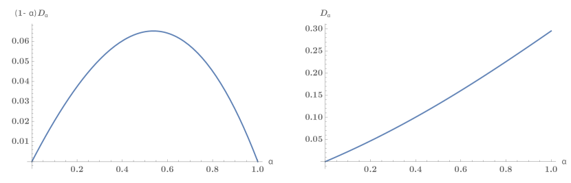
Figure 5: Renyi divergence (118) for the sine-squared deformation with $L=1,c=30,\beta=0.1,g=0.04$.

5.3 Higher spin generalisation

We can also consider inhomogneous deformation by higher spin currents

$$\delta H_{s}=\int_{0}^{L}dx~{}\left[\frac{g}{2^{k}}\left(e^{-{2\pi x\over L}(s-2+k)}+e^{-{2\pi x\over L}(s-2-k)}\right)\right]~{}V^{(s)}_{00...}(x)$$ (120)

Here, $V^{(s)}$ denotes a higher spin current with spin $s$. In the previous section the case with $s=2$ and $k=1$ was considered. Recall that, in terms of modes

$$V^{(s)}(z)=\sum_{n=-\infty}^{\infty}\frac{V^{(s)}_{n}}{z^{n+s}}~{}.$$ (121)

The deformation is then

$$\delta H_{s}=\frac{2\pi}{L}\frac{g}{2^{k}}\int_{C}\frac{dz}{2\pi i}\left[z^{s-1+k}+{z^{s-1-k}}\right]V^{(s)}(z)=\frac{2\pi}{L}\frac{g}{2^{k}}[V^{(s)}_{-k}+V^{(s)}_{k}]~{}.$$ (122)

The deformation by the spin-3 current turns out to be simpler than other ones. The torus partition function can be exactly found just like the Möbius deformation, it leads to effective rescaling of the modular parameter. For the deformation by $W_{-2}+W_{2}$ we have

$$\mathcal{Z}_{g}(\tau,\bar{\tau}) =\text{Tr}\left[q^{L_{0}+\frac{g}{4}(W_{-2}+W_{2})-c/24}\bar{q}^{\bar{L}_{0}+\frac{g}{4}(\bar{W}_{-2}+\bar{W}_{2})-c/24}\right]$$

$$=(q\bar{q})^{-(1-\sqrt{1+4g^{2}}){c\over 24}}\mathcal{Z}_{\rm CFT}(\tau\sqrt{1+4g^{2}},\bar{\tau}\sqrt{1+4g^{2}})~{}.$$ (123)

The details of this calculation can be found in Appendix B.2.

Renyi divergence

Once again we are interested in the trace with two Boltzmann factor insertions

$$\mathcal{Z}_{g}(\tau,\bar{\tau}|\alpha) =\text{Tr}\left[q^{\alpha(L_{0}+\frac{g}{2^{k}}(V^{(s)}_{-k}+V^{(s)}_{k})-{c\over 24})}\bar{q}^{\alpha(\bar{L}_{0}+\frac{g}{2^{k}}(\bar{V}^{(s)}_{-k}+\bar{V}^{(s)}_{k})-{c\over 24})}q^{(1-\alpha)(L_{0}-{c\over 24})}{\bar{q}}^{(1-\alpha)(\bar{L}_{0}-{c\over 24})}\right].$$ (124)

We restrict $k$ to $1<|k|<s$ so that the corrections are determined by the global hs$[\lambda]$ algebra. For calculating the corrections perturbatively, the steps till (111) are the same – we just need to replace the deforming operator appropriately. The second order correction is (writing just the holomorphic piece for the time being and $b=-\log q$ as before)

$$\frac{\partial^{2}\mathcal{Z}_{\rm hol}}{\partial g^{2}}\bigg{|}_{g=0}=~{} \frac{(\alpha b)^{2}}{2^{2k-1}}\int_{0}^{1}ds~{}(1-s)\int_{0}^{1}du~{}\text{Tr}\left[e^{-b(1-\alpha u(1-s))L_{0}}V^{(s)}_{+}e^{-\alpha b(1-s)uL_{0}}V^{(s)}_{+}\right],$$

where, $V^{(s)}_{+}=V^{(s)}_{k}+V^{(s)}_{-k}$. The higher spin currents can be shuffled using the following identity

$$\text{Tr}\left[(V^{(s)}_{k}+V^{(s)}_{-k})y^{L_{0}}(V^{(s)}_{k}+V^{(s)}_{-k})w^{L_{0}}\right] =(y^{k}+w^{k})\,\text{Tr}\left[V^{(s)}_{k}V^{(s)}_{-k}q^{L_{0}}\right].$$ (126)

This is proved in the Appendix C. The trace appearing above can be calculated in the same manner as the Virasoro case – see equation (C.1). The final result for the second order correction is

$$\frac{\partial^{2}\mathcal{Z}_{g}}{\partial g^{2}}\bigg{|}_{g=0}= -\tfrac{2^{1-2k}q^{k}}{k}\tfrac{4q^{k/2}\sin(\pi(\alpha-1)k\tau)\sin(\pi\alpha k\tau)+k\alpha(1-q^{k})\log q}{1-q^{k}}~{}{(q{\bar{q}})^{-c/24}}C^{2}_{ss}(k,\lambda)~{}\partial_{q}f(\tau,\bar{\tau})+\cdots$$

$$+\text{anti-holomorphic}~{}.$$ (127)

Here, $C_{NN}^{2}(k,\lambda)$ is the following structure constant appearing in the hs$[\lambda]$ algebra (see e.g. (Gaberdiel:2011wb, , Appendix A))

$$[V^{(s)}_{-k},V^{(s)}_{k}]=C_{ss}^{2}(k,\lambda)L_{0}+\text{zero-modes of even spins}.$$ (128)

Equation (5.3) reduces to the Möbius deformation for $s=2$ and $k=1$ given in equation (5.2). It also reduces to perturbatively expanded $\mathcal{W}_{3}$ result (5.3) for $\alpha=1$, $\lambda=-3$, $s=3$ and $k=2$. The ‘$\cdots$’ in (5.3) involve expectation values of even-spin currents. These vanish in the high temperature limit if we choose to work in the primary basis.

The partition function (124) is then

$$\mathcal{Z}_{g}(\tau,\bar{\tau}|\alpha)=~{}\mathcal{Z}_{\rm CFT}(\tau,\bar{\tau})$$

$$-g^{2}\left[\tfrac{2^{-2k}q^{k}}{k}\tfrac{4q^{k/2}\sin(\pi(\alpha-1)k\tau)\sin(\pi\alpha k\tau)+k\alpha(1-q^{k})\log q}{1-q^{k}}~{}{(q{\bar{q}})^{-c/24}}C^{2}_{ss}(k,\lambda)~{}\partial_{q}f(\tau,\bar{\tau})+\text{anti-hol}\right]$$

$$+O(g^{3})~{}.$$ (129)

Here we have not written terms arising from even-spin currents. As before, the Renyi divergence can be found straightforwardly from the above deformed partition function. The leading order result is

$$D_{\alpha}(\rho_{g}||\rho_{\beta})\approx-g^{2}\bigg{[} \frac{2^{-2k}q^{k}}{k}\frac{4q^{k/2}\sin(\pi(\alpha-1)k\tau)\sin(\pi\alpha k\tau)}{(1-q^{k})(1-\alpha)}~{}C^{2}_{ss}(k,\lambda)~{}\partial_{q}{\log}f(\tau,\bar{\tau})$$

$$+\text{anti-holomorphic}\bigg{]}.$$ (130)

We note that this result takes a universal form for all higher-spin inhomogeneous deformations considered here. The dependence on the spin of the deforming current appears only through the structure constant $C_{ss}^{2}$.

We can also consider the deformation of the CFT Hamiltonian by the operator $J_{1}+J_{-1}$ built from the modes of $U(1)$ current. The Rényi divergence can be analogously computed and we have the leading result

$$D_{\alpha}(\rho_{g}||\rho_{\beta})\approx g^{2}\bigg{[} \frac{q^{3/2}\sin(\pi(\alpha-1)\tau)\sin(\pi\alpha\tau)}{(1-q)(1-\alpha)}~{}\kappa+\text{anti-holomorphic}\bigg{]},$$ (131)

where, $\kappa$ is the level of the current algebra.

The $\alpha$ dependence in the leading correction for the inhomogeneous deformations considered here takes exactly the same form as the deformed harmonic oscillator (96). The frequency $\omega$ of the harmonic oscillator gets replaced by the mode number $k$. Note that the $\alpha$ dependence is fixed by the same integral which appears in (5.2), (5.3) and (C.2). The integrand is, in turn, determined by the following commutators with the undeformed Hamiltonians

$$[H_{\rm CFT},L_{k}]=-kL_{k},\qquad[H_{\rm CFT},V^{(s)}_{k}]=-kV^{(s)}_{k},\qquad[H_{\rm SHO},a_{\pm}]=\pm\omega a_{\pm},$$ (132)

where, we set the length of the spatial circle $L=2\pi$ and $\hbar=1$. In particular, these relations facilitate rearrangement of operators within the traces and Boltzmann factors (see Appendix C). The similar form of these algebraic relations is the reason behind the universality at the leading order.

6 Generalized second laws of thermodynamics

One of the aims of Bernamonti:2018vmw to study Rényi divergences in conformal field theories was the possibility that they provide additional constraints on thermodynamical evolution for out of equilibrium systems besides the ordinary second law. These constraints are a natural extrapolation of the simple thermodynamical criterion that a transition from the state $\rho_{1}$ to $\rho_{2}$ is allowed provided the free energy $F(\rho_{1})>F(\rho_{2})$. Note that we are considering open systems, and each of these density matrices are in contact with its respective heat baths. We have seen in equation (13), that one of the properties of the Rényi divergence $D_{\alpha}(\rho||\rho_{\beta})$ is that at $\alpha=1$, it reduces to the differences between the free energies of the density matrices $\rho$ and $\rho_{\beta}$. Using this property we can arrive at the following equivalent statement of the second law. Consider the difference

$$\delta D_{1}(\rho_{1}||\rho_{2})\equiv D_{1}(\rho_{1}||\rho_{\beta})-D_{1}(\rho_{2}||\rho_{\beta}).$$ (133)

Then if $\delta D_{1}(\rho_{1}||\rho_{2})>0$, the occurrence of the state $\rho_{2}$ in a transition from $\rho_{1}$ to $\rho_{\beta}$ is allowed by the conventional second law. The generalized 2nd law is the statement that state $\rho_{2}$ is allowed in a transition from $\rho_{1}$ to $\rho_{\beta}$ only if Brand_o_2015 ; Bernamonti:2018vmw

$$\delta D_{\alpha}(\rho_{1}||\rho_{2})\equiv D_{\alpha}(\rho_{1}||\rho_{\beta})-D_{\alpha}(\rho_{2}||\rho_{\beta})>0,\qquad{\mbox{for all }}\alpha.$$ (134)

A heuristic understanding of this generalization can be obtained by considering the microcanonical ensemble. This implies $\rho_{\beta}\rightarrow\rho^{*}$ where $\rho^{*}$ is the equal a-priori probability distribution. The above statement is then equivalent to maximizing the Rényi entropy during a transition.

Thus, the generalized second laws in principle represent more constraints that the traditional second law. However, it need not be always the case. Consider a plot of of $\delta D_{\alpha}(\rho_{1}||\rho_{2})$ as shown in the figure 6(a). It is clear from the shape of the graph that the transition from $\rho_{1}$ to $\rho_{2}$ which is allowed by the traditional second law at $\alpha=1$ continues to be allowed for all $0<\alpha<1$. In this situation, the generalized second law does not provide any further constraint than that by the conventional second law. However if the shape of the graph is as shown in figure 6(b), then the generalized state that the transition $\rho_{1}$ to $\rho_{2}$ which is allowed by the conventional second law at $\alpha=1$ is forbidden by the generalized second law. It is important that this discussion is for open systems in contact with the heat bath and not for closed system where we also need to ensure conservation of energy.

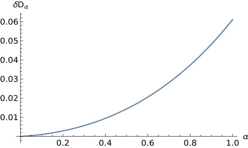
(a)

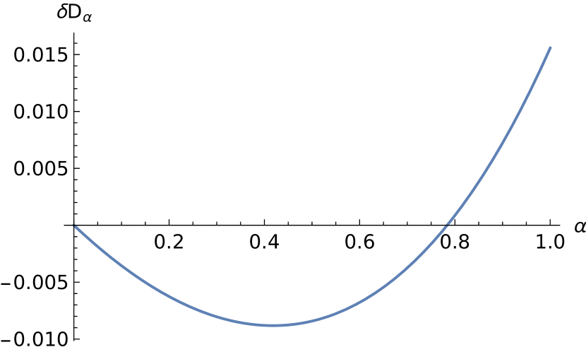
(b)

Figure 6: (Left) A sample plot of $\delta D_{\alpha}(\rho_{1}||\rho_{2})$ showing the case where there are no additional constraints from the generalized second law for the transition from $\rho_{1}\rightarrow\rho_{2}$. (Right) A sample plot of $\delta D_{\alpha}(\rho_{1}||\rho_{2})$ showing that the generalized second law disallows the transition from $\rho_{1}\rightarrow\rho_{2}$ even though it is allowed by the conventional second law.

In this section we will use the results for Rényi divergences of sections and obtain situations of the kind shown in figure 6(b). We will see in all the case we study there are situations in which the generalised second laws do indeed represent additional constraints. This study extends the observations of Bernamonti:2018vmw which were made for excitations $\rho_{1},\rho_{2}$ corresponding to deformations by conformal primaries of weights $\Delta_{1},\Delta_{2}$ respectively.

6.1 Higher temperature to spin-1 charged states

Let us consider the case of of the Rényi divergence of excited state corresponding to the stress temperature deformation, $\rho_{T}$ and that of the $U(1)$ current deformation $\rho_{J}$. From (58) and (75), we write these results as

$$D_{\alpha,J}(\rho_{J}||\rho_{\beta}) = \frac{\pi cL}{6\beta}\mu_{J}^{2}\alpha,$$ (135)

$$D_{\alpha,T}(\rho_{T}||\rho_{\beta}) = \frac{\pi cL}{6\beta}\left(\frac{\mu_{T}^{2}\alpha}{(1-\mu_{T})(1-\alpha\mu_{T})}\right).$$

Here the $U(1)$ deformation has been redefined as

$$2\pi\kappa\mu^{2}\beta^{2}\rightarrow\mu^{2}_{J}~{},$$ (136)

and the stress tensor deformation is defined as

$$2\pi\mu\rightarrow\mu_{T}~{}.$$ (137)

With these definitions both $\mu_{J},\mu_{T}$ are dimensionless, $\rho_{\beta}$ is the reference thermal state. Note that the excited state corresponding to the stress tensor deformation can be thought of a thermal state at temperature

$$T^{\prime}=\frac{T}{1-\mu_{T}}~{}.$$ (138)

Let us define the difference of the Rényi divergences which is given by

$$\delta D_{\alpha}(\rho_{T}||\rho_{J})=\frac{\pi cL}{6\beta}\left(\frac{\mu_{T}^{2}\alpha}{(1-\mu_{T})(1-\alpha\mu_{T})}-\mu_{J}^{2}\alpha\right)~{}.$$ (139)

In the figure 7(a) we have the Rényi divergences for $\mu_{T}=0.3$ along with various values of $\mu_{J}$. It can be seen that $\mu_{J}=0.42,0.38$, that the excited state $\rho_{J}$ is allowed by the traditional second law but disallowed by the generalized second law. This is also clear from the plot of $\delta D_{\alpha}(\rho_{T}||\rho_{J})$ in figure 7(b). Note that for $\mu_{J}=0.46$, the charged state is prevented to occur as an intermediate state even by the second law.

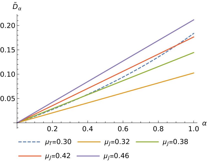
(a)

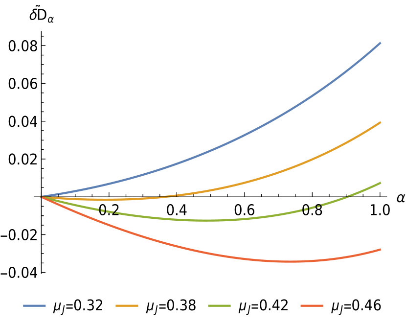
(b)

Figure 7: (Left) $\tilde{D}_{\alpha}=\frac{6\beta}{\pi cL}D_{\alpha}$ vs $\alpha$ for fixed $\mu_{T}=0.3$. Values of $\mu_{J}$ decrease on the curves from top to bottom. (Right) plot of $\delta\tilde{D}_{\alpha}=\frac{6\beta}{\pi cL}\delta D_{\alpha}(\rho_{T}||\rho_{J})$ vs $\alpha$ for fixed $\mu_{T}=0.3$. Note the transition represented by the curves $\mu_{J}=0.42,0.38$ are allowed by the conventional first law but disallowed by the generalised second laws of thermodynamics.

Since we have analytical expressions for the Rényi divergences, it is easy to find the domains for which the intermediate state $\rho_{J}$ is allowed to occur by the generalized second law for transitions from higher temperature to lower temperature. Therefore form (138) we have $0<\mu_{T}<1$ and without loss of generality we can chose $\mu_{J}$ to be positive.

• For small enough chemical potentials given by

  $$\mu_{J}<\frac{\mu_{T}}{\sqrt{1-\mu_{T}}}=\frac{T^{\prime}-T}{\sqrt{TT^{\prime}}},\qquad D_{\alpha,J}(\rho_{J}||\rho_{\beta})<D_{\alpha,T}(\rho_{T}||\rho_{\beta}),$$ (140)

  we see that the charged excited state $\rho_{J}$ is allowed by the both the conventional second law and the generalised second law.

• For chemical potentials in the range

  $$\frac{\mu_{T}}{\sqrt{1-\mu_{T}}}<\mu_{J}<\frac{\mu_{T}}{1-\mu_{T}}=\frac{T^{\prime}-T}{T},$$ (141)

  the excited state $\rho_{J}$ is allowed by the conventional second law, but disallowed by the generalised second law. Note that for this range we have $\delta D_{1}(\rho_{T}||\rho_{J})>0$.

• For large chemical potentials in the range

  $$\frac{\mu_{T}}{1-\mu_{T}}<\mu_{J},\qquad D_{\alpha,T}(\rho_{T}||\rho_{\beta})<D_{\alpha,J}(\rho_{J}||\rho_{\beta}),$$ (142)

  the transition intermediate state $\rho_{J}$ does not occur in the transition from $\rho_{T}$ to $\rho_{\beta}$.

6.2 Transitions between two temperatures

We have seen that given the stress tensor deformation $\mu_{1}$, the density matrix of the excited state corresponds to that of temperature

$$T_{1}=\frac{T}{1-\mu_{1}}.$$ (143)

The Rényi divergence is given by

$$D_{\alpha}(\rho_{1}||\rho_{\beta})=\frac{\pi cL}{6\beta}\left(\frac{\mu_{1}^{2}\alpha}{(1-\mu_{1})(1-\mu_{1}\alpha)}\right).$$ (144)

Transitions from higher temperature to lower temperature

Let the state $\rho_{1}$ be at higher temperature, $0<\mu_{1}<1$ . Now consider another state $\rho_{2}$ corresponding to the stress tensor deformation $\mu_{2}$. We can now ask in the transition from $\rho_{1}$ to $\rho_{\beta}$ is it possible that the state $\rho_{2}$ be allowed by the traditional second law, but dis-allowed by the generalised second law. In figure 8(a) we have plotted various values of $\mu_{2}$ for a fixed value of $\mu_{1}=0.3$. We find that for $-0.75<\mu_{2}<-0.428$, that is a band of lower temperatures than $T$, it is indeed the case that there are situations where the traditional first law at $\alpha=1$ allows the state $\rho_{2}$ to occur in the transition from $\rho_{1}\rightarrow\rho_{\beta}$, however the generalised second law prohibits this process. This is also confirmed in figure 8(b) which plots the difference in Rényi divergences defined by

$$\delta_{\alpha}D_{\alpha}(\rho_{1}||\rho_{2})=\frac{\pi cL}{6\beta}\left(\frac{\mu_{1}^{2}\alpha}{1-\mu_{1})(1-\mu_{1}\alpha)}-\frac{\mu_{2}^{2}\alpha}{(1-\mu_{2})(1-\mu_{2}\alpha)}\right)~{}.$$ (145)

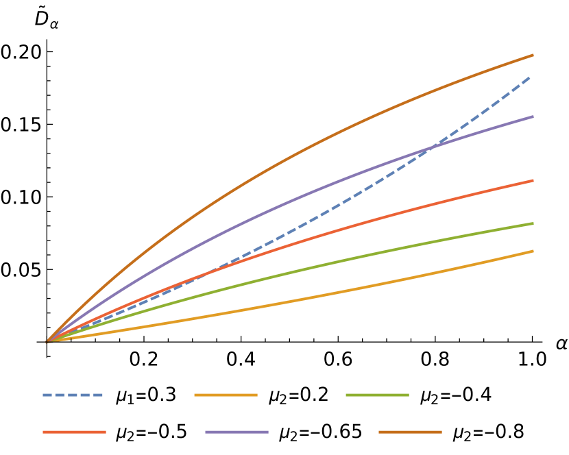
(a)

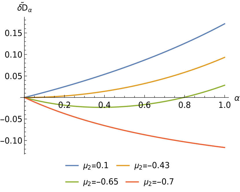
(b)

Figure 8: (Left) $\tilde{D}_{\alpha}=\frac{6\beta}{\pi cL}D_{\alpha}$ vs $\alpha$ for fixed $\mu_{1}=0.3$, we see the the generalised second law prevents transitions to states with $\mu_{2}$ in the range $\frac{\mu_{1}}{2\mu_{1}-1}=-0.75<\mu_{2}<\frac{\mu_{1}}{\mu_{1}-1}=-0.428$. The conventional second law disallows states with $\mu_{2}<-0.75$. (Right) $\delta\tilde{D}_{\alpha}=\frac{6\beta}{\pi cL}\delta D_{\alpha}(\rho_{1}||\rho_{2})$ vs $\alpha$ for fixed $\mu_{1}=0.3$ and different $\mu_{2}$.

Since we have analytical and simple algebraic expressions for the Rényi divergences, by studying various inequalities we can make the following general statements for the transition form $(\rho_{1},\mu_{1})$ at higher temperature to $\rho_{\beta}$.

• In the range $\frac{1}{2}\leq\mu_{1}<1$, we see that for $\mu_{2}<\mu_{1}$ and for $0<\alpha<1$ we have

  $$D_{\alpha}(\rho_{1}||\rho_{2})>0\quad{\rm for}\;\;\frac{1}{2}<\mu_{1}<1\quad{\rm and}\;\;\mu_{2}<\mu_{1}~{}.$$ (146)

  This of course implies that there are no situations in which the generalised second law implies more constraints than the conventional second law.

• In the range $0<\mu_{1}<\frac{1}{2}$, for states with

  $$D_{\alpha}(\rho_{1}||\rho_{2})>0\quad{\rm for}\;\;0<\mu_{1}<\frac{1}{2}\quad{\rm and}\;\;-\frac{\mu_{1}}{1-\mu_{1}}<\mu_{2}<\mu_{1}~{}.$$ (147)

  Again this implies that there are no situations in which the generalised second law implies more constraints than the conventional second law.

• But in the range

  $$0<\mu_{1}<\frac{1}{2}\quad{\rm and}\;\;-\frac{\mu_{1}}{1-2\mu_{1}}<\mu_{2}<-\frac{\mu_{1}}{1-\mu_{1}},$$ (148)

  we see that the generalised second law prevents the occurrence of the state $(\rho_{2},\mu_{2})$ in the transition from $(\rho_{1},\mu_{1})$ to $\rho_{\beta}$ which is allowed by the traditional second law.

• Finally in the range

  $$0<\mu_{1}<\frac{1}{2}\quad{\rm and}\;\;-\infty<\mu_{2}<-\frac{\mu_{1}}{1-2\mu_{1}}.$$ (149)

  The traditional second law itself prevents the occurrence of the state $(\rho_{2},\mu_{2})$ .

In summary we conclude that in a transition from as state of higher temperature $(\rho_{1},\mu_{1})$ to $\rho_{\beta}$, the states which are allowed to occur by the generalised second law satisfies the condition,

$$-\frac{\mu_{1}}{1-\mu_{1}}<\mu_{2}<\mu_{1}.$$ (150)

It is interesting to note that $T_{1}=\frac{T}{1-\mu_{1}}$ the lowest temperature $T_{2}^{*}=-\frac{\mu_{1}}{1-\mu_{1}}$ allowed satisfies the following property

$$T_{1}T_{2}^{*}=T.$$ (151)

That is $T$ is the geometric mean of $T_{1}$ and $T_{2}^{*}$.

Transitions from lower temperature to higher temperature

In the transition from the excited state $\rho_{1}$ with $-\infty<\mu_{1}<0$ to $\rho_{\beta}$ we find that there are no situations in which the generalized second law prevents a transition which is allowed by the traditional second law. The higher temperature states $(\rho_{2},\mu_{2})$ which are allowed as intermediate states in this transition satisfy the condition

$$-\infty<\mu_{1}<0\quad{\rm and}\;\;\;\mu_{1}<\mu_{2}<\frac{-\mu_{1}}{1-2\mu_{1}}.$$ (152)

It is again interesting to note that $T_{1}=\frac{T}{1-\mu_{1}}$ and highest temperature $T_{2}^{*}=\frac{-\mu_{1}}{1-2\mu_{1}}$ which is allowed satisfies the property

$${T_{1}+T_{2}^{*}}=2T.$$ (153)

Here $T$ is the arithmetic mean of $T_{1}$ and $T_{2}^{*}$.

6.3 Spin-3 charged state to higher temperature

Let us consider transitions from the excited state corresponding to the spin-3 deformation $(\rho_{W},\mu_{W})$ to the state $(\rho_{T},\mu_{T})$ which is the excited state corresponding to the stress tensor deformation. From (4.3) and (75) the Rényi divergences for these states are given by

$$D_{\alpha}(\rho_{W}||\rho_{\beta}) = \frac{\pi cL}{6\beta}\left[\frac{16}{3}\left(\frac{\pi\mu_{W}}{\beta}\right)^{2}\alpha+\frac{12800}{27}\left(\frac{\pi\mu_{W}}{\beta}\right)^{4}\alpha(\alpha^{2}+\alpha+1)+\cdots\right],$$

$$D_{\alpha,T}(\rho_{T}||\rho_{\beta}) = \frac{\pi cL}{6\beta}\left(\frac{\mu_{T}^{2}\alpha}{(1-\mu_{T})(1-\alpha\mu_{T})}\right)$$ (154)

Let us also define

$$\delta D_{\alpha}(\rho_{W}||\rho_{T})=D_{\alpha}(\rho_{W}||\rho_{\beta})-D_{\alpha,T}(\rho_{T}||\rho_{\beta})~{}.$$ (155)

We can study if there are additional constraints from the generalised second law for the occurrence of the state $(\rho_{T},\mu_{T})$ in the transition from $(\rho_{W}||\rho_{\beta})$ to $\rho_{\beta}$. The series representing $D_{\alpha}(\rho_{W}||\rho_{\beta})$ is an asymptotic series for small $\mu_{W}$. Therefore to trust our results we need to take the values of $\mu_{W}$ and the number of terms in the expansion with care. In figure 9 we have plotted $\delta D_{\alpha}(\rho_{W}||\rho_{T})$ for a fixed $\mu_{W}=0.002$ for three values of $\mu_{T}$. We have kept to order $\mu_{W}^{20}$ terms in the expansion of $D_{\alpha}(\rho_{W}||\rho_{\beta})$, and have verified that the asymptotic expansion gives the same curves by keeping terms to order $\mu_{W}^{10}$ or to order $\mu_{W}^{50}$. Thus the asymptotic expansion gives stable values for $\delta D_{\alpha}(\rho_{W}||\rho_{T})$ for $\mu_{W}=0.002$. Note that the curve for $\mu_{T}=0.022875$ represents the situation for which the state $\rho_{T}$ is allowed for the transition from $\rho_{W}$ to $\rho_{\beta}$ by the conventional second law of thermodynamics but is disallowed by the generalized second laws. We have also seen, that there are such additional constraints from the generalized second laws for the occurrence of $\rho_{W}$ in transitions from the state at higher temperature to the charged spin-3 state $\rho_{W}$.

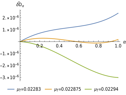
Figure 9: $\tilde{D}_{\alpha}=\left(\frac{6\beta}{\pi cL}\right)\delta D_{\alpha}(\rho_{W}||\rho_{T})$ vs $\alpha$ for fixed $\mu_{W}=0.02$. The transition represented by the curve for $\mu_{T}=0.022875$ is allowed by the conventional second law but disallowed by the generalized second laws of thermodynamics.

6.4 Transitions involving SSD states

The Rényi divergences of the excited state $(\rho_{k=1}$ corresponding to the SSD deformation $g(L_{1}+L_{-1})$ in the Hamiltonian to the quadratic order in perturbation theory on the torus is given by

$$D_{\alpha}(\rho_{k=1}||\rho_{\beta}) = \mu_{1}^{2}\frac{\pi cL}{6\beta}\frac{\sinh\frac{\pi\alpha\beta}{L}\sinh\frac{\pi(\alpha-1)\beta}{L}}{\alpha-1}.$$ (156)

Here we have taken a rectangular torus by setting $\tau=\frac{i\beta}{L}$ and absorbed the prefactors $2g^{2}q\partial_{q}\log f(\tau,\bar{\tau})$ into the coupling $\mu_{1}$. This is possible since we work at a fixed $\tau$. We can now consider transitions between the SSD deformed state $(\rho_{k=1},\mu_{1})$ and the excited state corresponding to the stress tensor deformation $(\rho_{T},\mu_{T})$ with Rényi divergence

$$D_{\alpha}(\rho_{T}||\rho_{\beta}) = \frac{\pi cL}{6\beta}\left(\frac{\mu_{T}^{2}\alpha}{(1-\mu_{T})(1-\alpha)}\right).$$ (157)

Let us define the difference

$$\delta D_{\alpha}(\rho_{k=1}||\rho_{T})=D_{\alpha}(\rho_{k=1}||\rho_{\beta})-D_{\alpha}(\rho_{T}||\rho_{\beta}).$$ (158)

In figure 10(a) we have plotted the Rényi divergences of the excited states corresponding to the $(\rho_{T},\mu_{T})$ for different values of $\mu_{T}$ along with the Rényi divergence of the SSD state $(\rho_{T},\mu_{1})$ at $\mu_{1}=0.05$. We see that for $\mu_{T}=0.22$, the transition from the SSD excited state is allowed by the conventional second law, but disallowed by the generalised second laws. This can also be seen in figure 10(b) which plots the difference $\delta D_{\alpha}(\rho_{k=1}||\rho_{T})$. We have chosen value of $\beta/L=1$ and $\mu_{1}$ so that it

$$\mu_{1}^{2}\ll\frac{1}{\pi\sinh\pi}$$ (159)

This ensures that the Rényi divergence at $\alpha=1$, its largest value is small so that perturbation theory can be trusted.

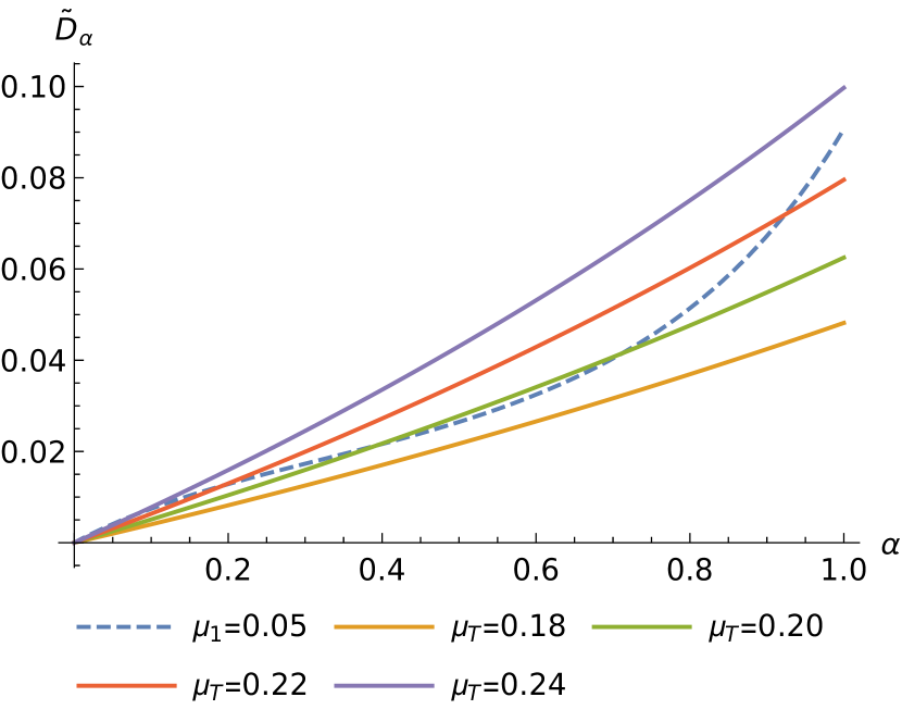
(a)

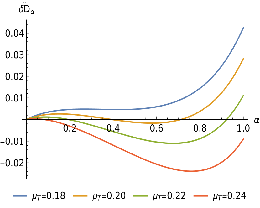
(b)

Figure 10: (Right) $\tilde{D}_{\alpha}=\frac{6\beta}{\pi cL}D_{\alpha}$ vs $\alpha$ for different values of $\mu_{T}$ and fixed $\mu_{1}=0.05$. (Left) $\delta\tilde{D}_{\alpha}=\delta D_{\alpha}(\rho_{k=1}||\rho_{T})$ for a fixed $\mu_{1}=0.05$. We have set $\beta/L=1$ The transition represented by the curve $\mu_{T}=0.22$ is allowed by the conventional second law but disallowed by the generalized second laws.

Finally let us consider transitions from the SSD state $(\rho_{k=2},\mu_{2})$ with Rényi divergence given by. Here the SSD state is obtained by adding the deformation $g(V_{2}^{(s)}+V_{-2}^{(s)})$.

$$D_{\alpha}(\rho_{k=2}||\rho_{\beta})=\mu_{2}^{2}\frac{\pi cL}{6\beta}\frac{\sinh\frac{2\pi\alpha\beta}{L}\sinh\frac{2\pi(\alpha-1)\beta}{L}}{\alpha-1}$$ (160)

To obtain this expression we have taken $\tau=\frac{i\beta}{L}$ in (5.3) and absorbed all the resulting prefactors into $\mu_{2}^{2}$. We can also consider the difference

$$\delta D_{\alpha}(\rho_{k=2}||\rho_{k=1})=\mu_{1}^{2}\frac{\pi cL}{c\beta}\left(\frac{\gamma\sinh\frac{2\pi\alpha\beta}{L}\sinh\frac{2\pi(\alpha-1)\beta}{L}}{\alpha-1}-\frac{\sinh\frac{\pi\alpha\beta}{L}\sinh\frac{\pi(\alpha-1)\beta}{L}}{\alpha-1}\right),$$

where the ratio $\gamma=(\frac{\mu_{2}}{\mu_{1}})^{2}$.

In figure 11(a), we have plotted the Rényi divergences of excited state $(\rho_{k=2},\mu_{2})$, $(\rho_{k=1},\mu_{1})$ for various values of the ratio $\gamma$. The Rényi divergences are normalized by dividing $\frac{\pi cL\mu_{1}^{2}}{6\beta}$. The dashed curve represents the SSD deformation for $k=1$, while the solid curves are that for $k=2$. The curves corresponding to $\gamma=0.035,0.025$ are transitions from the $k=2$ SSD excited state to the $k=1$ SSD state which is allowed by the conventional second law, but prohibited by generalised second laws. We have set $\frac{\beta}{L}=1$. Figure 11(b), show the same by plotting $\delta D_{\alpha}(\rho_{k=2}||\rho_{k=1})$ for various values of $\gamma$.

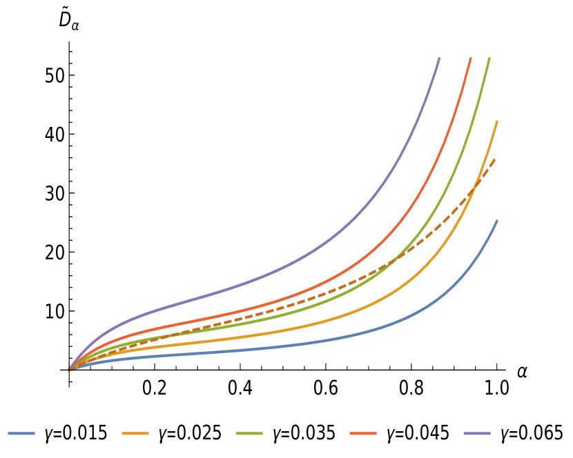
(a)

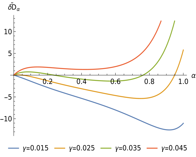
(b)

Figure 11: (Left) $\tilde{D}_{\alpha}=\left(\frac{6\beta}{\pi cL\mu_{1}^{2}}\right)D_{\alpha}$ with $\frac{\beta}{L}=1$.The dashed curve represents $\frac{6\beta}{\pi cL\mu_{1}^{2}}D_{\alpha}(\rho_{k=1}||\rho_{\beta})$. The coloured curves correspond to $\frac{6\beta}{\pi cL\mu_{1}^{2}}D_{\alpha}(\rho_{k=1}||\rho_{\beta})$ for different values of $\gamma$. The curves $\gamma=0.035,0.025$ represent a transition from the SSD $k=2$ excited state to the $k=1$ state which is allowed by the second law but prohibited by the generalised second law. (Right) $\delta\tilde{D}_{\alpha}=\left(\frac{6\beta}{\pi cL\mu_{1}^{2}}\right)\delta D_{\alpha}(\rho_{2}||\rho_{1})$ for various values of $\gamma$.

7 Conclusions

In this paper we evaluated the Rényi divergences between the thermal density matrix and excited states created by deforming the Hamiltonian by scalar primaries, conserved currents and SSD deformations in 2d CFTs. One of our aims was to obtain tractable examples so that the properties of Rényi divergences can be studied further. Our study has shown that the $\alpha$ dependence of leading correction to the Rényi divergences is universal as long as the deforming operators together with the Hamiltonian satisfy the Heisenberg algebra. Indeed as far as we are aware, the $\alpha$ dependence of Rényi divergences have been obtained only numerically as in Bernamonti:2018vmw . Systems such as the ones considered in this paper with simple $\alpha$ dependence for which Rényi divergences can be obtained exactly have not been studied. We used these simple examples to show that the generalized second laws of thermodynamics put forward in Brand_o_2015 ; Bernamonti:2018vmw do place more constraints on the evolution of non-equilibrium systems compared to the traditional second law. The methods developed in this paper – conformal perturbation theory for holomorphic deformations and Hamiltonian perturbation theory – can be used for other systems.

It is worthwhile to consider Rényi divergences beyond the ones considered in this work and Bernamonti:2018vmw . Specifically, an interesting future problem is to study the Rényi divergence for the $T\bar{T}$ deformation Cavaglia:2016oda ; Smirnov:2016lqw . This entails the calculation of

$$\mathcal{Z}_{\alpha}(\lambda)=\text{Tr}[q^{\alpha H_{T\bar{T}}(\lambda)}q^{(1-\alpha)H_{\rm CFT}}]~{},$$

where, $\lambda$ is the $T\bar{T}$ coupling. Analysing this quantity would shed light on the differences in the nature of eigenstates of the deformed and undeformed theories. Note that although the spectrum of $H_{T\bar{T}}$ and $H_{\rm CFT}$ are related by a one-to-one map, the Hamiltonians themselves do not commute. This renders the calculation of $\mathcal{Z}_{\alpha}(\lambda)$ non-trivial. One way to proceed is to derive a flow equation for the above quantity along the lines of Cardy:ttb or potentially bootstrapping using modular properties Aharony:2018bad ; Datta:2018thy . Moreover, it would also be fruitful to check whether the integration prescription used in this work or variants discussed in Datta:2014zpa can be employed to treat this deformation perturbatively.

Finally, the universality in the $\alpha$ dependence of Rényi divergences for SSD deformations encourages us that it is worthwhile to engineer holographic setups for such quenches. The SL$(2,\mathbb{R})$ Chern-Simons theory in 3-dimensions and its higher spin generalization provide natural frameworks to think of these deformations. This will not only teach us more about holography in these systems, but also lead to constructions with Euclidean time dependences in the bulk. Such aspects of holography have not been fully explored. It will be interesting to see whether such holographic setups together with the generalised second laws will have lessons for the processes of black hole formation and evaporation.

Appendix A Details for spin-2 and spin-3 deformations

In this appendix we provide the details of the correlations functions and the integrals for evaluating the partitions functions for spin-2 and spin-3 deformations. For these deformations we carry out the perturbative expansion to order $\mu^{4}$.

A.1 Spin-2 deformation to the quartic order

To carry out the the perturbative expansion of the partition function in (4.2) to order $\mu^{4}$ we would require the $3$ point function and the $4$ point function of the stress tensor on the cylinder as well as the integrals on the cylinder.

We begin with the $3$-point function of the stress tensor on the plane, which is given by

$$\langle T(\omega_{1})T(\omega_{2})T(\omega_{3})\rangle=\left(\frac{\pi}{\beta}\right)^{6}\frac{c}{\sinh^{2}\frac{\pi}{\beta}(w_{1}-w_{2})\sinh^{2}\frac{\pi}{\beta}(w_{2}-w_{3})\sinh^{2}\frac{\pi}{\beta}(w_{1}-w_{3})}$$

$$\qquad\qquad-\frac{c^{2}}{12}\left(\frac{\pi}{\beta}\right)^{6}\left(\frac{1}{\sinh^{4}\frac{\pi}{\beta}(w_{1}-w_{2})}+\frac{1}{\sinh^{4}\frac{\pi}{\beta}(w_{2}-w_{3})}+\frac{1}{\sinh^{4}\frac{\pi}{\beta}(w_{1}-w_{3})}\right)$$

$$\qquad\qquad-\frac{c^{3}\pi^{6}}{216\beta^{6}}~{}.$$ (162)

We now integrate the $3$-point function on the cylinder using the prescription discussed in section 4. This results in

$$\int d^{2}\omega_{1}\int d^{2}\omega_{2}\int d^{2}\omega_{3}\langle T(\omega_{1})T(\omega_{2})T(\omega_{2})\rangle=-\frac{4cL\pi^{4}}{\beta}-\frac{c^{2}L^{2}\pi^{5}}{3\beta^{2}}-\frac{c^{3}L^{3}\pi^{6}}{216\beta^{3}}.$$

The $4$-point function of the stress tensor on the cylinder can be obtained using the conformal Ward identity. It is given by

$$\langle T(\omega_{1})T(\omega_{2})T(\omega_{3})T(\omega_{4})\rangle=\langle T(\omega_{1})T(\omega_{2})T(\omega_{3})T(\omega_{4})\rangle^{(0)}=$$ (164)

$$-\frac{c^{2}}{6}\left(\frac{\pi}{\beta}\right)^{8}\left(\frac{1}{\sinh^{2}\frac{\pi}{\beta}(w_{1}-w_{2})\sinh^{2}\frac{\pi}{\beta}(w_{2}-w_{3})\sinh^{2}\frac{\pi}{\beta}(w_{1}-w_{3})}+3\;{\rm permutations}\right)$$

$$\qquad\qquad\qquad\qquad\qquad+\frac{c^{3}}{72}\left(\frac{\pi}{\beta}\right)^{8}\left(\frac{1}{\sinh^{2}\frac{\pi}{\beta}(w_{1}-w_{2})}+5\;{\rm permutations}\right)$$

$$\qquad\qquad\qquad\qquad\qquad+\frac{c^{4}}{1296}\left(\frac{\pi}{\beta}\right)^{8}.$$

where

$$\langle T(\omega_{1})T(\omega_{2})T(\omega_{3})T(\omega_{4})\rangle^{(0)}=\frac{c^{2}}{4}\left(\frac{\pi}{\beta}\right)^{8}\left(\frac{1}{\sinh^{4}\frac{\pi}{\beta}w_{12}\sinh^{4}\frac{\pi}{\beta}w_{34}}+(2\leftrightarrow 3)+(1\leftrightarrow 3)\right.$$

$$\frac{8}{c}\frac{1}{\sinh^{2}\frac{\pi}{\beta}w_{12}\sinh^{2}\frac{\pi}{\beta}w_{34}\sinh^{2}\frac{\pi}{\beta}w_{23}\sinh^{2}\frac{\pi}{\beta}w_{14}}+\frac{8}{c}\frac{1}{\sinh^{2}\frac{\pi}{\beta}w_{13}\sinh^{2}\frac{\pi}{\beta}w_{24}\sinh^{2}\frac{\pi}{\beta}w_{23}\sinh^{2}\frac{\pi}{\beta}w_{14}}$$

$$\left.-\frac{8}{c}\frac{1}{\sinh\frac{\pi}{\beta}w_{12}\sinh\frac{\pi}{\beta}w_{34}\sinh\frac{\pi}{\beta}w_{13}\sinh\frac{\pi}{\beta}w_{24}\sinh^{2}\frac{\pi}{\beta}w_{23}\sinh^{2}\frac{\pi}{\beta}w_{14}}\right).$$ (165)

Here $w_{ij}=w_{i}-w_{j}$. The integrals on the cylinder are given by

$$\left(\frac{\pi}{\beta}\right)^{8}\int\frac{1}{\sinh^{4}\frac{\pi}{\beta}w_{12}\sinh^{4}\frac{\pi}{\beta}w_{34}}=\frac{16}{9}\frac{\pi^{6}L^{2}}{\beta^{2}},$$ (166)

$$\left(\frac{\pi}{\beta}\right)^{8}\int\frac{1}{\sinh^{2}\frac{\pi}{\beta}w_{12}\sinh^{2}\frac{\pi}{\beta}w_{34}\sinh^{2}\frac{\pi}{\beta}w_{23}\sinh^{2}\frac{\pi}{\beta}w_{14}}=\frac{32}{45}(15-\pi^{2})\frac{\pi^{5}L}{\beta},$$

$$\left(\frac{\pi}{\beta}\right)^{8}\int\frac{1}{\sinh\frac{\pi}{\beta}w_{12}\sinh\frac{\pi}{\beta}w_{34}\sinh\frac{\pi}{\beta}w_{13}\sinh\frac{\pi}{\beta}w_{24}\sinh^{2}\frac{\pi}{\beta}w_{23}\sinh^{2}\frac{\pi}{\beta}w_{14}}$$

$$\qquad\qquad\qquad\qquad\qquad\qquad\qquad\qquad\qquad\qquad\qquad\qquad=\left(\frac{16}{3}-\frac{64}{45}\pi^{2}\right)\frac{\pi^{5}L}{\beta}.$$

Here $\int=\int\prod_{i=1}^{4}d^{2}w_{i}$ and the integrals over the cylinder are done using the prescription in section 4. We can now use these results in the expansion of the partition function $Z[\mu]$ to the quartic order in $\mu$ which leads to (67).

A.2 Spin-3 deformation to the quartic order

To obtain the partition function for the spin-3 deformation to the quartic order in $\mu$ we require the $4$-point function of the spin-3 currents. For the free field realization of the spin-3 current in terms of $\frac{c}{2}$ complex bosons given in (79) we can evaluate the $4$-point function by Wick contractions. This results in

$$\langle W(w_{1})W(w_{2})W(w_{3})W(w_{4})\rangle = \frac{25c^{2}}{36\pi^{4}}\left(\frac{\pi^{2}}{\beta^{2}\sinh\frac{\pi}{\beta}(w_{1}-w_{2})\sinh\frac{\pi}{\beta}(w_{3}-w_{4})}\right)^{6}$$

$$\left[1+\tfrac{18}{c}\eta+\tfrac{75}{c}\eta^{2}+(2+\tfrac{54}{c})\eta^{3}+9(1+\tfrac{2}{c})\eta^{4}+6\eta^{5}+\eta^{6}\right].$$

where $\eta$ is the related to the cross ratio by

$$\eta=x+\frac{1}{x}-2,\qquad x=\frac{\sinh\frac{\pi}{\beta}(w_{1}-w_{3})\sinh\frac{\pi}{\beta}(w_{2}-w_{4})}{\sinh\frac{\pi}{\beta}(w_{1}-w_{4})\sinh\frac{\pi}{\beta}(w_{2}-w_{3})}.$$ (168)

Let us label each of the integrals that occur in on integrating the $4$-point function in (A.2) as

$$\int\langle W(w_{1})W(w_{2})W(w_{3})W(w_{4})\rangle=$$ (169)

$$\qquad\qquad\qquad\frac{25c^{2}}{36\pi^{4}}\left(I_{0}+\frac{18}{c}I_{1}+\frac{75}{2c}I_{2}+(2+\frac{54}{c})I_{3}+9(1+\frac{2}{c})I_{4}+6I_{5}+I_{6}\right).$$

Here each of the integrals are defined according to the respective order the corresponding term occurs in the $4$ point function. For example

$$I_{1} = \left(\frac{\pi}{\beta}\right)^{12}\int\frac{1}{\sinh^{4}\frac{\pi}{\beta}w_{12}\sinh^{4}\frac{\pi}{\beta}w_{34}\sinh\frac{\pi}{\beta}w_{13}\sinh\frac{\pi}{\beta}w_{14}\sinh\frac{\pi}{\beta}w_{23}\sinh\frac{\pi}{\beta}w_{24}}~{},$$ (170)

$$= \Big{(}\frac{224}{81}+\frac{256}{945}\pi^{2}\Big{)}\frac{2\pi^{9}L}{\beta^{5}}~{}.$$

The list of all the integrals are given below

$$I_{0} =\frac{256}{225}\frac{\pi^{10}L^{2}}{\beta^{6}}, I_{2} =\frac{256}{9}\frac{\pi^{10}L^{2}}{\beta^{6}},$$

$$I_{3} =\Big{(}\frac{64}{9}+\frac{256}{315}\pi^{2}\Big{)}\frac{2\pi^{9}L}{\beta^{5}}, I_{4} =\Big{(}\frac{2176}{81}+\frac{512}{189}\pi^{2}\Big{)}\frac{2\pi^{9}L}{\beta^{5}},$$

$$I_{5} =\Big{(}-192+\frac{1024}{105}\pi^{2}\Big{)}\frac{2\pi^{9}L}{\beta^{5}}, I_{6} =\Big{(}\frac{3136}{9}+\frac{256\pi L}{225\beta}-\frac{11264}{315}\pi^{2}\Big{)}\frac{2\pi^{9}}{\beta^{6}}.$$

Substituting these results along with the integrals of the $2$-point function of the spin-3 currents in (84) in the expansion of the partition given in (81) we obtain (85).

Appendix B Torus partition functions

B.1 Sine-squared deformation

The $g$-parametrized Hamiltonian for the sine-squared deformation is

$$H=\frac{2\pi}{L}\left[L_{0}+\bar{L}_{0}-\frac{g}{2}(L_{1}+L_{-1})-\frac{g}{2}(\bar{L}_{1}+\bar{L}_{-1})-\frac{c}{12}\right]~{}.$$ (171)

The partition function corresponding to the above Hamiltonian can be found by using the $\mathfrak{sl}(2,\mathbb{R})$ symmetry. We define the following linear combinations of the generators

$$X=L_{0}\ ,\qquad Y=\frac{L_{-1}-L_{1}}{2}\ ,\qquad Z=\frac{L_{-1}+L_{1}}{2}~{}.$$ (172)

It can then be seen that

$$[X,Y]=Z,\qquad[X,Z]=Y,\qquad[Z,Y]=X.$$ (173)

Let us now consider the adjoint action

$$M_{\lambda}XM_{-\lambda}=e^{\lambda Y}Xe^{-\lambda Y} =X+\lambda[Y,X]+\frac{\lambda^{2}}{2!}[Y,[Y,X]]+\frac{\lambda^{3}}{3!}[Y,[Y,[Y,X]]]+\cdots$$

$$=X-\lambda Z+\frac{\lambda^{2}}{2!}X-\frac{\lambda^{3}}{3!}Z+\cdots$$

$$=(\cosh\lambda)X-(\sinh\lambda)Z~{}.$$ (174)

Another way to obtain the same result is by using the 2-dimensional representation of $\mathfrak{sl}(2,\mathbb{R})$. We re-write the above as

$$W\equiv X-(\tanh\lambda)Z=M_{\lambda}\left(X\over\cosh\lambda\right)M_{-\lambda}$$ (175)

This brings us to the Boltzmann factor. Since $M_{\lambda}M_{-\lambda}=1$ we have

$$e^{2\pi i\tau W}=e^{2\pi i\tau M_{\lambda}\left(X\over\cosh\lambda\right)M_{-\lambda}}=M_{\lambda}e^{2\pi i\frac{\tau}{\cosh\lambda}X}M_{-\lambda}.$$ (176)

Therefore, using cyclicity of the trace

$$\text{Tr}\left[q^{W}\bar{q}^{\bar{W}}\right]=\text{Tr}\left[y^{W}\bar{y}^{\bar{W}}\right]\qquad\text{where, }y=e^{2\pi i\tau\over\cosh(\lambda)}~{}.$$ (177)

If we define the coupling as $g=\tanh(\lambda),$ then the modular parameter gets rescaled as

$$\tau\mapsto\frac{\tau}{\cosh(\lambda)}=\tau\sqrt{1-g^{2}}~{}.$$ (178)

To summarize, the torus partition functions are

$$\mathcal{Z}_{\rm CFT}(\tau,\bar{\tau}) =\text{Tr}\left[q^{L_{0}-c/24}\bar{q}^{\bar{L}_{0}-c/24}\right]=q^{-c/24}\bar{q}^{-c/24}f(\tau,\bar{\tau})$$

$$\mathcal{Z}_{g}(\tau,\bar{\tau}) =\text{Tr}\left[q^{L_{0}+\frac{g}{2}(L_{-1}+L_{1})-c/24}\bar{q}^{\bar{L}_{0}+\frac{g}{2}(\bar{L}_{-1}+\bar{L}_{1})-c/24}\right]$$

$$=q^{-c/24}\bar{q}^{-c/24}f(\tau\sqrt{1-g^{2}},\bar{\tau}\sqrt{1-g^{2}})~{}.$$ (179)

B.2 $\mathcal{W}_{3}$ generalization

The above procedure can be generalized for the $\mathcal{W}_{3}$ case. The deformed Hamiltionian is

$$H=\frac{2\pi}{L}\left[L_{0}+\frac{g}{4}(W_{-2}+W_{2})\right]~{}.$$ (180)

Using the same methods of the previous subsection, we have

$$X=L_{0}\ ,\qquad Y_{3}=\frac{W_{-2}-W_{2}}{4}\ ,\qquad Z_{3}=\frac{W_{-2}+W_{2}}{4}~{}.$$ (181)

The SL(3,R) algebra implies that

$$[X,Y_{3}]=2Z_{3},\qquad[X,Z_{3}]=2Y_{3},\qquad[Z_{3},Y_{3}]=X/2.$$ (182)

Let us now consider the action

$$M_{\lambda}XM_{-\lambda}=e^{\lambda Y_{3}}Xe^{-\lambda Y_{3}} =X+\lambda[Y_{3},X]+\frac{\lambda^{2}}{2!}[Y_{3},[Y_{3},X]]+\frac{\lambda^{3}}{3!}[Y_{3},[Y_{3},[Y_{3},X]]]+\cdots$$

$$=X-2\lambda Z_{3}-\frac{\lambda^{2}}{2!}X+\frac{\lambda^{3}}{3!}2Z_{3}+\frac{\lambda^{4}}{4!}X-\frac{\lambda^{5}}{5!}2Z_{3}-++-\cdots$$

$$=\left(1-\frac{\lambda^{2}}{2!}+\frac{\lambda^{4}}{4!}-\cdots\right)X-\left(\lambda-\frac{\lambda^{3}}{3!}+\frac{\lambda^{5}}{5!}+\cdots\right)2Z_{3}~{}$$

$$=(\cos\lambda)X-2(\sin\lambda)Z_{3}.$$ (183)

Hence,

$$M_{\lambda}{X\over\cos\lambda}M_{-\lambda}= =X-2(\tan\lambda)Z_{3}.$$ (184)

If $g=2\tan\lambda$, then $\cos\lambda=(1+4g^{2})^{-1/2}$. So

$$(1+4g^{2})^{1/2}M_{\lambda}{X}M_{-\lambda} =X-gZ_{3}.$$ (185)

This leads to a rescaling of the modular parameter $\tau\mapsto\tau(1+4g^{2})^{1/2}$. That is

$$\mathcal{Z}_{\rm CFT}(\tau,\bar{\tau}) =\text{Tr}\left[q^{L_{0}-c/24}\bar{q}^{\bar{L}_{0}-c/24}\right]=q^{-c/24}\bar{q}^{-c/24}f(\tau,\bar{\tau})~{},$$ (186)

$$\mathcal{Z}_{g}(\tau,\bar{\tau}) =\text{Tr}\left[q^{L_{0}+\frac{g}{2}(L_{-1}+L_{1})-c/24}\bar{q}^{\bar{L}_{0}+\frac{g}{2}(\bar{L}_{-1}+\bar{L}_{1})-c/24}\right]~{},$$

$$=q^{-c/24}\bar{q}^{-c/24}f(\tau\sqrt{1+4g^{2}},\bar{\tau}\sqrt{1+4g^{2}})~{}.$$

The simplifications seen above, however, does not generalize to deformations of this kind by currents with spin-4 or greater. The reason is that for

$$X=L_{0}\ ,\qquad Y_{s}=\frac{W^{(s)}_{-k}-W^{(s)}_{k}}{2^{s-1}}\ ,\qquad Z_{s}=\frac{W^{(s)}_{-k}+W^{(s)}_{k}}{2^{s-1}}~{}.$$ (187)

we have

$$[X,Y_{s}]=(s-1)Z_{s},\qquad[X,Z_{s}]=(s-1)Y_{s},\qquad[Z_{s},Y_{s}]\sim X+\text{even-spin-currents}.$$ (188)

However, we can still proceed using perturbation theory.

Appendix C Details on Hamiltonian perturbation theory

C.1 Some trace identities

We derive a few identities which are used for doing perturbation theory for the inhomogeneous deformations of CFTs.

For $(yw)=q$ we have

$$\text{Tr}\left[(L_{1}+L_{-1})y^{L_{0}}(L_{1}+L_{-1})w^{L_{0}}\right]=\text{Tr}\left[L_{1}y^{L_{0}}L_{-1}w^{L_{0}}\right]+\text{Tr}\left[L_{-1}y^{L_{0}}L_{1}w^{L_{0}}\right]$$

$$=y\,\text{Tr}\left[L_{1}L_{-1}y^{L_{0}}w^{L_{0}}\right]+w\,\text{Tr}\left[y^{L_{0}}L_{1}L_{-1}w^{L_{0}}\right]=(y+w)\,\text{Tr}\left[L_{1}L_{-1}(yw)^{L_{0}}\right]$$

$$=(y+w)\,\text{Tr}\left[L_{1}L_{-1}q^{L_{0}}\right]$$ (189)

We have used cyclicity of the trace and the fact that moving a $L_{1}$ to the right of $u^{L_{0}}$ produces an extra factor of $u$. The higher spin generalization of this is similar. We use the commutator $[L_{0},V^{(s)}_{n}]=-nV^{(s)}_{n}$ to get

$$\text{Tr}\left[(V^{(s)}_{k}+V^{(s)}_{-k})y^{L_{0}}(V^{(s)}_{k}+V^{(s)}_{-k})w^{L_{0}}\right]=\text{Tr}\left[V^{(s)}_{k}y^{L_{0}}V^{(s)}_{-k}w^{L_{0}}\right]+\text{Tr}\left[V^{(s)}_{-k}y^{L_{0}}V^{(s)}_{k}w^{L_{0}}\right]$$

$$=y^{k}\,\text{Tr}\left[V^{(s)}_{k}V^{(s)}_{-k}y^{L_{0}}w^{L_{0}}\right]+w^{k}\,\text{Tr}\left[y^{L_{0}}V^{(s)}_{k}V^{(s)}_{-k}w^{L_{0}}\right]=(y^{k}+w^{k})\,\text{Tr}\left[V^{(s)}_{k}V^{(s)}_{-k}(yw)^{L_{0}}\right]$$

$$=(y^{k}+w^{k})\,\text{Tr}\left[V^{(s)}_{k}V^{(s)}_{-k}q^{L_{0}}\right].$$ (190)

We also need the following expectation value on the torus. These have been worked out in Maloney:2018hdg

$$Q =\text{Tr}\left[L_{-1}L_{1}q^{L_{0}}\bar{q}^{\bar{L}_{0}}\right]=\text{Tr}\left[L_{1}q^{L_{0}}\bar{q}^{\bar{L}_{0}}L_{-1}\right]=q\text{Tr}\left[L_{1}L_{-1}q^{L_{0}}\bar{q}^{\bar{L}_{0}}\right]$$

$$=q\text{Tr}\left[(2L_{0}+L_{-1}L_{1})q^{L_{0}}\bar{q}^{\bar{L}_{0}}\right]=2q\text{Tr}\left[L_{0}q^{L_{0}}\bar{q}^{\bar{L}_{0}}\right]+qQ~{}.$$ (191)

Solving for $Q$

$$\text{Tr}\left[L_{-1}L_{1}q^{L_{0}}\bar{q}^{\bar{L}_{0}}\right]=\frac{2q}{1-q}\,\text{Tr}\left[L_{0}q^{L_{0}}\bar{q}^{\bar{L}_{0}}\right]=\frac{2q^{2}}{1-q}\partial_{q}f$$ (192)

and

$$\text{Tr}\left[L_{1}L_{-1}q^{L_{0}}\bar{q}^{\bar{L}_{0}}\right]=q^{-1}Q=\frac{2q}{1-q}\partial_{q}f~{}.$$ (193)

The analogous ingredient for the higher spin case is the following quantity

$$R=\text{Tr}\left[V^{(s)}_{k}V^{(s)}_{-k}q^{L_{0}}\right]$$ (194)

To do this, we recall the commutator

$$[L_{0},V^{(s)}_{n}]=-nV^{(s)}_{n}$$ (195)

Therefore

$$V^{(s)}_{m}q^{L_{0}}=q^{-m}q^{L_{0}}V^{(s)}_{m}$$ (196)

So

$$R =q^{k}\text{Tr}\left[V^{(s)}_{k}q^{L_{0}}V^{(s)}_{-k}\right]=q^{k}\text{Tr}\left[V^{(s)}_{-k}V^{(s)}_{k}q^{L_{0}}\right]$$ (197)

$$=q^{k}\text{Tr}\left[[V^{(s)}_{-k},V^{(s)}_{k}]q^{L_{0}}\right]+q^{k}\text{Tr}\left[V^{(s)}_{k}V^{(s)}_{-k}q^{L_{0}}\right]=q^{k}\text{Tr}\left[[V^{(s)}_{-k},V^{(s)}_{k}]q^{L_{0}}\right]+q^{k}R.$$

The hs$[\lambda]$ algebra gives the following commutator for the spin-$N$ current

$$[V^{(s)}_{-k},V^{(s)}_{k}]=C_{ss}^{2}(k)L_{0}+\text{zero-modes of even spins},$$ (198)

The structure constant $C_{NN}^{2}(k)$ can be obtained case-by-case [Gaberdiel-Hartman appendix]. Hence

$$R=\frac{q^{k}}{q^{k}-1}\text{Tr}\left[[V^{(s)}_{-k},V^{(s)}_{k}]q^{L_{0}}\right] =\frac{q^{k}}{q^{k}-1}C^{2}_{ss}(k)\text{Tr}\left[L_{0}q^{L_{0}}\right]+\cdots$$

$$=\frac{q^{k}}{q^{k}-1}C^{2}_{ss}(k)~{}\partial_{q}\text{Tr}\left[q^{L_{0}}\right]+\cdots.$$ (199)

So, this can be calculated from the derivative of the partition function as before – cf. (193). Note that the ‘$\cdots$’ above denote 1-point functions of higher-even-spin currents. If we choose to work in the primary basis of the $\mathcal{W}_{\infty}[\lambda]$ algebra and these vanish in the high temperature limit.

The analogous result for $U(1)$ currents is

$$\text{Tr}\left[J_{k}J_{-k}q^{L_{0}}\right]=\frac{q^{k}}{1-q^{k}}\text{Tr}\left[[J_{k},J_{-k}]q^{L_{0}}\right]=\frac{q^{k}}{1-q^{k}}~{}\kappa k~{}\text{Tr}\left[q^{L_{0}}\right].$$ (200)

where we used $[J_{m},J_{n}]=\kappa m\delta_{m+n,0}$.

Finally, we need the following identity for the deformation of the harmonic oscillator by a linear ramp

$$\text{Tr}\left[(a_{+}+a_{-})y^{a_{+}a_{-}}(a_{+}+a_{-})w^{a_{+}a_{-}}\right]=\text{Tr}\left[a_{+}y^{a_{+}a_{-}}a_{-}w^{a_{+}a_{-}}\right]+\text{Tr}\left[a_{-}y^{a_{+}a_{-}}a_{+}w^{a_{+}a_{-}}\right]$$

$$=y^{-1}\,\text{Tr}\left[a_{+}a_{-}y^{a_{+}a_{-}}w^{a_{+}a_{-}}\right]+w^{-1}\,\text{Tr}\left[y^{a_{+}a_{-}}a_{+}a_{-}w^{a_{+}a_{-}}\right]=q^{-1}(y+w)\,\text{Tr}\left[a_{+}a_{-}q^{a_{+}a_{-}}\right].$$ (201)

C.2 Deformed harmonic oscillator

In this subsection, we consider the deformed harmonic oscillator with an additional linear potential ($\hbar=1$)

$$H_{g}=\omega\left(a_{+}a_{-}+\frac{1}{2}\right)+g(a_{+}+a_{-}).$$ (202)

We shall evaluate the Rényi divergence in the Hamiltonian formalism. This serves as a consistency check with the path integral calculation in Section 5.1 and also makes the agreement of the $\alpha$ dependence with the inhomogeneous CFT deformations more transparent. The partition function corresponding to the Euclidean quench setup is

$$\mathcal{Z}_{\alpha}=\text{Tr}\left[q^{\alpha\left[\left(a_{+}a_{-}+\frac{1}{2}\right)+g(a_{+}+a_{-})\right]}q^{(1-\alpha)\left(a_{+}a_{-}+\frac{1}{2}\right)}\right],\qquad q=e^{-\beta\omega}.$$ (203)

We evaluate the above partition function perturbatively in $g$ till the quadratic order. The object above can be rewritten as

$$\mathcal{Z}_{\alpha} =e^{-\beta\omega/2}~{}\text{Tr}\left[y^{a_{+}a_{-}+g(a_{+}+a_{-})}w^{a_{+}a_{-}}\right],\qquad y=e^{-\alpha\beta\omega},w=e^{-(1-\alpha)\beta\omega}.$$ (204)

As before the first order correction vanishes as the expectation values, $\langle a_{\pm}\rangle=0$. The second derivative is

$$\frac{\partial^{2}\mathcal{Z}_{\alpha}}{\partial g^{2}}\bigg{|}_{g=0}=~{}2(\alpha b)^{2}e^{-\beta\omega/2}\int_{0}^{1}ds~{}(1-s)\int_{0}^{1}du~{}\text{Tr}\left[e^{-b(1-\alpha u(1-s))a_{+}a_{-}}Xe^{-\alpha b(1-s)ua_{+}a_{-}}X\right].$$ (205)

with $b=\beta\omega$ and $X=a_{+}+a_{-}$. Using the relation (C.1) we get

$$\frac{\partial^{2}\mathcal{Z}_{\alpha}}{\partial g^{2}}\bigg{|}_{g=0}= ~{}2(\alpha b)^{2}q^{-1}\left[\int_{0}^{1}ds~{}(1-s)\int_{0}^{1}du~{}(q^{(1-\alpha u(1-s))}+q^{\alpha(1-s)u})\right]$$

$$~{}\qquad\times\text{Tr}\left[a_{+}a_{-}e^{-b(a_{+}a_{-}+1/2)}\right].$$ (206)

This is the same integral encountered in CFT deformations. The result is

$$\frac{\partial^{2}\mathcal{Z}_{\alpha}}{\partial g^{2}}\bigg{|}_{g=0}= -2q^{-1}\left[4q^{1/2}\sinh(\pi(\alpha-1)\tfrac{\beta\omega}{2\pi})\sinh(\pi\alpha\tfrac{\beta\omega}{2\pi})+\alpha(1-q)\log q\right]$$

$$~{}\qquad\times\text{Tr}\left[a_{+}a_{-}e^{-b(a_{+}a_{-}+1/2)}\right].$$ (207)

Using the expression for Rényi divergence, equation (117), we obtain

$$D_{\alpha}(\rho||\rho_{\beta})\approx 4g^{2}\frac{q^{-1/2}\sinh((\alpha-1){\beta\omega}/{2})\sinh(\alpha{\beta\omega}/{2})}{(1-\alpha)}~{}\partial_{b}\log\text{Tr}\left[e^{-ba_{+}a_{-}}\right].$$ (208)

The part containing the trace above is

$$\partial_{b}\log\text{Tr}\left[e^{-ba_{+}a_{-}}\right]=\partial_{b}\log\frac{1}{1-e^{-b}}=\frac{1}{1-e^{b}}.$$ (209)

So, the Rényi divergence is

$$D_{\alpha}(\rho||\rho_{\beta})\approx-\,4g^{2}\,\frac{\sinh((\alpha-1){\beta\omega}/{2})\sinh(\alpha{\beta\omega}/{2})}{(1-\alpha)\sinh(\beta\omega/2)}~{}.$$ (210)

This agrees with the result (96) obtained using the path integral formalism. From the path integral calculation, we have seen that there are no higher order corrections to the Rényi divergence (or the logarithm of the deformed partition function). This implies that the correction (C.2) exponentiates, analogous to the $U(1)$ current deformations considered in Section 4.1.

References

- (1) S. Ryu and T. Takayanagi, Holographic derivation of entanglement entropy from AdS/CFT, Phys. Rev. Lett. 96 (2006) 181602, [hep-th/0603001].
- (2) D. D. Blanco, H. Casini, L.-Y. Hung and R. C. Myers, Relative Entropy and Holography, JHEP 08 (2013) 060, [1305.3182].
- (3) R. Bousso, H. Casini, Z. Fisher and J. Maldacena, Proof of a Quantum Bousso Bound, Phys. Rev. D90 (2014) 044002, [1404.5635].
- (4) D. L. Jafferis, A. Lewkowycz, J. Maldacena and S. J. Suh, Relative entropy equals bulk relative entropy, JHEP 06 (2016) 004, [1512.06431].
- (5) E. Witten, APS Medal for Exceptional Achievement in Research: Invited article on entanglement properties of quantum field theory, Rev. Mod. Phys. 90 (2018) 045003, [1803.04993].
- (6) D. Petz, Quasi-entropies for finite quantum systems, Reports on Mathematical Physics 23 (1986) 57 – 65.
- (7) A. Bernamonti, F. Galli, R. C. Myers and J. Oppenheim, Holographic second laws of black hole thermodynamics, JHEP 07 (2018) 111, [1803.03633].
- (8) S. Datta, J. R. David, M. Ferlaino and S. P. Kumar, Higher spin entanglement entropy from CFT, JHEP 06 (2014) 096, [1402.0007].
- (9) S. Datta, J. R. David, M. Ferlaino and S. P. Kumar, Universal correction to higher spin entanglement entropy, Phys. Rev. D90 (2014) 041903, [1405.0015].
- (10) S. Datta, J. R. David and S. P. Kumar, Conformal perturbation theory and higher spin entanglement entropy on the torus, JHEP 04 (2015) 041, [1412.3946].
- (11) S. Vajna, K. Klobas, T. Prosen and A. Polkovnikov, Replica Resummation of the Baker-Campbell-Hausdorff Series, Phys. Rev. Lett. 120 (May, 2018) 200607, [1707.08987].
- (12) N. Ishibashi and T. Tada, Infinite circumference limit of conformal field theory, Journal of Physics A Mathematical General 48 (Aug, 2015) 315402, [1504.00138].
- (13) X. Wen and J.-Q. Wu, Floquet conformal field theory, arXiv e-prints (Apr, 2018) arXiv:1805.00031, [1805.00031].
- (14) X. Wen and J.-Q. Wu, Quantum dynamics in sine-square deformed conformal field theory: Quench from uniform to nonuniform conformal field theory, Phys. Rev. B97 (2018) 184309, [1802.07765].
- (15) R. Fan, Y. Gu, A. Vishwanath and X. Wen, Emergent Spatial Structure and Entanglement Localization in Floquet Conformal Field Theory, arXiv e-prints (Aug, 2019) arXiv:1908.05289, [1908.05289].
- (16) B. Lapierre, K. Choo, C. Tauber, A. Tiwari, T. Neupert and R. Chitra, Emergent Black Hole Dynamics in Critical Floquet Systems, arXiv e-prints (Sep, 2019) arXiv:1909.08618, [1909.08618].
- (17) T. Van Erven and P. Harremos, Rényi divergence and Kullback-Leibler divergence, IEEE Transactions on Information Theory 60 (2014) 3797–3820.
- (18) D. Berenstein and A. Miller, Conformal perturbation theory, dimensional regularization, and AdS/CFT correspondence, Phys. Rev. D90 (2014) 086011, [1406.4142].
- (19) J. Long, Higher Spin Entanglement Entropy, JHEP 12 (2014) 055, [1408.1298].
- (20) P. Kraus and E. Perlmutter, Partition functions of higher spin black holes and their CFT duals, JHEP 11 (2011) 061, [1108.2567].
- (21) M. Beccaria and G. Macorini, On the partition functions of higher spin black holes, JHEP 12 (2013) 027, [1310.4410].
- (22) M. Gutperle and P. Kraus, Higher Spin Black Holes, JHEP 05 (2011) 022, [1103.4304].
- (23) M. R. Gaberdiel, T. Hartman and K. Jin, Higher Spin Black Holes from CFT, JHEP 04 (2012) 103, [1203.0015].
- (24) R. Feynman and A. Hibbs, Path integrals and quantum mechanics, McGraw Hill, New York (1965) .
- (25) I. MacCormack, A. Liu, M. Nozaki and S. Ryu, Holographic Duals of Inhomogeneous Systems: The Rainbow Chain and the Sine-Square Deformation Model, J. Phys. A52 (2019) 505401, [1812.10023].
- (26) A. Maloney, G. S. Ng, S. F. Ross and I. Tsiares, Thermal Correlation Functions of KdV Charges in 2D CFT, JHEP 02 (2019) 044, [1810.11053].
- (27) M. R. Gaberdiel and T. Hartman, Symmetries of Holographic Minimal Models, JHEP 05 (2011) 031, [1101.2910].
- (28) F. Brandao, M. Horodecki, N. Ng, J. Oppenheim and S. Wehner, The second laws of quantum thermodynamics, Proceedings of the National Academy of Sciences 112 (Feb, 2015) 3275–3279.
- (29) A. Cavaglià, S. Negro, I. M. Szécsényi and R. Tateo, -deformed 2D Quantum Field Theories, JHEP 10 (2016) 112, [1608.05534].
- (30) F. A. Smirnov and A. B. Zamolodchikov, On space of integrable quantum field theories, Nucl. Phys. B915 (2017) 363–383, [1608.05499].
- (31) J. Cardy, The deformation of quantum field theory as random geometry, Journal of High Energy Physics 2018 (Oct, 2018) 186, [1801.06895].
- (32) O. Aharony, S. Datta, A. Giveon, Y. Jiang and D. Kutasov, Modular invariance and uniqueness of deformed CFT, JHEP 01 (2019) 086, [1808.02492].
- (33) S. Datta and Y. Jiang, deformed partition functions, JHEP 08 (2018) 106, [1806.07426].