A Broader Study of
Cross-Domain Few-Shot Learning

Abstract

Recent progress on few-shot learning largely relies on annotated data for meta-learning: base classes sampled from the same domain as the novel classes. However, in many applications, collecting data for meta-learning is infeasible or impossible. This leads to the cross-domain few-shot learning problem, where there is a large shift between base and novel class domains. While investigations of the cross-domain few-shot scenario exist, these works are limited to natural images that still contain a high degree of visual similarity. No work yet exists that examines few-shot learning across different imaging methods seen in real world scenarios, such as aerial and medical imaging. In this paper, we propose the Broader Study of Cross-Domain Few-Shot Learning (BSCD-FSL) benchmark, consisting of image data from a diverse assortment of image acquisition methods. This includes natural images, such as crop disease images, but additionally those that present with an increasing dissimilarity to natural images, such as satellite images, dermatology images, and radiology images. Extensive experiments on the proposed benchmark are performed to evaluate state-of-art meta-learning approaches, transfer learning approaches, and newer methods for cross-domain few-shot learning. The results demonstrate that state-of-art meta-learning methods are surprisingly outperformed by earlier meta-learning approaches, and all meta-learning methods underperform in relation to simple fine-tuning by 12.8% average accuracy. In some cases, meta-learning even underperforms networks with random weights. Performance gains previously observed with methods specialized for cross-domain few-shot learning vanish in this more challenging benchmark. Finally, accuracy of all methods tend to correlate with dataset similarity to natural images, verifying the value of the benchmark to better represent the diversity of data seen in practice and guiding future research. Code for the experiments in this work can be found at https://github.com/IBM/cdfsl-benchmark.

1 Introduction

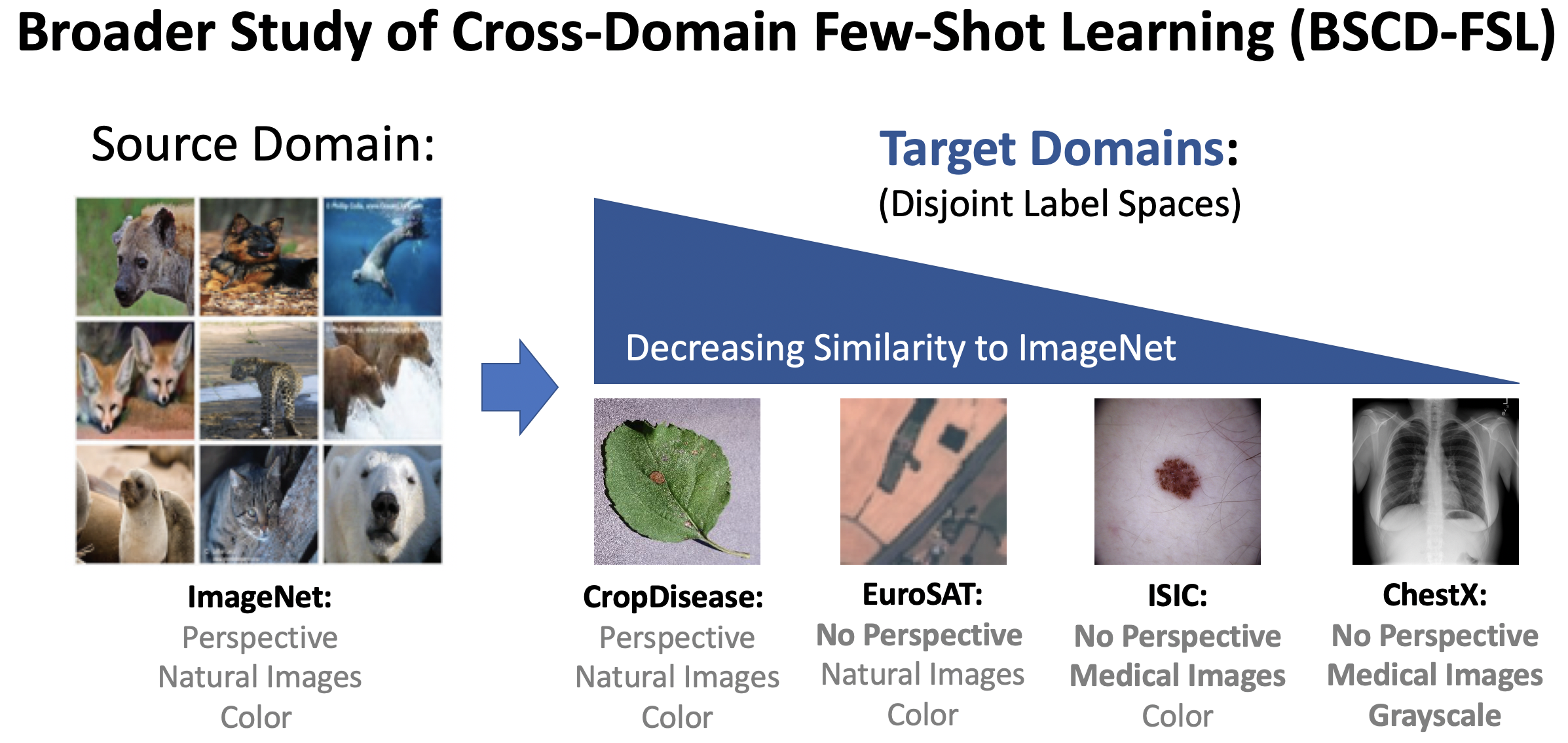
Figure 1: The Broader Study of Cross-Domain Few-Shot Learning (BSCD-FSL) benchmark. ImageNet is used for source training, and domains of varying dissimilarity from natural images are used for target evaluation. Similarity is measured by 3 orthogonal criteria: 1) existence of perspective distortion, 2) the semantic content, and 3) color depth. No data is provided for meta-learning, and target classes are disjoint from the source classes.

Training deep neural networks for visual recognition typically requires a large amount of labelled examples [28]. The generalization ability of deep neural networks relies heavily on the size and variations of the dataset used for training. However, collecting sufficient amounts of data for certain classes may be impossible in practice: for example, in dermatology, there are a multitude of instances of rare diseases, or diseases that become rare for particular types of skin [48, 1, 25]. Or in other domains such as satellite imagery, there are instances of rare categories such as airplane wreckage. Although individually each situation may not carry heavy cost, as a group across many such conditions and modalities, correct identification is critically important, and remains a significant challenge where access to expertise may be impeded.

Although humans generalize to recognize new categories from few examples in certain circumstances, such as when categories exhibit predictable variations across examples and have reasonable contrast from background [32, 31], even humans have trouble recognizing new categories that vary too greatly between examples or differ from prior experience, such as for diagnosis in dermatology, radiology, or other fields [48]. Because there are many applications where learning must work from few examples, and both machines and humans have difficulty learning in these circumstances, finding new methods to tackle the problem remains a challenging but desirable goal.

The problem of learning how to categorize classes with very few training examples has been the topic of the “few-shot learning” field, and has been the subject of a large body of recent work [34, 43, 60, 13, 53, 5, 55]. Few-shot learning is typically composed of the following two stages: meta-learning and meta-testing. In the meta-learning stage, there exists an abundance of base category classes on which a system can be trained to learn well under conditions of few-examples within that particular domain. In the meta-testing stage, a set of novel classes consisting of very few examples per class is used to adapt and evaluate the trained model. However, recent work [5] points out that meta-learning based few-shot learning algorithms underperform compared to traditional pre-training and fine-tuning when there exists a large shift between base and novel class domains. This is a major issue that occurs commonly in practice: by the nature of the problem, collecting data from the same domain for many few-shot classification tasks is difficult. This scenario is referred to as cross-domain few-shot learning, to distinguish it from the conventional few-shot learning setting. Although benchmarks for conventional few-shot learning are well established, the cross-domain few-shot learning evaluation benchmarks are still in early stages. All established works in this space have built cross-domain evaluation benchmarks that are limited to natural images [58, 5, 56]. Under these circumstances, useful knowledge may still be effectively transferring across different domains of natural images, implying that methods designed in this setting may not continue to perform well when applied to domains of other types of images, such as industrial natural images, satellite images, or medical images. Currently, no works study this scenario.

To fill this gap, we propose the Broader Study of Cross-Domain Few-Shot Learning (BSCD-FSL) benchmark (Fig. 1), which covers a spectrum of image types with varying levels of similarity to natural images. Similarity is defined by 3 orthogonal criteria: 1) whether images contain perspective distortion, 2) the semantic content of images, and 3) color depth. The datasets include agriculture images (natural images, but specific to agriculture industry), satellite (loses perspective distortion), dermatology (loses perspective distortion, and contains different semantic content), and radiological images (different according to all 3 criteria). The performance of existing state-of-art meta-learning methods, transfer learning methods, and methods tailored for cross-domain few-shot learning is then rigorously tested on the proposed benchmark.

In summary, the contributions of this paper are itemized as follows:

• We establish a new Broader Study of Cross-Domain Few-Shot Learning (BSCD-FSL) benchmark, consisting of images from a diversity of image types with varying dissimilarity to natural images, according to 1) perspective distortion, 2) the semantic content, and 3) color depth.

• Under these conditions, we extensively evaluate the performance of current meta-learning methods, including methods specifically tailored for cross-domain few-shot learning, as well as variants of fine-tuning.

• The results demonstrate that state-of-art meta-learning methods are outperformed by older meta-learning approaches, and all meta-learning methods underperform in relation to simple fine-tuning by 12.8% average accuracy. In some cases, meta-learning underperforms even networks with random weights.

• Results also show that accuracy gains for cross-domain few-shot learning methods are lost in this new challenging benchmark.

• Finally, we find that accuracy of all methods correlate with the proposed measure of data similarity to natural images, verifying the diversity of the problem representation, and the value of the benchmark towards future research.

We believe this work will help the community understand what methods are most effective in practice, and help drive further advances that can more quickly yield benefit for real-world applications.

2 Related Work

2.0.1 Few-shot learning

Few-shot learning [32, 60, 31] is an increasingly important topic in machine learning. Many few-shot methods have been proposed, including meta-learning, generative and augmentation approaches, semi-supervised methods, and transfer learning.

Meta-learning methods aim to learn models that can be quickly adapted using a few examples [60, 13, 53, 55, 33]. MatchingNet [60] learns an embedding that can map an unlabelled example to its label using a small number of labelled examples, while MAML [13] aims at learning good initialization parameters that can be quickly adapted to a new task. In ProtoNet [53], the goal is to learn a metric space in which classification can be conducted by calculating distances to prototype representations of each class. RelationNet [55] targets learning a deep distance metric to compare a small number of images. More recently, MetaOpt [33] learns feature embeddings that can generalize well under a linear classification rule for novel categories.

The generative and augmentation based family of approaches learn to generate more samples from few examples available for training in a given few-shot learning task. These methods include applying augmentation strategies learned from data [36], synthesizing new data from few examples using a generative model, or using external data for obtaining additional examples that facilitate learning on a given few shot task. In [19, 52] the intra-class relations between pairs of instances of reference categories are modeled in feature space, and then this information is transferred to the novel category instances to generate additional examples in that same feature space. In [63], a generator sub-net is added to a classifier network and is trained to synthesize new examples on the fly in order to improve the classifier performance when being fine-tuned on a novel (few-shot) task. In [44], a few-shot class density estimation is performed with an auto-regressive model, combined with an attention mechanism, where examples are synthesized by a sequential process. In [6, 51, 67] label and attribute semantics are used as additional information for training an example synthesis network.

In some situations there exists additional unlabeled data accompanying the few-shot task. In the semi-supervised few-shot learning [35, 45, 2, 37, 49] the unlabeled data comes in addition to the support set and is assumed to have a similar distribution to the target classes (although some unrelated samples noise is also allowed). In LST [35], self-labeling and soft attention are used on the unlabeled samples intermittently with fine-tuning on the labeled and self-labeled data. Similarly to LST, [45] updates the class prototypes using k-means like iterations initialized from the PN prototypes. In [2], unlabeled examples are used through soft-label propagation. In [15, 37, 24], graph neural networks are used for sharing information between labeled and unlabeled examples in semi-supervised [15, 37] and transductive [24] FSL setting. Notably, in [37] a Graph Construction network is used to predict the task specific graph for propagating labels between samples of semi-supervised FSL task.

Transfer learning [42] is based on the idea of reusing features learned from the base classes for the novel classes, and is conducted mainly by fine-tuning, which adjusts a pre-trained model from a source task to a target task. Yosinski et al. [66] conducted extensive experiments to investigate the transfer utility of pre-trained deep neural networks. In [27], the authors investigated whether higher performing ImageNet models transfer better to new tasks. Ge et al. [16] proposed a selective joint fine-tuning method for improving the performance of models with a limited amount training data. In [18], the authors proposed an adaptive fine-tuning scheme to decide which layers of the pre-trained network should be fine-tuned. Finally, in [10], the authors found that simple transductive fine-tuning beats all prior state-of-art meta-learning approaches.

Common to all few-shot learning methods is the assumption that base classes and novel classes are from the same domain. The current benchmarks for evaluation are miniImageNet [60], CUB [61], Omniglot [31], CIFAR-FS [3] and tieredImageNet [46]. In [56], the authors proposed Meta-Dataset, which is a newer benchmark for training and evaluating few-shot learning algorithms that includes a greater diversity of image content. Although this benchmark is more broad than prior works, the included datasets are still limited to natural images, and both the base classes and novel classes are from the same domain. Recently, [47] proposes a successful meta-learning approach based on conditional neural process on the MetaDataset benchmark.

2.0.2 Domain Adaptation

There is a long history of research in domain adaptation techniques, which aim at transferring knowledge from one or multiple source domains to a target domain with a different data distribution. Early methods have generally relied on the adaptation of shallow classification models, using techniques such as instance re-weighting [12] and model parameter adaptation [65]. More recently, many methods have been proposed to address the problem of domain adaptation using deep neural networks, including discrepancy-based methods, designed to align marginal distributions between the domains [38, 54, 23, 30], adversarial-based approaches, which rely on a domain discriminator to encourage domain-independent feature learning [59, 14], and reconstruction-based techniques, which generally use encoder-decoder models or GANs to reconstruct data in the new domain [4, 69, 22]. All these approaches, however, consider the case that the training and test sets have the same classes. One work considers the scenario where some classes may be disjoint, but still requires class overlap for successful alignment [50]. In contrast, we study the problem of cross-domain few-shot learning, where the source and target domains have completely disjoint label sets.

2.0.3 Cross-domain Few-shot Learning

In cross-domain few-shot learning, base and novel classes are both drawn from different domains, and the class label sets are disjoint. Recent works on cross-domain few-shot learning include analysis of existing meta-learning approaches in the cross-domain setting [5], specialized methods using feature-wise transform to encourage learning representations with improved ability to generalize [58], and works studying cross-domain few-shot learning constrained to the setting of images of items in museum galleries [26]. Common to all these prior works is that they limit the cross-domain setting to the realm of natural images, which still retain a high degree of visual similarity, and do not capture the broader spectrum of image types encountered in practice, such as industrial, aerial, and medical images, where cross-domain few-shot learning techniques are in high demand.

3 Proposed Benchmark

In this section, we introduce the Broader Study of Cross-Domain Few-Shot Learning (BSCD-FSL) benchmark, which includes data from CropDiseases [40], EuroSAT [21], ISIC2018 [57, 8], and ChestX [62] datasets. These datasets cover plant disease images, satellite images, dermoscopic images of skin lesions, and X-ray images, respectively. The selected datasets reflect well-curated real-world use cases for few-shot learning. In addition, collecting enough examples from above domains is often difficult, expensive, or in some cases not possible. Image similarity to natural images is measured by 3 orthogonal criteria: 1) existeence of perspective distortion, 2) the semantic data content, and 3) color depth. According to this criteria, the datasets demonstrate the following spectrum of image types: 1) CropDiseases images are natural images, but are very specialized (similar to existing cross-domain few-shot setting, but specific to agriculture industry), 2) EuroSAT images are less similar as they have lost perspective distortion, but are still color images of natural scenes, 3) ISIC2018 images are even less similar as they have lost perspective distortion and no longer represent natural scenes, and 4) ChestX images are the most dissimilar as they have lost perspective distortion, do not represent natural scenes, and have lost 2 color channels. Example images from ImageNet and the proposed benchmark datasets are shown in Figure 1.

Having a few-shot learning model trained on a source domain such as ImageNet [9] that can generalize to domains such as these, is highly desirable, as it enables effective learning for rare categories in new types of images, which has previously not been studied in detail.

4 Cross-Domain Few-Shot Learning Formulation

The cross domain few-shot learning problem can be formalized as follows. We define a domain as a joint distribution $P$ over input space $\mathcal{X}$ and label space $\mathcal{Y}$. The marginal distribution of $\mathcal{X}$ is denoted as $P_{\mathcal{X}}$. We use the pair $(x,y)$ to denote a sample $x$ and the corresponding label $y$ from the joint distribution $P$. For a model $f_{\theta}$ : $\mathcal{X}$ $\rightarrow$ $\mathcal{Y}$ with parameter $\theta$ and a loss function $\ell$, the expected error is defined as,

$$\epsilon(f_{\theta})=E_{(x,y)\sim P}[\ell(f_{\theta}(x),y)]$$ (1)

In cross-domain few-shot learning, we have a source domain $(\mathcal{X}_{s},\mathcal{Y}_{s})$ and a target domain $(\mathcal{X}_{t},\mathcal{Y}_{t})$ with joint distribution $P_{s}$ and $P_{t}$ respectively, $P_{\mathcal{X}_{s}}\neq P_{\mathcal{X}_{t}}$, and $\mathcal{Y}_{s}$ is disjoint from $\mathcal{Y}_{t}$. The base classes data are sampled from the source domain and the novel classes data are sampled from the target domain. During the training or meta-training stage, the model $f_{\theta}$ is trained (or meta-trained) on the base classes data. During testing (or meta-testing) stage, the model is presented with a support set $S=\{x_{i},y_{i}\}_{i=1}^{K\times N}$ consisting of $N$ examples from $K$ novel classes. This configuration is referred to as “$K$-way $N$-shot” few-shot learning, as the support set has $K$ novel classes and each novel class has $N$ training examples. After the model is adapted to the support set, a query set from novel classes is used to evaluate the model performance.

5 Evaluated Methods for Cross-Domain Few-Shot Learning

In this section, we describe the few-shot learning algorithms that will be evaluated on our proposed benchmark.

5.1 Meta-learning based methods

5.1.1 Single Domain Methods

Meta-learning [13, 43], or learning to learn, aims at learning task-agnostic knowledge in order to efficiently learn on new tasks. Each task $\mathcal{T}_{i}$ is assumed to be drawn from a fixed distribution, $\mathcal{T}_{i}\sim P(\mathcal{T})$. Specially, in few-shot learning, each task $\mathcal{T}_{i}$ is a small dataset $D_{i}\coloneqq\{x_{j},y_{j}\}_{j=1}^{K\times N}$. $P_{s}(\mathcal{T})$ and $P_{t}(\mathcal{T})$ are used to denote the task distribution of the source (base) classes data and target (novel) classes data respectively. During the meta-training stage, the model is trained on $T$ tasks $\{\mathcal{T}_{i}\}_{i=1}^{T}$ which are sampled independently from $P_{s}(\mathcal{T})$. During the meta-testing stage, the model is expected to be quickly adapted to a new task ${T}_{j}\sim P_{t}(\mathcal{T})$.

Meta-learning methods differ in their way of learning the parameter of the initial model $f_{\theta}$ on the base classes data. In MatchingNet [60], the goal is to learn a model $f_{\theta}$ that can map an unlabelled example $\hat{x}$ to its label $\hat{y}$ using a small labelled set $D_{i}\coloneqq\{x_{j},y_{j}\}_{j=1}^{K\times N}$ as $\hat{y}=\sum_{j=1}^{K\times N}a_{\theta}(\hat{x},x_{j})y_{j}$, where $a_{\theta}$ is an attention kernel which leverages $f_{\theta}$ to compute the distance between the unlabelled example $\hat{x}$ and the labelled example $x_{j}$, and $y_{j}$ is the one-hot representation of the label. In contrast, MAML [13] aims at learning an initial parameter $\theta$ that can be quickly adapted to a new task. This is achieved by updating the model parameter via a two-stage optimization process. ProtoNet [53] represents each class $k$ with the mean vector of embedded support examples as $c_{k}=\frac{1}{N}\sum_{j=1}^{N}f_{\theta}(x_{j})$. Classification is then conducted by calculating distance of the example to the prototype representations of each class. In RelationNet [55] the metric of the nearest neighbor classifier is meta-learned using a Siamese Networks trained for optimal comparison between query and support samples. More recently, MetaOpt [33] employs convex base learners and aims at learning feature embeddings that generalize well under a linear classification rule for novel categories. All the existing meta-learning methods implicitly assume that $P_{s}(\mathcal{T})$ = $P_{t}(\mathcal{T})$ so the task-agnostic knowledge learned in the meta-training stage can be leveraged for fast learning on novel classes. However, in cross-domain few-shot learning $P_{s}(\mathcal{T})$ $\neq$ $P_{t}(\mathcal{T})$ which poses severe challenges for current meta-learning methods.

5.1.2 Cross-Domain Methods

Only few methods specifically tailored to learning in the condition of cross-domain few-shot learning have been previously explored, including feaure-wise transform (FWT) [58], and Adversarial Domain Adaptation with Reinforced Sample (ADA-RSS) Selection [11]. Since the problem setting of ADA-RSS requires the existence of unlabelled data in the target domain, we study FWT alone.

FWT is a model agnostic approach that adds a feature-wise transform layer to pre-trained models to learn scale and shift parameters from a collection of several dataset domains, or use parameters empirically determined from a single dataset domain. Both approaches have been previously found to improve performance. Since our benchmark is focused on ImageNet as the single source domain, we focus on the single data domain approach. The method is studied in combination with all meta-learning algorithms described in the prior section.

5.2 Transfer learning based methods

An alternative way to tackle the problem of few-shot learning is based on transfer learning, where an initial model $f_{\theta}$ is trained on the base classes data in a standard supervised learning way and reused on the novel classes. There are several options to realize the idea of transfer learning for few-shot learning:

5.2.1 Single Model Methods

In this paper, we extensively evaluate the following commonly variants of single model fine-tuning:

• Fixed feature extractor (Fixed): simply leverage the pre-trained model as a fixed feature extractor.

• Fine-tuning all layers (Ft All): adjusts all the pre-trained parameters on the new task with standard supervised learning.

• Fine-tuning last-k (Ft Last-k): only the last $k$ layers of the pre-trained model are optimized for the new task. In the paper, we consider Fine-tuning last-1, Fine-tuning last-2, Fine-tuning last-3.

• Transductive fine-tuning (Transductive Ft): in transductive fine-tuning, the statistics of the query images are used via batch normalization [10]. [41].

In addition, we compare these single model transfer learning techniques against a baseline of an embedding formed by a randomly initialized network (termed Random) to contrast against a fixed feature vector that has no pre-training. All the variants of single model fine-tuning are based on linear classifier but differ in their approach to fine-tune the single model feature extractor.

Another line of work for few-shot learning uses a broader variety of classifiers for transfer learning. For example, recent works show that mean-centroid classifier and cosine-similarity based classifier are more effective than linear classifier for few-shot learning [39, 5]. Therefore we study these two variations as well.

Mean-centroid classifier.

The mean-centroid classifier is inspired from ProtoNet [53]. Given the pre-trained model $f_{\theta}$ and a support set $S=\{x_{i},y_{i}\}_{i=1}^{K\times N}$, where $K$ is the number of novel classes and $N$ is the number of images per class. The class prototypes are computed in the same way as in ProtoNet. Then the likelihood of an unlabelled example $\hat{x}$ belongs to class $k$ is computed as,

$$p(y=k|\hat{x})=\frac{\textnormal{exp}(-d(f_{\theta},c_{k}))}{\sum_{l=1}^{K}\textnormal{exp}(-d(f_{\theta},c_{l}))}$$ (2)

where $d()$ is a distance function. In the experiments, we use negative cosine similarity. Different from ProtoNet, $f_{\theta}$ is pretrained on the base classes data in a standard supervised learning way.

Cosine-similarity based classifier.

In cosine-similarity based classifier, instead of directly computing the class prototypes using the pre-trained model, each class $k$ is represented as a $d$-dimension weight vector $\mathbf{w}_{k}$ which is initialized randomly. For each unlabeled example $\hat{x}_{i}$, the cosine similarity to each weight vector is computed as $c_{i,k}=\frac{f_{\theta}(\hat{x}_{i})^{T}\mathbf{w}_{k}}{\lVert f_{\theta}(\hat{x}_{i})\rVert\lVert\mathbf{w}_{k}\rVert}$. The predictive probability of the example $\hat{x}_{i}$ belongs to class $k$ is computed by normalizing the cosine similarity with a softmax function. Intuitively, the weight vector $\mathbf{w}_{k}$ can be thought as the prototype of class $k$.

5.2.2 Transfer from Multiple Pre-trained Models

In this section, we describe a straightforward method that utilizes multiple models pre-trained on source domains of natural images similar to ImageNet. Note that all domains are still disjoint from the target datasets for the cross-domain few-shot learning setting. The purpose is to measure how much performance may improve by utilizing an ensemble of models trained from data that is different from the target domain. The described method requires no change to how models are trained and is an off-the-shelf solution to leverage existing pre-trained models for cross-domain few-shot learning, without requiring access to the source datasets.

Assume we have a library of $C$ pre-trained models $\{M_{c}\}_{c=1}^{C}$ which are trained on various datasets in a standard way. We denote the layers of all pre-trained models as a set $F$. Given a support set $S=\{x_{i},y_{i}\}_{i=1}^{K\times N}$ where $(x_{i},y_{i})\sim P_{t}$, our goal is to find a subset $I$ of the layers to generate a feature vector for each example in order to achieve the lowest test error. Mathematically,

$$\operatorname*{arg\,min}_{I\subseteq F}\,{}_{(x,y)\sim\ P_{t}}\ell(f_{s}(T(\{l(x):l\in I\}),y)$$ (3)

where $\ell$ is a loss function, $T()$ is a function which concatenates a set of feature vectors, $l$ is one particular layer in the set $I$, and $f_{s}$ is a linear classifier. Practically, for feature vectors $l$ coming from inner layers which are three-dimensional, we convert them to one-dimensional vectors by using Global Average Pooling. Since Eq. 3 is intractable generally, we instead adopt a two-stage greedy selection method, called Incremental Multi-model Selection, to iteratively find the best subset of layers for a given support $S$.

In the first stage, for each pre-trained model, we a train linear classifier on the feature vector generated by each layer individually and select the corresponding layer which achieves the lowest average error using five-fold cross-validation on the support set $S$. Essentially, the goal of the first stage is to find the most effective layer of each pre-trained model given the task in order to reduce the search space and mitigate risk of overfitting. For convenience, we denote the layers selected in the first selection stage as set $I_{1}$. In the second stage, we greedily add the layers in $I_{1}$ into the set $I$ following a similar cross-validation procedure. First, we add the layer in $I_{1}$ into $I$ which achieves the lowest cross-validation error. Then we iterate over $I_{1}$, and add each remaining layer into $I$ if the cross-validation error is reduced when the new layer is added. Finally, we concatenate the feature vector generated by each layer in set $I$ and train the final linear classifier. Please see Algorithm 1 in Appendix for further details.

Methods	ChestX			ISIC
	5-way 5-shot	5-way 20-shot	5-way 50-shot	5-way 5-shot	5-way 20-shot	5-way 50-shot
MatchingNet	22.40% $\pm$ 0.7%	23.61% $\pm$ 0.86%	22.12% $\pm$ 0.88%	36.74% $\pm$ 0.53%	45.72% $\pm$ 0.53%	54.58% $\pm$ 0.65%
MatchingNet+FWT	21.26% $\pm$ 0.31%	23.23% $\pm$ 0.37%	23.01% $\pm$ 0.34%	30.40% $\pm$ 0.48%	32.01% $\pm$ 0.48%	33.17% $\pm$ 0.43%
MAML	23.48% $\pm$ 0.96%	27.53% $\pm$ 0.43%	-	40.13% $\pm$ 0.58%	52.36% $\pm$ 0.57%	-
ProtoNet	24.05% $\pm$ 1.01%	28.21% $\pm$ 1.15%	29.32% $\pm$ 1.12%	39.57% $\pm$ 0.57%	49.50% $\pm$ 0.55%	51.99% $\pm$ 0.52%
ProtoNet+FWT	23.77% $\pm$ 0.42%	26.87% $\pm$ 0.43%	30.12% $\pm$ 0.46%	38.87% $\pm$ 0.52%	43.78% $\pm$ 0.47%	49.84% $\pm$ 0.51%
RelationNet	22.96% $\pm$ 0.88%	26.63% $\pm$ 0.92%	28.45% $\pm$ 1.20%	39.41% $\pm$ 0.58%	41.77% $\pm$ 0.49%	49.32% $\pm$ 0.51%
RelationNet+FWT	22.74% $\pm$ 0.40%	26.75% $\pm$ 0.41%	27.56% $\pm$ 0.40%	35.54% $\pm$ 0.55%	43.31% $\pm$ 0.51%	46.38% $\pm$ 0.53%
MetaOpt	22.53% $\pm$ 0.91%	25.53% $\pm$ 1.02%	29.35% $\pm$ 0.99%	36.28% $\pm$ 0.50%	49.42% $\pm$ 0.60%	54.80% $\pm$ 0.54%

Methods	EuroSAT			CropDiseases
	5-way 5-shot	5-way 20-shot	5-way 50-shot	5-way 5-shot	5-way 20-shot	5-way 50-shot
MatchingNet	64.45% $\pm$ 0.63%	77.10% $\pm$ 0.57%	54.44% $\pm$ 0.67%	66.39% $\pm$ 0.78%	76.38% $\pm$ 0.67%	58.53% $\pm$ 0.73%
MatchingNet+FWT	56.04% $\pm$ 0.65%	63.38% $\pm$ 0.69%	62.75% $\pm$ 0.76%	62.74% $\pm$ 0.90%	74.90% $\pm$ 0.71%	75.68% $\pm$ 0.78%
MAML	71.70% $\pm$ 0.72%	81.95% $\pm$ 0.55%	-	78.05% $\pm$ 0.68%	89.75% $\pm$ 0.42%	-
ProtoNet	73.29% $\pm$ 0.71%	82.27% $\pm$ 0.57%	80.48% $\pm$ 0.57%	79.72% $\pm$ 0.67%	88.15% $\pm$ 0.51%	90.81% $\pm$ 0.43%
ProtoNet+FWT	67.34% $\pm$ 0.76%	75.74% $\pm$ 0.70%	78.64% $\pm$ 0.57%	72.72% $\pm$ 0.70%	85.82% $\pm$ 0.51%	87.17% $\pm$ 0.50%
RelationNet	61.31% $\pm$ 0.72%	74.43% $\pm$ 0.66%	74.91% $\pm$ 0.58%	68.99% $\pm$ 0.75%	80.45% $\pm$ 0.64%	85.08% $\pm$ 0.53%
RelationNet+FWT	61.16% $\pm$ 0.70%	69.40% $\pm$ 0.64%	73.84% $\pm$ 0.60%	64.91% $\pm$ 0.79%	78.43% $\pm$ 0.59%	81.14% $\pm$ 0.56%
MetaOpt	64.44% $\pm$ 0.73%	79.19% $\pm$ 0.62%	83.62% $\pm$ 0.58%	68.41% $\pm$ 0.73%	82.89% $\pm$ 0.54%	91.76% $\pm$ 0.38%

Table 1: The results of meta-learning methods on the proposed benchmark.

6 Evaluation Setup

For meta-learning methods, we meta-train all meta-learning methods on the base classes of miniImageNet [60] and meta-test the trained models on each dataset of the proposed benchmark. For transfer learning methods, we train the pre-trained model on base classes of miniImageNet. For transferring from multiple pre-trained models, we use a maximum of five pre-trained models, trained on miniImagenet, CIFAR100 [29], DTD [7], CUB [64], Caltech256 [17], respectively. On all experiments we consider 5-way 5-shot, 5-way 20-shot, 5-way 50-shot. For all cases, the test (query) set has 15 images per class. All experiments are performed with ResNet-10 [20] for fair comparison. For each evaluation, we use the same 600 randomly sampled few-shot episodes (for consistency), and report the average accuracy and $95\%$ confidence interval.

During the training (meta-training) stage, models used for transfer learning and meta-learning models are both trained for 400 epochs with Adam optimizer. The learning rate is set to 0.001. During testing (meta-testing), both transfer learning methods and those meta-learning methods that require adaptation on the support set of the test episodes (MAML, RelationNet, etc.) use SGD with momentum. The learning rate is 0.01 and the momentum rate is 0.9. All variants of fine-tuning methods are trained for 100 epochs. For feature-wise transformation [58], we adopt the recommended hyperparameters in the original paper for meta-training from one source domain . In the training or meta-training stage, we apply standard data augmentation including random crop, random flip, and color jitter.

In the cross-domain few-shot learning setting, since the source domain and target domain are drastically different, it may not be appropriate to use the source domain data for hyperparameter tuning or validation. Therefore, we leave the question of how to determine the best hyperparameters in the cross-domain few-shot learning as future work. One simple strategy is to use the test set or validation set of the source domain data for hyperparameter tuning. More sophisticated methods may use datasets that are similar to the target domain data.

7 Experimental Results

7.1 Meta-learning based results

Table 1 show the results on the proposed benchmark of meta-learning, for each dataset, method, and shot level in the benchmark. Across all datasets and shot levels, the average accuracies (and 95% confidence internals) are 50.21% (0.70) for MatchingNet, 46.55% (0.58) for MatchingNet+FWT, 38.75% (0.41) for MAML, 59.78% (0.70) for ProtoNet, 56.72% (0.55) for ProtoNet+FWT, 54.48% (0.71) for RelationNet, 52.6% (0.56) for RelationNet+FWT, and 57.35% (0.68) for MetaOpt. The performance of MAML was impacted by its inability to scale to larger shot levels due to memory overflow. Methods paired with Feature-Wise Transform are marked with “+FWT”.

What is immediately apparent from Table 1, is that the prior state-of-art MetaOptNet is no longer state-of-art, as it is outperformed by ProtoNet. In addition, methods designed specifically for cross-domain few-shot learning lead to consistent performance degradation in this new challenging benchmark. Finally, performance in general strongly positively correlates to the dataset’s similarity to ImageNet, confirming that the benchmark’s intentional design allows us to investigate few-shot learning in a spectrum of cross-domain difficulties.

Methods	ChestX			ISIC
	5-way 5-shot	5-way 20-shot	5-way 50-shot	5-way 5-shot	5-way 20-shot	5-way 50-shot
Random	21.80% $\pm$ 1.03%	25.69% $\pm$ 0.95%	26.19% $\pm$ 0.94%	37.91% $\pm$ 1.39%	47.24% $\pm$ 1.50%	50.85% $\pm$ 1.37%
Fixed	25.35% $\pm$ 0.96%	30.83% $\pm$ 1.05%	36.04% $\pm$ 0.46%	43.56% $\pm$ 0.60%	52.78% $\pm$ 0.58%	57.34% $\pm$ 0.56%
Ft All	25.97% $\pm$ 0.41%	31.32% $\pm$ 0.45%	35.49% $\pm$ 0.45%	48.11% $\pm$ 0.64%	59.31% $\pm$ 0.48%	66.48% $\pm$ 0.56%
Ft Last-1	25.96% $\pm$ 0.46%	31.63% $\pm$ 0.49%	37.03% $\pm$ 0.50%	47.20% $\pm$ 0.45%	59.95% $\pm$ 0.45%	65.04% $\pm$ 0.47%
Ft Last-2	26.79% $\pm$ 0.59%	30.95% $\pm$ 0.61%	36.24% $\pm$ 0.62%	47.64% $\pm$ 0.44%	59.87% $\pm$ 0.35%	66.07% $\pm$ 0.45%
Ft Last-3	25.17% $\pm$ 0.56%	30.92% $\pm$ 0.89%	37.27% $\pm$ 0.64%	48.05% $\pm$ 0.55%	60.20% $\pm$ 0.33%	66.21% $\pm$ 0.52%
Transductive Ft	26.09% $\pm$ 0.96%	31.01% $\pm$ 0.59%	36.79% $\pm$ 0.53%	49.68% $\pm$ 0.36%	61.09% $\pm$ 0.44%	67.20% $\pm$ 0.59%

Methods	EuroSAT			CropDiseases
	5-way 5-shot	5-way 20-shot	5-way 50-shot	5-way 5-shot	5-way 20-shot	5-way 50-shot
Random	58.00% $\pm$ 2.01%	68.93% $\pm$ 1.47%	71.65% $\pm$ 1.47%	69.68% $\pm$ 1.72%	83.41% $\pm$ 1.25%	86.56% $\pm$ 1.42%
Fixed	75.69% $\pm$ 0.66%	84.13% $\pm$ 0.52%	86.62% $\pm$ 0.47%	87.48% $\pm$ 0.58%	94.45% $\pm$ 0.36%	96.62% $\pm$ 0.25%
Ft All	79.08% $\pm$ 0.61%	87.64% $\pm$ 0.47%	90.89% $\pm$ 0.36%	89.25% $\pm$ 0.51%	95.51% $\pm$ 0.31%	97.68% $\pm$ 0.21%
Ft Last-1	80.45% $\pm$ 0.54%	87.92% $\pm$ 0.44%	91.41% $\pm$ 0.46%	88.72% $\pm$ 0.53%	95.76% $\pm$ 0.65%	97.87% $\pm$ 0.48%
Ft Last-2	79.57% $\pm$ 0.51%	87.67% $\pm$ 0.46%	90.93% $\pm$ 0.45%	88.07% $\pm$ 0.56%	95.68% $\pm$ 0.76%	97.64% $\pm$ 0.59%
Ft Last-3	78.04% $\pm$ 0.77%	87.52% $\pm$ 0.53%	90.83% $\pm$ 0.42%	89.11% $\pm$ 0.47%	95.31% $\pm$ 0.7%	97.45% $\pm$ 0.46%
Transductive Ft	81.76% $\pm$ 0.48%	87.97% $\pm$ 0.42%	92.00% $\pm$ 0.56%	90.64% $\pm$ 0.54%	95.91% $\pm$ 0.72%	97.48% $\pm$ 0.56%

Table 2: The results of different variants of single model fine-tuning on the proposed benchmark.

7.2 Transfer learning based results

7.2.1 Single model results

Table 2 show the results on the proposed benchmark of various single model transfer learning methods. Across all datasets and shot levels, the average accuracies (and 95% confidence internals) are 53.99% (1.38) for random embedding, 64.24 (0.59) for fixed feature embedding, 67.23% (0.46) for fine-tuning all layers, 67.41% (0.49) for fine-tuning the last 1 layer, 67.26% (0.53) for fine-tuning the last 2 layers, 67.17% (0.58) for fine-tuning the last 3 layers, and 68.14% (0.56) for transductive fine-tuning. From these results, several observations can be made. The first observation is that, although meta-learning methods have been previously shown to achieve higher performance than transfer learning in the standard few-shot learning setting [60, 5], in the cross-domain few-shot learning setting this situation is reversed: meta-learning methods significantly underperform simple fine-tuning methods. In fact, MatchingNet performs worse than a randomly generated fixed embedding. A possible explanation is that meta-learning methods are fitting the task distribution on the base class data, improving performance in that circumstance, but hindering ability to generalize to another task distribution. The second observation is that, by leveraging the statistics of the test data, transductive fine-tuning continues to achieve higher results than the standard fine-tuning and meta-learning, as previously reported [10]. While transductive fine-tuning, however, assumes that all the queries are available as unlabeled data. The third observation is that the accuracy of most methods on the benchmark continues to be dependent on how similar the dataset is to ImageNet: CropDiseases commands the highest performance on average, while EuroSAT follows in 2^nd place, ISIC in 3^rd, and ChestX in 4^th. This further supports the motivation behind benchmark design in targeting applications with increasing visual domain dissimilarity to natural images.

Table 3 shows results from varying the classifier. While mean-centriod classifier and cosine-similarity classifier are shown to be more efficient than simple linear classifier in the conventional few-shot learning setting, our results show that mean-centroid and cosine-similarity classifier only have a marginal advantage on ChestX and EuroSAT over linear classifier in the 5-shot case (Table 3). As the shot increases, linear classifier begins to dominate mean-centroid and cosine-similarity classifier. One plausible reason is that since both mean-centroid and cosine-similarity classifier conduct classification based on unimodal class prototypes, when the number of examples increases, unimodal distribution becomes less suitable, and multi-modal distribution is required.

Methods	ChestX			ISIC
	5-way 5-shot	5-way 20-shot	5-way 50-shot	5-way 5-shot	5-way 20-shot	5-way 50-shot
Linear	25.97% $\pm$ 0.41%	31.32% $\pm$ 0.45%	35.49% $\pm$ 0.45%	48.11% $\pm$ 0.64%	59.31% $\pm$ 0.48%	66.48% $\pm$ 0.56%
Mean-centroid	26.31% $\pm$ 0.42%	30.41% $\pm$ 0.46%	34.68% $\pm$ 0.46%	47.16% $\pm$ 0.54%	56.40% $\pm$ 0.53%	61.57% $\pm$ 0.66%
Cosine-similarity	26.95% $\pm$ 0.44%	32.07% $\pm$ 0.55%	34.76% $\pm$ 0.55%	48.01% $\pm$ 0.49%	58.13% $\pm$ 0.48%	62.03% $\pm$ 0.52%

Methods	EuroSAT			CropDiseases
	5-way 5-shot	5-way 20-shot	5-way 50-shot	5-way 5-shot	5-way 20-shot	5-way 50-shot
Linear	79.08% $\pm$ 0.61%	87.64% $\pm$ 0.47%	91.34% $\pm$ 0.37%	89.25% $\pm$ 0.51%	95.51% $\pm$ 0.31%	97.68% $\pm$ 0.21%
Mean-centroid	82.21% $\pm$ 0.49%	87.62% $\pm$ 0.34%	88.24% $\pm$ 0.29%	87.61% $\pm$ 0.47%	93.87% $\pm$ 0.68%	94.77% $\pm$ 0.34%
Cosine-similarity	81.37% $\pm$ 1.54%	86.83% $\pm$ 0.43%	88.83% $\pm$ 0.38%	89.15% $\pm$ 0.51%	93.96% $\pm$ 0.46%	94.27% $\pm$ 0.41%

Table 3: The results of varying the classifier for fine-tuning on the proposed benchmark.

We further analyze how layers are changed during transfer. We use $\theta$ to denote the original pre-trained parameters and $\hat{\theta}$ to denote the parameters after fine-tuning. Figure 2 shows the relative parameter change of the ResNet10 miniImageNet pre-trained model as $\frac{|\theta-\hat{\theta}|}{|\theta|}$, averaged over all parameters per layer, and 100 runs. Several interesting observations can be made from these results. First, across all the datasets and all the shots, the first layer of the pre-trained model changes most. This indicates that if the target domain is different from the source domain, the lower layers of the pre-trained models still need to be adjusted. Second, while the datasets are drastically different, we observe that some layers are consistently more transferable than other layers. One plausible explanation for this phenomenon is the heterogeneous characteristic of layers in overparameterized deep neural networks [68].

Methods	ChestX			ISIC
	5-way 5-shot	5-way 20-shot	5-way 50-shot	5-way 5-shot	5-way 20-shot	5-way 50-shot
All embeddings	26.74% $\pm$ 0.42%	32.77% $\pm$ 0.47%	38.07% $\pm$ 0.50%	46.86% $\pm$ 0.60%	58.57% $\pm$ 0.59%	66.04% $\pm$ 0.56%
IMS-f	25.50% $\pm$ 0.45%	31.49% $\pm$ 0.47%	36.40% $\pm$ 0.50%	45.84% $\pm$ 0.62%	61.50% $\pm$ 0.58%	68.64% $\pm$ 0.53%

Methods	EuroSAT			CropDiseases
	5-way 5-shot	5-way 20-shot	5-way 50-shot	5-way 5-shot	5-way 20-shot	5-way 50-shot
All embeddings	81.29% $\pm$ 0.62%	89.90% $\pm$ 0.41%	92.76% $\pm$ 0.34%	90.82% $\pm$ 0.48%	96.64% $\pm$ 0.25%	98.14% $\pm$ 0.18%
IMS-f	83.56% $\pm$ 0.59%	91.22% $\pm$ 0.38%	93.85% $\pm$ 0.30%	90.66% $\pm$ 0.48%	97.18% $\pm$ 0.24%	98.43% $\pm$ 0.16%

Table 4: The results of using all embeddings, and the Incremental Multi-model Selection (IMS-f) based on fine-tuned pre-trained models on the proposed benchmark.

7.2.2 Transfer from Multiple Pre-trained Models

The results of the described Incremental Muiti-model Selection are shown in Table 4. IMS-f fine-tunes each pre-trained model before applying the model selection. We include a baseline called all embeddings which concatenates the feature vectors generated by all the layers from the fine-tuned models. Across all datasets and shot levels, the average accuracies (and 95% confidence internals) are 68.22% (0.45) for all embeddings, and 68.69% (0.44) for IMS-f. The results show that IMS-f generally improves upon all embeddings which indicates the importance of selecting relevant pre-trained models to the target dataset. Model complexity also tends to decrease by over 20% compared to all embeddings on average. We can also observe that it is beneficial to use multiple pre-trained models than using just one model, even though these models are trained from data in different domains and different image types. Compared with standard finetuning with a linear classifier, the average improvement of IMS-f across all the shots on ChestX is 0.20%, on ISIC is 0.69%, on EuroSAT is 3.52% and on CropDiseases is 1.27%.

In further analysis, we study the effect of the number of pre-trained models for the studied multi-model selection method. We consider libraries consisting of two, three, four, and all five pre-trained models. The pre-trained models are added into the library in the order of ImageNet, CIFAR100, DTD, CUB, Caltech256. For each dataset, the experiment is conducted on 5-way 50-shot with 600 episodes. The results are shown in Table 5. As more pre-trained models are added into the library, we can observe that the test accuracy on ChestX and ISIC gradually improves which can be attributed to the diverse features provided by different pre-trained models. However, on EuroSAT and CropDiseases, only a marginal improvement can be observed. One possible reason is that the features from ImageNet already captures the characteristics of the datasets and more pre-trained models does not provide additional information.

Finally, we visualize for each dataset which pre-trained models are selected in the studied incremental multi-model selection. The experiments are conducted on 5-way 50-shot with all five pre-trained models. For each dataset, we repeat the experiments for 600 episodes and calculate the frequency of each model being selected. The results are shown in Figure 3. We observe the distribution of the frequency differs significantly across datasets, as target datasets can benefit from different pre-trained models.

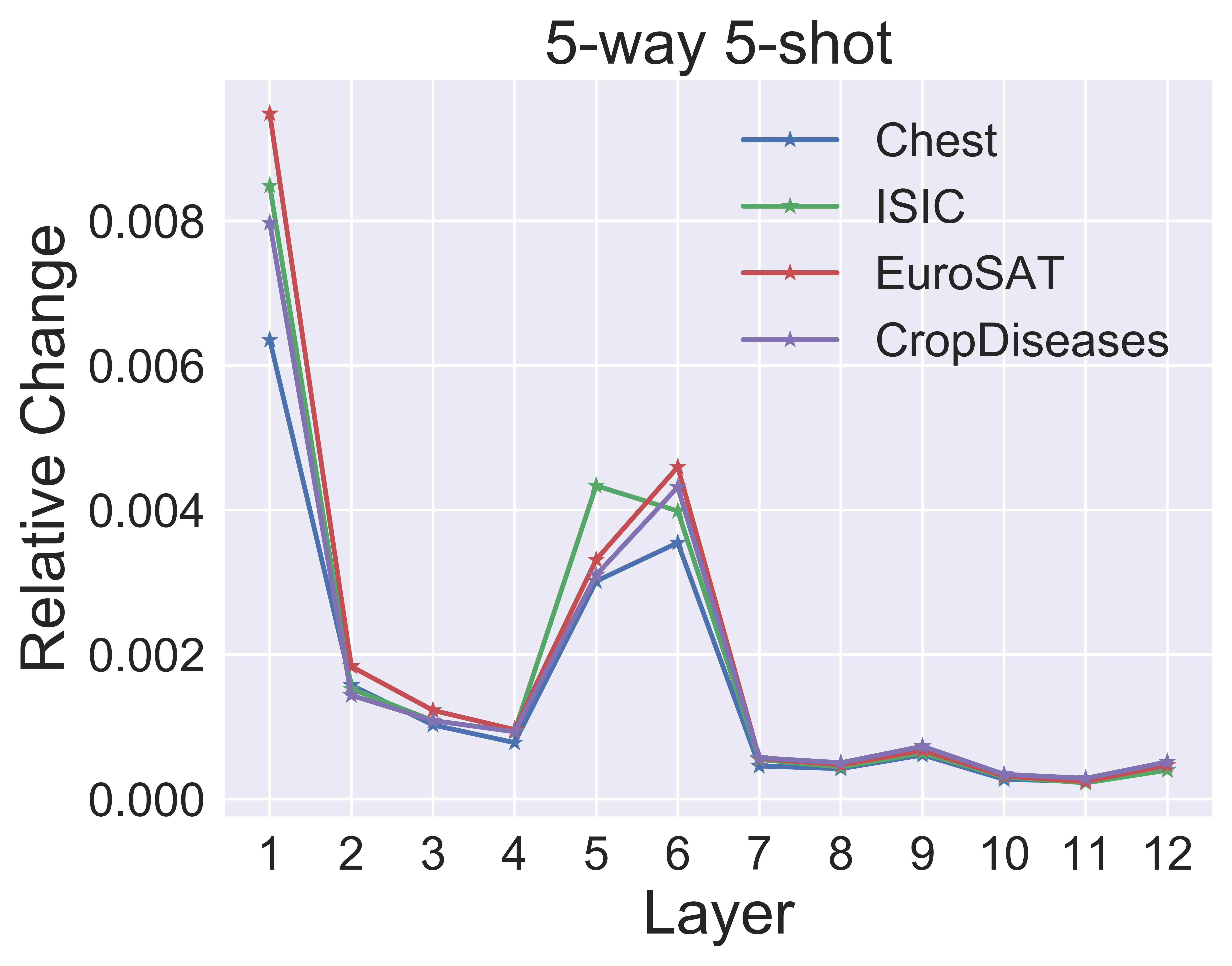
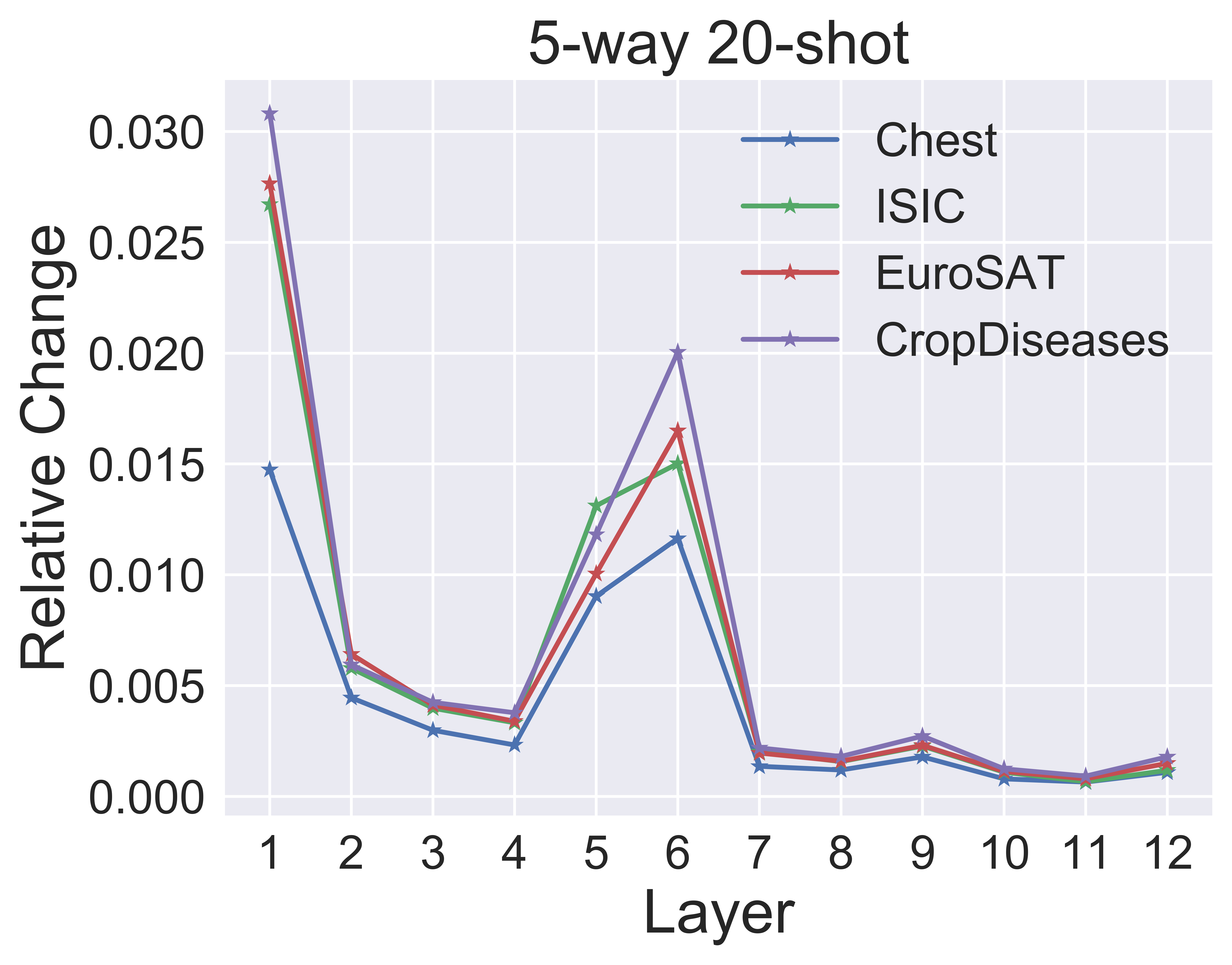
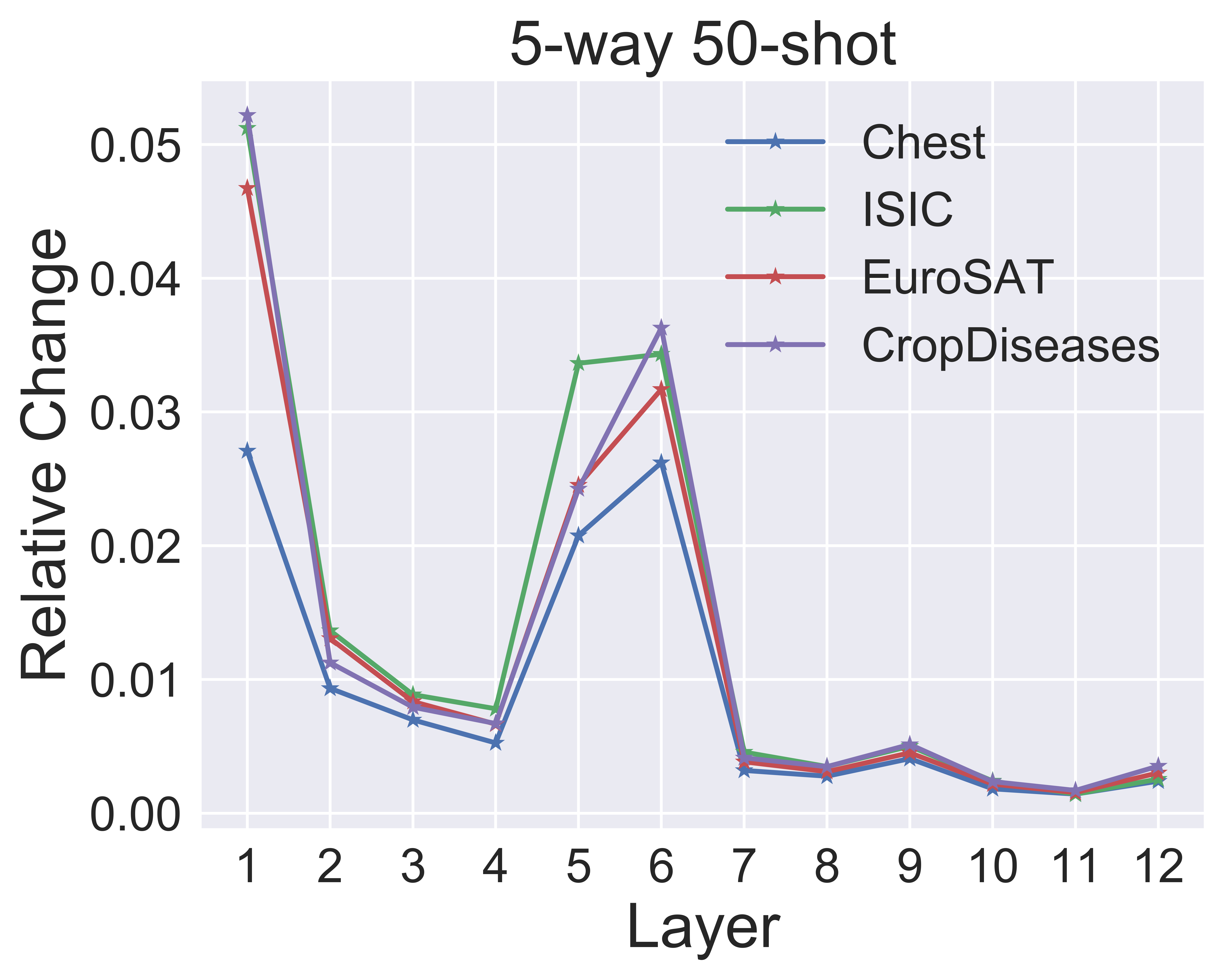
Figure 2: Relative change of pre-trained network layers for single model transfer.

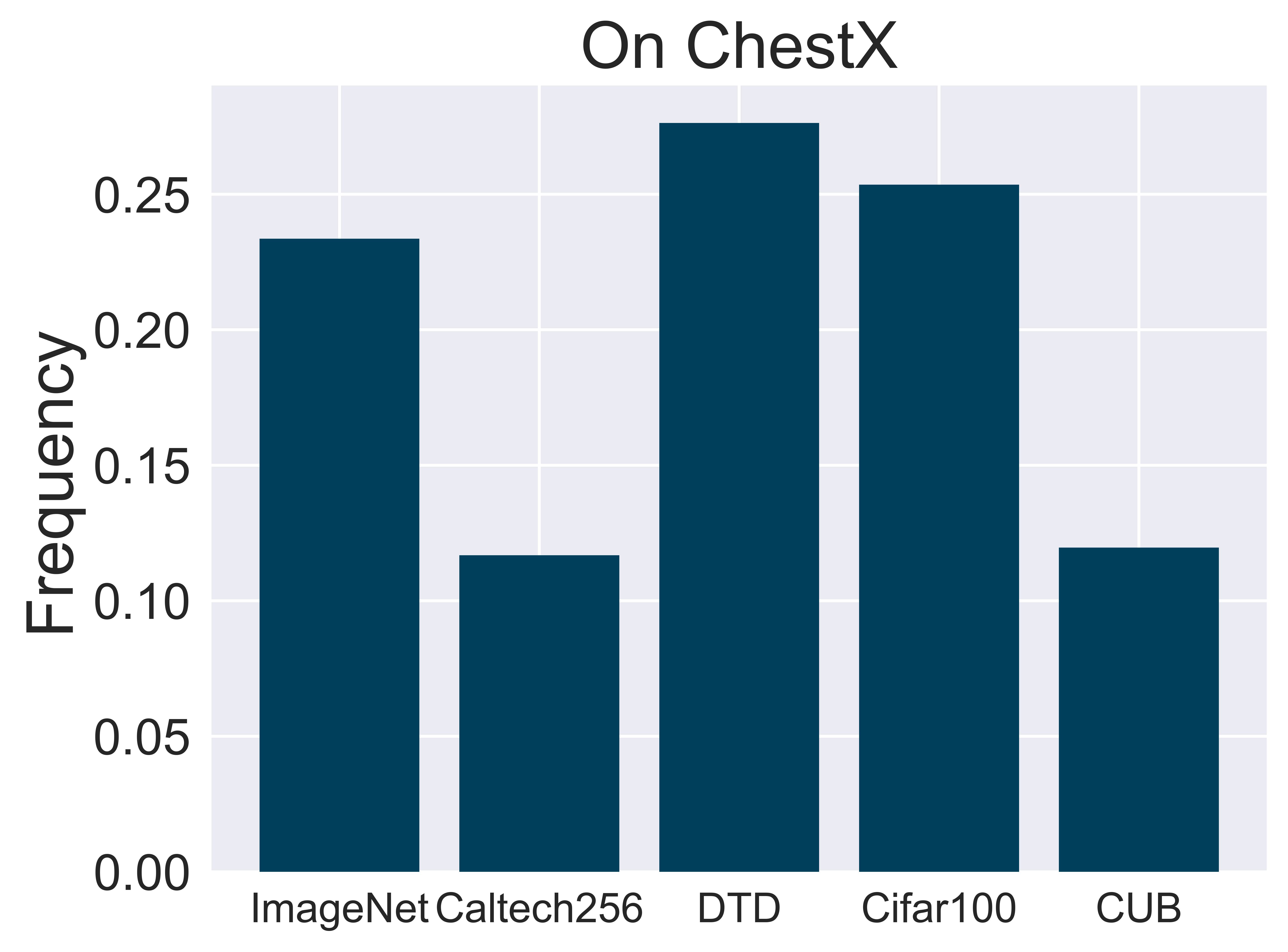
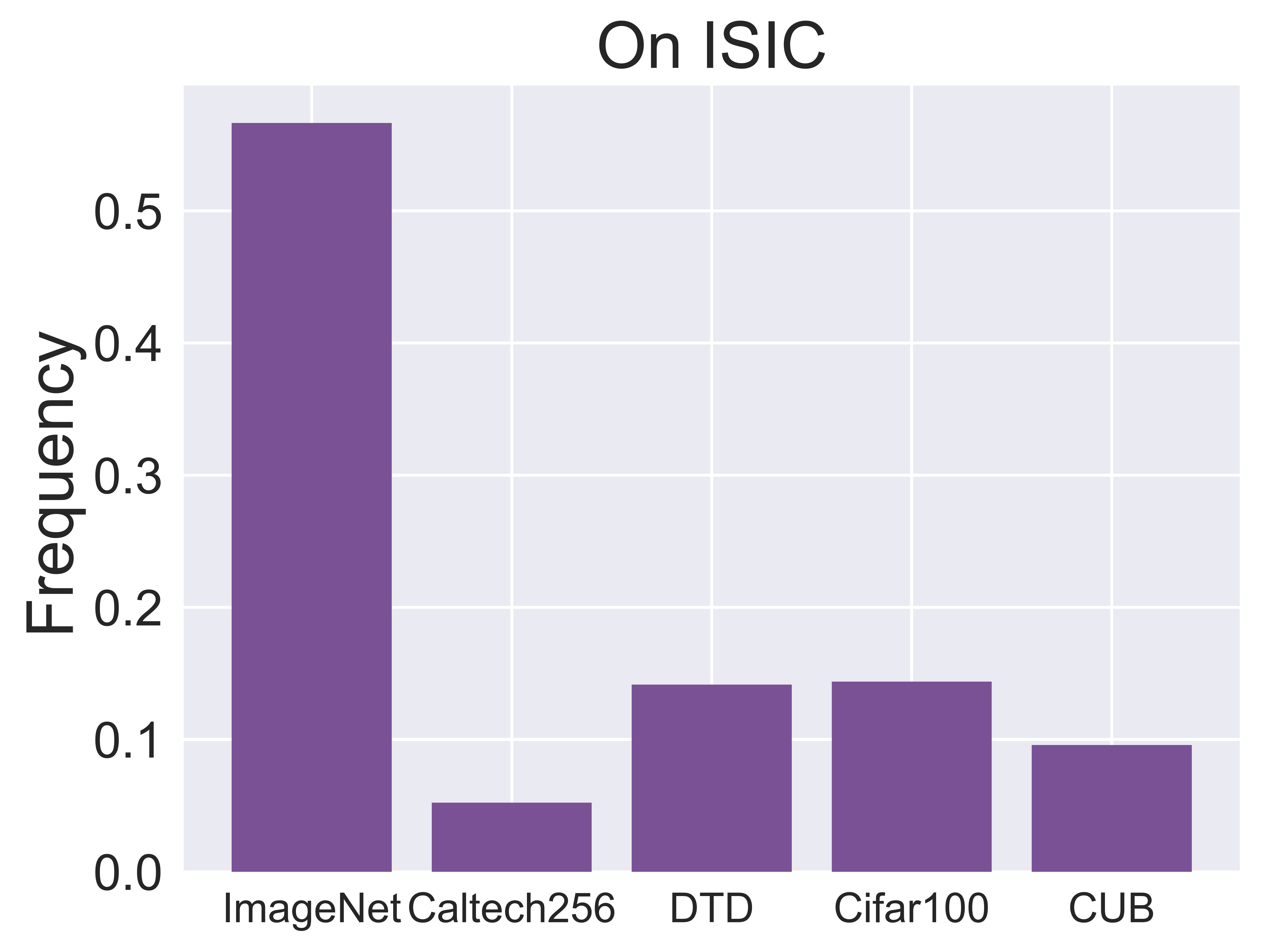
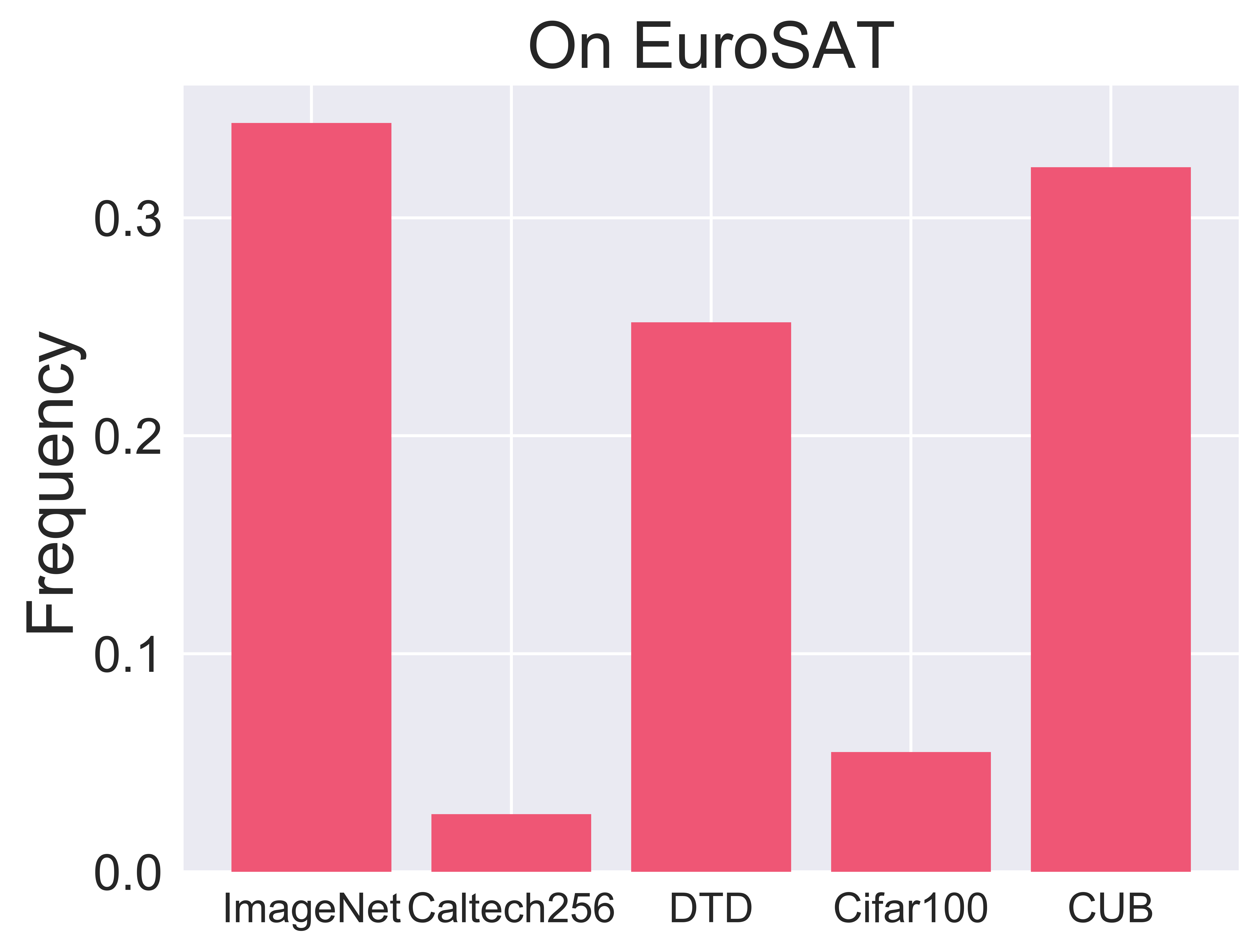
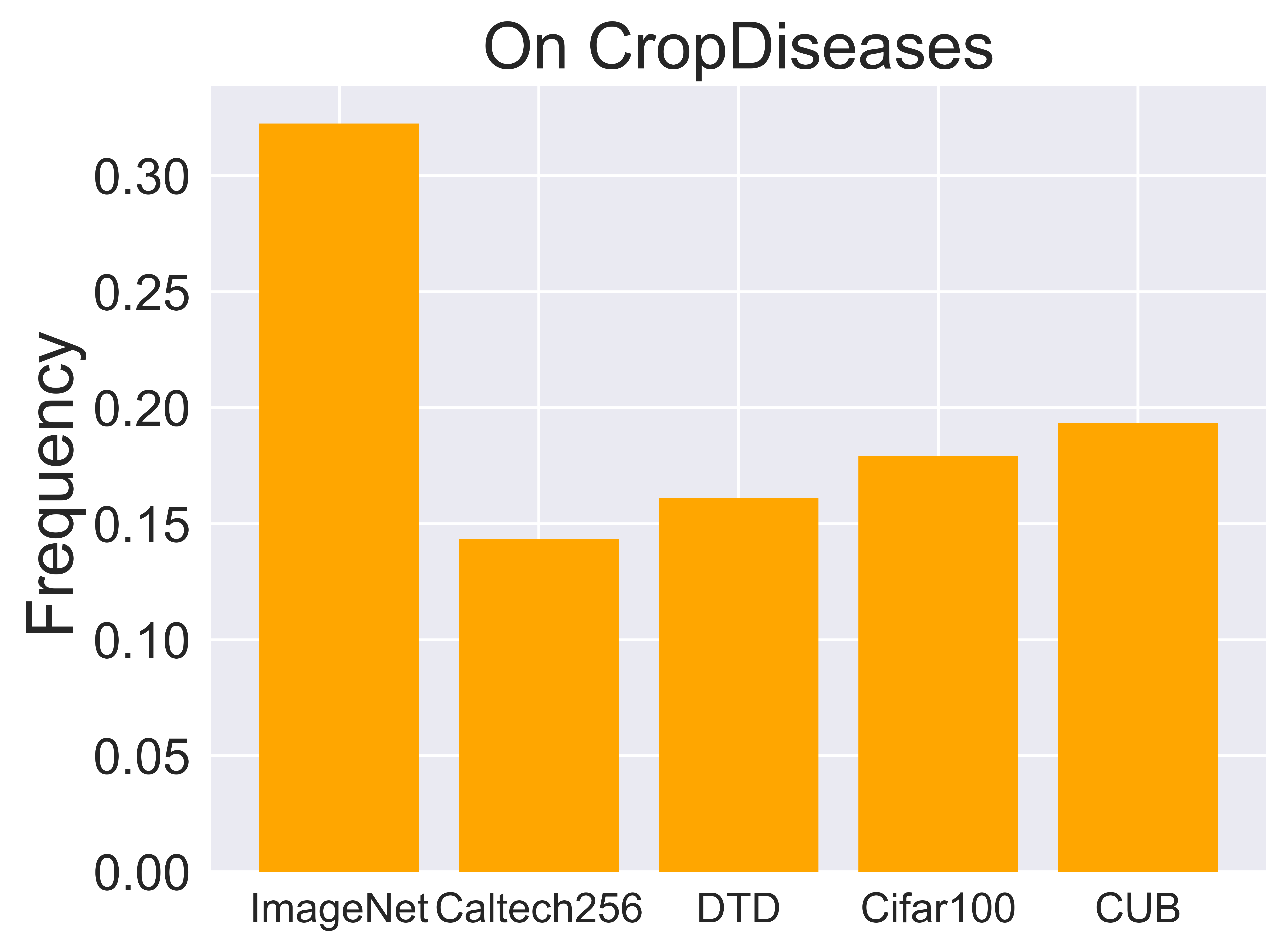
Figure 3: Frequency of source model selection for each dataset in the benchmark.

	2	3	4	5
ChestX	34.35%	36.29%	37.64%	37.89%
ISIC	59.4%	62.49%	65.07%	64.77%
EuroSAT	91.71%	93.49%	92.67%	93.00%
CropDiseases	98.43%	98.09%	98.05%	98.60%

Table 5: Number of models’ effect on test accuracy.

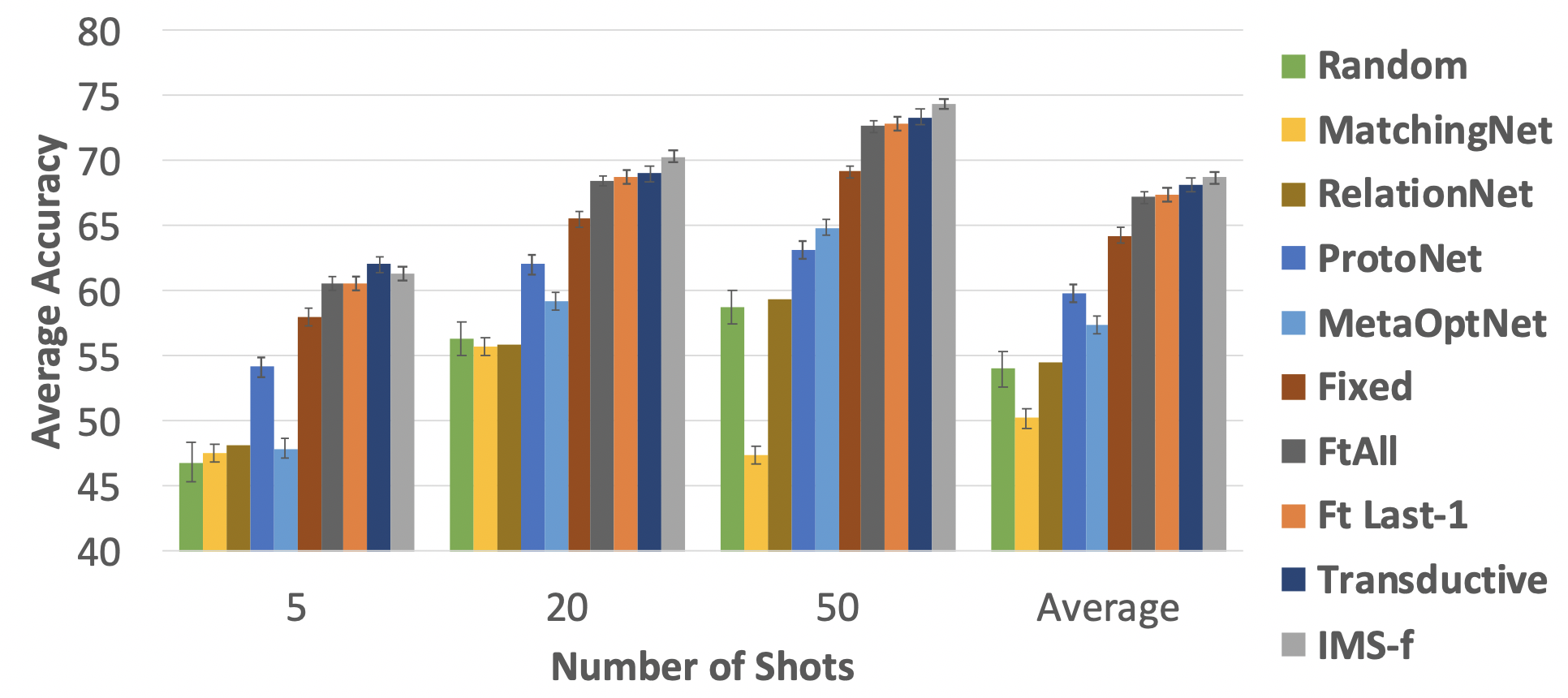
Figure 4: Comparisons of methods across the entire benchmark.

7.3 Benchmark Summary

Figure 4 summarizes the comparison across algorithms, according to the average accuracy across all datasets and shot levels in the benchmark. The degradation in performance suffered by meta-learning approaches is significant. In some cases, a network with random weights outperforms meta-learning approaches. FWT methods, which yielded no performance improvements, are omitted for brevity. MAML, which failed to operate on the entire benchmark, is also omitted.

8 Conclusion

In this paper, we formally introduce the Broader Study of Cross-Domain Few-Shot Learning (BSCD-FSL) benchmark, which covers several target domains with varying similarity to natural images. We extensively analyze and evaluate existing meta-learning methods, including approaches specifically designed for cross-domain few-shot learning, and variants of transfer learning. The results show that, surprisingly, state-of-art meta-learning approaches are outperformed by earlier approaches, and recent methods for cross-domain few-shot learning actually degrade performance. In addition, all meta-learning methods significantly underperform in comparison to fine-tuning methods. In fact, some meta-learning approaches are outperformed by networks with random weights. In addition, accuracy of all methods correlate with proposed measure of data similarity to natural images, verifying the diversity of the proposed benchmark in terms of its problem representation, and its value towards guiding future research. In conclusion, we believe this work will help the community understand what methods are most effective in practice, and help drive further advances that can more quickly yield benefit for real-world applications.

9 Acknowledgement

This material is based upon work supported by the Defense Advanced Research Projects Agency (DARPA) under Contract No. FA8750-19-C-1001. Any opinions, findings and conclusions or recommendations expressed in this material are those of the author(s) and do not necessarily reflect the views of the Defense Advanced Research Projects Agency (DARPA). This work was supported in part by CRISP, one of six centers in JUMP, an SRC program sponsored by DARPA. This work is also supported by NSF CHASE-CI #1730158, NSF FET #1911095, NSF CC* NPEO #1826967.

10 Appendix

10.1 Incremental Multi-model Selection

1

/* First stage */

2 $I_{1}$ = {}

/* Iterate over each pre-trained model */

3

4for $c=1$ $\rightarrow$ $C$ do

5       $min\_loss$ = -1

6      $best\_l$ = $None$

      /* Iterate over each layer of the pre-trained model */

7      

8      for $l=1$ $\rightarrow$ $L$ do

9             if $CW(S,\{l\})$ $<$ $min\_loss$  then

10                   $best\_l$ = $l$

11                  $min\_loss$ = $CW(S,\{l\})$

12            

13      $I_{l}$ = $I_{l}$ $\bigcup$ $best\_l$

/* Second stage */

14 $I$ = {}

15$min\_loss$ = -1

16for each $l$ in $I_{1}$ do

17       if $CW(S,I\bigcup l)$ $<$ $min\_loss$  then

18             $min\_loss$ = $CW(S,I\bigcup l)$

19            $I$ = $I$ $\bigcup$ $l$

20      

21

22Concatenate the feature vectors generated by the layers in $I$ and train a linear classifier.

Algorithm 1 Incremental Multi-model Selection. $S=\{x_{i},y_{i}\}_{i=1}^{K\times N}$ is a support set consisting of $N$ examples from $K$ novel classes. Assume there is a library of $C$ pre-trained models $\{M_{c}\}^{C}_{c=1}$. Each model has $L$ layers and $l$ is used to denote one particular layer. Let $CW(S,I)$ be a function which returns the average cross-validation error given a dataset $S$ and a set of layers $I$ which are used to generate feature vector.

References

- [1] Adamson, A.S., Smith, A.: Machine learning and health care disparities in dermatology. JAMA Dermatology 154(11), 1247–1248 (Nov 2018)
- [2] Anonymous, A.: Projective Sub-Space Networks For Few-Sot Learning. In: ICLR 2019 OpenReview. https://openreview.net/pdf?id=rkzfuiA9F7
- [3] Bertinetto, L., Henriques, J.F., Torr, P.H., Vedaldi, A.: Meta-learning with differentiable closed-form solvers. arXiv preprint arXiv:1805.08136 (2018)
- [4] Bousmalis, K., Trigeorgis, G., Silberman, N., Krishnan, D., Erhan, D.: Domain separation networks. In: Advances in neural information processing systems. pp. 343–351 (2016)
- [5] Chen, W.Y., Liu, Y.C., Kira, Z., Wang, Y.C.F., Huang, J.B.: A closer look at few-shot classification. In: International Conference on Learning Representations (2019), https://openreview.net/forum?id=HkxLXnAcFQ
- [6] Chen, Z., Fu, Y., Zhang, Y., Jiang, Y.G., Xue, X., Sigal, L.: Multi-Level Semantic Feature Augmentation for One-Shot Learning. IEEE Transactions on Image Processing 28(9), 4594–4605 (2019). https://doi.org/10.1109/tip.2019.2910052
- [7] Cimpoi, M., Maji, S., Kokkinos, I., Mohamed, S., Vedaldi, A.: Describing textures in the wild. In: Proceedings of the IEEE Conference on Computer Vision and Pattern Recognition. pp. 3606–3613 (2014)
- [8] Codella, N., Rotemberg, V., Tschandl, P., Celebi, M.E., Dusza, S., Gutman, D., Helba, B., Kalloo, A., Liopyris, K., Marchetti, M., et al.: Skin lesion analysis toward melanoma detection 2018: A challenge hosted by the international skin imaging collaboration (isic). arXiv preprint arXiv:1902.03368 (2019)
- [9] Deng, J., Dong, W., Socher, R., Li, L.J., Li, K., Fei-Fei, L.: Imagenet: A large-scale hierarchical image database. In: 2009 IEEE conference on computer vision and pattern recognition. pp. 248–255. Ieee (2009)
- [10] Dhillon, G., Chaudhari, P., Ravichandran, A., Soatto, S.: A baseline for few-shot image classification. In: ICLR (2020)
- [11] Dong, N., Xing, E.: Domain adaption in one-shot learning. In: Joint European Conference on Machine Learning and Knowledge Discovery in Databases (2018)
- [12] Dudík, M., Phillips, S.J., Schapire, R.E.: Correcting sample selection bias in maximum entropy density estimation. In: NIPS (2006)
- [13] Finn, C., Abbeel, P., Levine, S.: Model-agnostic meta-learning for fast adaptation of deep networks. In: Proceedings of the 34th International Conference on Machine Learning-Volume 70. pp. 1126–1135. JMLR. org (2017)
- [14] Ganin, Y., Ustinova, E., Ajakan, H., Germain, P., Larochelle, H., Laviolette, F., Marchand, M., Lempitsky, V.: Domain-adversarial training of neural networks. The Journal of Machine Learning Research 17(1), 2096–2030 (2016)
- [15] Garcia, V., Bruna, J.: Few-Shot Learning with Graph Neural Networks. arXiv:1711.04043 pp. 1–13 (2017), http://arxiv.org/abs/1711.04043
- [16] Ge, W., Yu, Y.: Borrowing treasures from the wealthy: Deep transfer learning through selective joint fine-tuning. In: CVPR (2017)
- [17] Griffin, G., Holub, A., Perona, P.: Caltech-256 object category dataset (2007)
- [18] Guo, Y., Shi, H., Kumar, A., Grauman, K., Rosing, T., Feris, R.: Spottune: transfer learning through adaptive fine-tuning. In: Proceedings of the IEEE Conference on Computer Vision and Pattern Recognition. pp. 4805–4814 (2019)
- [19] Hariharan, B., Girshick, R.: Low-shot Visual Recognition by Shrinking and Hallucinating Features. IEEE International Conference on Computer Vision (ICCV) (2017), https://arxiv.org/pdf/1606.02819.pdf
- [20] He, K., Zhang, X., Ren, S., Sun, J.: Deep residual learning for image recognition. In: CVPR (2016)
- [21] Helber, P., Bischke, B., Dengel, A., Borth, D.: Eurosat: A novel dataset and deep learning benchmark for land use and land cover classification. IEEE Journal of Selected Topics in Applied Earth Observations and Remote Sensing 12(7), 2217–2226 (2019)
- [22] Hoffman, J., Tzeng, E., Park, T., Zhu, J.Y., Isola, P., Saenko, K., Efros, A.A., Darrell, T.: Cycada: Cycle-consistent adversarial domain adaptation. arXiv preprint arXiv:1711.03213 (2017)
- [23] Kang, G., Jiang, L., Yang, Y., Hauptmann, A.G.: Contrastive adaptation network for unsupervised domain adaptation. In: Proceedings of the IEEE Conference on Computer Vision and Pattern Recognition. pp. 4893–4902 (2019)
- [24] Kim, J., Kim, T., Kim, S., Yoo, C.D.: Edge-Labeling Graph Neural Network for Few-shot Learning. Tech. rep.
- [25] Kinyanjui, N.M., Odonga, T., Cintas, C., Codella, N.C.F., Panda, R., Sattigeri, P., Varshney, K.R.: Estimating skin tone and effects on classification performance in dermatology datasets. NeurIPS Fair ML for Health Workshop 2019
- [26] Koniusz, P., Tas, Y., Zhang, H., Harandi, M., Porikli, F., Zhang, R.: Museum exhibit identification challenge for the supervised domain adaptation and beyond. In: The European Conference on Computer Vision (ECCV) (September 2018)
- [27] Kornblith, S., Shlens, J., Le, Q.V.: Do better imagenet models transfer better? arXiv preprint arXiv:1805.08974 (2018)
- [28] Krizhevsky, A., Sutskever, I., Hinton, G.E.: Imagenet classification with deep convolutional neural networks. In: NIPS (2012)
- [29] Krizhevsky, A., et al.: Learning multiple layers of features from tiny images. Tech. rep., Citeseer (2009)
- [30] Kumar, A., Sattigeri, P., Wadhawan, K., Karlinsky, L., Feris, R., Freeman, B., Wornell, G.: Co-regularized alignment for unsupervised domain adaptation. In: Advances in Neural Information Processing Systems. pp. 9345–9356 (2018)
- [31] Lake, B., Salakhutdinov, R., Gross, J., Tenenbaum, J.: One shot learning of simple visual concepts. In: Proceedings of the Annual Meeting of the Cognitive Science Society. vol. 33 (2011)
- [32] Lake, B.M., Salakhutdinov, R., Tenenbaum, J.B.: Human-level concept learning through probabilistic program induction. Science 350(6266), 1332–1338 (2015)
- [33] Lee, K., Maji, S., Ravichandran, A., Soatto, S.: Meta-learning with differentiable convex optimization. In: Proceedings of the IEEE Conference on Computer Vision and Pattern Recognition. pp. 10657–10665 (2019)
- [34] Li, F.F., Fergus, R., Perona, P.: One-shot learning of object categories. IEEE transactions on pattern analysis and machine intelligence 28(4), 594–611 (2006)
- [35] Li, X., Sun, Q., Liu, Y., Zheng, S., Zhou, Q., Chua, T.S., Schiele, B.: Learning to Self-Train for Semi-Supervised Few-Shot Classification. Tech. rep. (2019)
- [36] Lim, S., Kim, I., Kim, T., Kim, C., Brain, K., Kim, S.: Fast AutoAugment. Tech. rep. (2019)
- [37] Liu, Y., Lee, J., Park, M., Kim, S., Yang, E., Hwang, S.J., Yang, Y.: Learning To Propagate Labels: Transductive Propagation Networ For Few-Shot Learning (2019)
- [38] Long, M., Zhu, H., Wang, J., Jordan, M.I.: Deep transfer learning with joint adaptation networks. In: Proceedings of the 34th International Conference on Machine Learning-Volume 70. pp. 2208–2217. JMLR. org (2017)
- [39] Mensink, T., Verbeek, J., Perronnin, F., Csurka, G.: Distance-based image classification: Generalizing to new classes at near-zero cost. IEEE transactions on pattern analysis and machine intelligence 35(11), 2624–2637 (2013)
- [40] Mohanty, S.P., Hughes, D.P., Salathé, M.: Using deep learning for image-based plant disease detection. Frontiers in plant science 7, 1419 (2016)
- [41] Nichol, A., Achiam, J., Schulman, J.: On first-order meta-learning algorithms. arXiv preprint arXiv:1803.02999 (2018)
- [42] Pan, S.J., Yang, Q.: A survey on transfer learning. IEEE Transactions on knowledge and data engineering 22(10), 1345–1359 (2009)
- [43] Ravi, S., Larochelle, H.: Optimization as a model for few-shot learning (2016)
- [44] Reed, S., Chen, Y., Paine, T., van den Oord, A., Eslami, S.M.A., Rezende, D., Vinyals, O., de Freitas, N.: Few-shot autoregressive density estimation: towards learning to learn distributions. arXiv:1710.10304 (2016), 1–11 (2018)
- [45] Ren, M., Triantafillou, E., Ravi, S., Snell, J., Swersky, K., Tenenbaum, J.B., Larochelle, H., Zemel, R.S.: Meta-Learning for Semi-Supervised Few-Shot Classification. ICLR (3 2018), http://arxiv.org/abs/1803.00676http://bair.berkeley.edu/blog/2017/07/18/
- [46] Ren, M., Triantafillou, E., Ravi, S., Snell, J., Swersky, K., Tenenbaum, J.B., Larochelle, H., Zemel, R.S.: Meta-learning for semi-supervised few-shot classification. arXiv preprint arXiv:1803.00676 (2018)
- [47] Requeima, J., Gordon, J., Bronskill, J., Nowozin, S., Turner, R.E.: Fast and flexible multi-task classification using conditional neural adaptive processes. In: Advances in Neural Information Processing Systems. pp. 7959–7970 (2019)
- [48] Rotemberg, V., Halpern, A., Dusza, S.W., Codella, N.C.F.: The role of public challenges and data sets towards algorithm development, trust, and use in clinical practice. Seminars in Cutaneous Medicine and Surgery 38(1), E38–E42 (Mar 2019)
- [49] Saito, K., Kim, D., Sclaroff, S., Darrell, T., Saenko, K.: Semi-supervised domain adaptation via minimax entropy. ICCV (2019), http://arxiv.org/abs/1904.06487
- [50] Saito, K., Kim, D., Sclaroff, S., Saenko, K.: Universal domain adaptation through self supervision https://arxiv.org/abs/2002.07953
- [51] Schwartz, E., Karlinsky, L., Feris, R., Giryes, R., Bronstein, A.M.: Baby steps towards few-shot learning with multiple semantics pp. 1–11 (2019), http://arxiv.org/abs/1906.01905
- [52] Schwartz, E., Karlinsky, L., Shtok, J., Harary, S., Marder, M., Kumar, A., Feris, R., Giryes, R., Bronstein, A.M.: Delta-Encoder: an Effective Sample Synthesis Method for Few-Shot Object Recognition. Neural Information Processing Systems (NIPS) (2018), https://arxiv.org/pdf/1806.04734.pdf
- [53] Snell, J., Swersky, K., Zemel, R.: Prototypical networks for few-shot learning. In: Advances in Neural Information Processing Systems. pp. 4077–4087 (2017)
- [54] Sun, B., Feng, J., Saenko, K.: Return of frustratingly easy domain adaptation. In: Thirtieth AAAI Conference on Artificial Intelligence (2016)
- [55] Sung, F., Yang, Y., Zhang, L., Xiang, T., Torr, P.H., Hospedales, T.M.: Learning to compare: Relation network for few-shot learning. In: Proceedings of the IEEE Conference on Computer Vision and Pattern Recognition. pp. 1199–1208 (2018)
- [56] Triantafillou, E., Zhu, T., Dumoulin, V., Lamblin, P., Xu, K., Goroshin, R., Gelada, C., Swersky, K., Manzagol, P.A., Larochelle, H.: Meta-dataset: A dataset of datasets for learning to learn from few examples. arXiv preprint arXiv:1903.03096 (2019)
- [57] Tschandl, P., Rosendahl, C., Kittler, H.: The ham10000 dataset, a large collection of multi-source dermatoscopic images of common pigmented skin lesions. Scientific data 5, 180161 (2018)
- [58] Tseng, H.Y., Lee, H.Y., Huang, J.B., Yang, M.H.: Cross-domain few-shot classification via learned feature-wise transformation. In: ICLR (2020)
- [59] Tzeng, E., Hoffman, J., Saenko, K., Darrell, T.: Adversarial discriminative domain adaptation. In: Proceedings of the IEEE Conference on Computer Vision and Pattern Recognition. pp. 7167–7176 (2017)
- [60] Vinyals, O., Blundell, C., Lillicrap, T., Wierstra, D., et al.: Matching networks for one shot learning. In: Advances in neural information processing systems. pp. 3630–3638 (2016)
- [61] Wah, C., Branson, S., Welinder, P., Perona, P., Belongie, S.: The caltech-ucsd birds-200-2011 dataset (2011)
- [62] Wang, X., Peng, Y., Lu, L., Lu, Z., Bagheri, M., Summers, R.M.: Chestx-ray8: Hospital-scale chest x-ray database and benchmarks on weakly-supervised classification and localization of common thorax diseases. In: Proceedings of the IEEE conference on computer vision and pattern recognition. pp. 2097–2106 (2017)
- [63] Wang, Y.X., Girshick, R., Hebert, M., Hariharan, B.: Low-Shot Learning from Imaginary Data. arXiv:1801.05401 (2018), http://arxiv.org/abs/1801.05401
- [64] Welinder, P., Branson, S., Mita, T., Wah, C., Schroff, F., Belongie, S., Perona, P.: Caltech-UCSD Birds 200. Tech. Rep. CNS-TR-2010-001, California Institute of Technology (2010)
- [65] Yang, J., Yan, R., Hauptmann, A.G.: Cross-domain video concept detection using adaptive svms. In: Proceedings of the 15th ACM international conference on Multimedia. pp. 188–197 (2007)
- [66] Yosinski, J., Clune, J., Bengio, Y., Lipson, H.: How transferable are features in deep neural networks? In: NIPS (2014)
- [67] Yu, A., Grauman, K.: Semantic Jitter: Dense Supervision for Visual Comparisons via Synthetic Images. Proceedings of the IEEE International Conference on Computer Vision 2017-Octob, 5571–5580 (2017). https://doi.org/10.1109/ICCV.2017.594
- [68] Zhang, C., Bengio, S., Singer, Y.: Are all layers created equal? arXiv preprint arXiv:1902.01996 (2019)
- [69] Zhu, J.Y., Park, T., Isola, P., Efros, A.A.: Unpaired image-to-image translation using cycle-consistent adversarial networks. In: Proceedings of the IEEE international conference on computer vision. pp. 2223–2232 (2017)